Monthly Archives: November 2020

We’re excited to announce that you can now measure the accuracy of forecasts for individual items in Amazon Forecast, allowing you to better understand your forecasting model’s performance for the items that most impact your business. Improving forecast accuracy for specific items—such as those with higher prices or higher costs—is often more important than optimizing for all items. With this launch, you can now view accuracy for individual items and export forecasts generated during training. This information allows you to better interpret results by easily comparing performance against observed historical demand, aggregating accuracy metrics across custom sets of SKUs or time periods, or visualizing results without needing to hold out a separate validation dataset. From there, you can tailor your experiments to further optimize accuracy for items significant for your needs.

If a smaller set of items is more important for your business, achieving a high forecasting accuracy for those items is imperative. For retailers specifically, not all SKUs are treated equally. Usually 80% of revenue is driven by 20% of SKUs, and retailers look to optimize forecasting accuracy for those top 20% SKUs. Although you can create a separate forecasting model for the top 20% SKUs, the model’s ability to learn from relevant items outside of the top 20% is limited and accuracy may suffer. For example, a bookstore company looking to increase forecasting accuracy of best sellers can create a separate model for best sellers, but without the ability to learn from other books in the same genre, the accuracy for new best sellers might be poor. Evaluating how the model, which is trained on all the SKUs, performs against those top 20% SKUs provides more meaningful insights on how a better forecasting model can have a direct impact on business objectives.

You may instead look to optimize your forecasting models for specific departments. For example, for an electronic manufacturer, the departments selling the primary products may be more important than the departments selling accessory products, encouraging the manufacturer to optimize accuracy for those departments. Furthermore, the risk tolerance for certain SKUs might be higher than others. For long shelf life items, you may prefer to overstock because you can easily store excess inventory. For items with a short shelf life, you may prefer a lower stocking level to reduce waste. It’s ideal to train one model but assess forecasting accuracy for different SKUs at different stocking levels.

To evaluate forecasting accuracy at an item level or department level, you usually hold a validation dataset outside of Forecast and feed your training dataset to Forecast to create an optimized model. After the model is trained, you can generate multiple forecasts and compare those to the validation dataset, incurring costs during this experimentation phase, and reducing the amount of data that Forecast has to learn from.

Shivaprasad KT, Founder and CEO of Ganit, an analytics solution provider, says, “We work with customers across various domains of consumer goods, retail, hospitality, and finance on their forecasting needs. Across these industries, we see that for most customers, a small segment of SKUs drive most of their business, and optimizing the model for those SKUs is more critical than overall model accuracy. With Amazon Forecast launching the capability to measure forecast accuracy at each item, we are able to quickly evaluate the different models and provide a forecasting solution to our customers faster. This helps us focus more on helping customers with their business operation analysis and less on the manual and more cost-prohibitive tasks of generating forecasts and calculating item accuracy by ourselves. With this launch, our customers are able to experiment faster incurring low costs with Amazon Forecast.”

With today’s launch, you can now access the forecasted values from Forecast’s internal testing of splitting the data into training and backtest data groups to compare forecasts versus observed data and item-level accuracy metrics. This eliminates the need to maintain a holdout test dataset outside of Forecast. During the step of training a model, Forecast automatically splits the historical demand datasets into a training and backtesting dataset group. Forecast trains a model on the training dataset and forecasts at different specified stocking levels for the backtesting period, comparing to the observed values in the backtesting dataset group.

You can also now export the forecasts from the backtesting for each item and the accuracy metrics for each item. To evaluate the strength of your forecasting model for specific items or a custom set of items based on category, you can calculate the accuracy metrics by aggregating the backtest forecast results for those items.

You may group your items by department, sales velocity, or time periods. If you select different stocking levels, you can choose to assess the accuracy of certain items at certain stocking levels, while measuring accuracy of other items at different stocking levels.

Lastly, now you can easily visualize the forecasts compared to your historical demand by exporting the backtest forecasts to Amazon QuickSight or any other visualization tool of your preference.

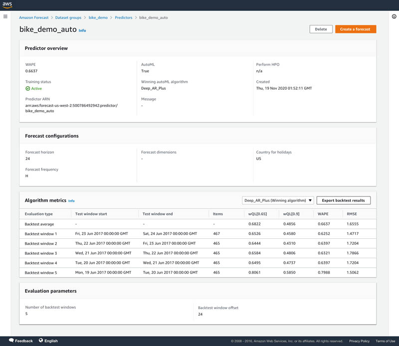
Forecast provides different model accuracy metrics for you to assess the strength of your forecasting models. We provide the weighted quantile loss (wQL) metric for each selected distribution point, and weighted absolute percentage error (WAPE) and root mean square error (RMSE), calculated at the mean forecast. For more information about how each metric is calculated and recommendations for the best use case for each metric, see Measuring forecast model accuracy to optimize your business objectives with Amazon Forecast.

Although Forecast provides these three industry-leading forecast accuracy measures, you might prefer to calculate accuracy using different metrics. With the launch of this feature, you can use the export of forecasts from backtesting to calculate the model accuracy using your own formula, without the need to generate forecasts and incur additional cost during experimentation.

After you experiment and finalize a forecasting model that works for you, you can continue to generate forecasts on a regular basis using the CreateForecast API.

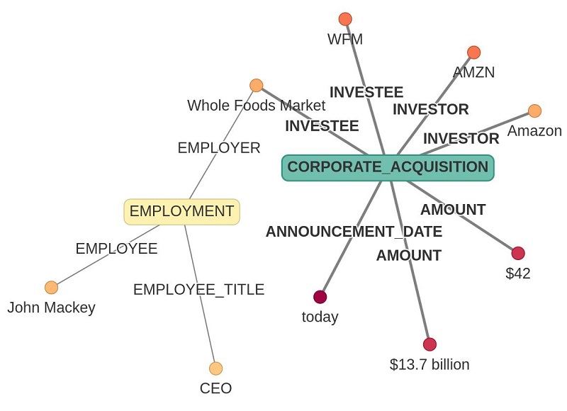
Exporting forecasts from backtesting and accuracy metrics for each item

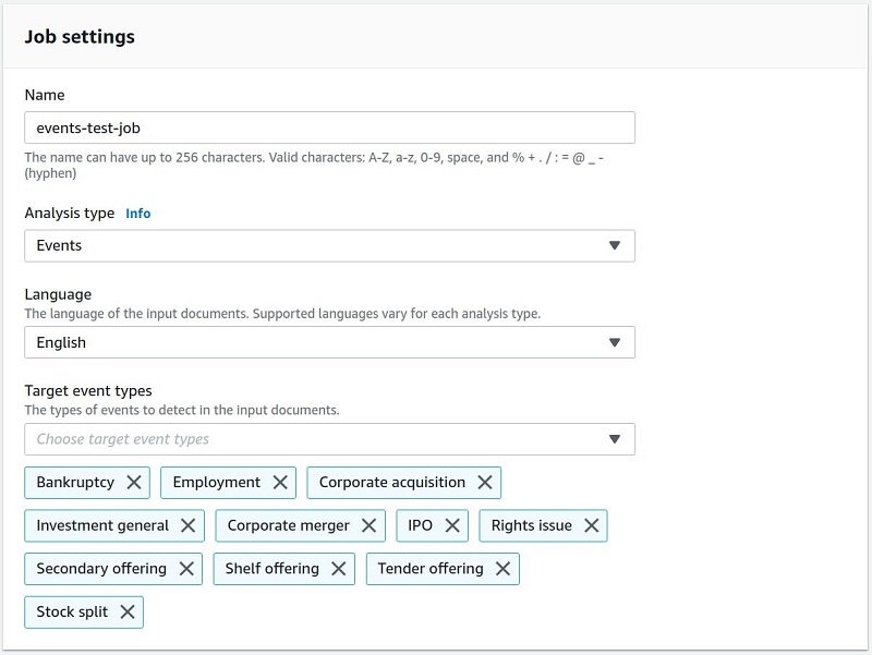
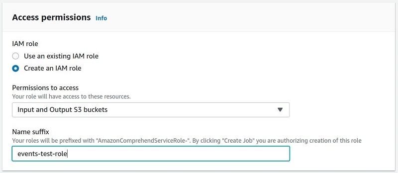
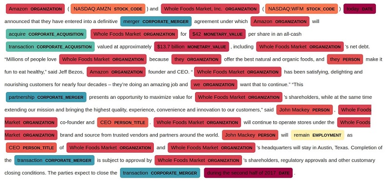
To use this new capability, use the newly launched CreatePredictorBacktestExportJob API after training a predictor. In this section, we walk through the steps on the Forecast console using the Bike Sharing dataset example in our GitHub repo. You can also refer to this notebook in our GitHub repo to follow through these steps using the Forecast APIs.

The bike sharing dataset forecasts the number of bike rides expected in a location. There are more than 400 locations in the dataset.

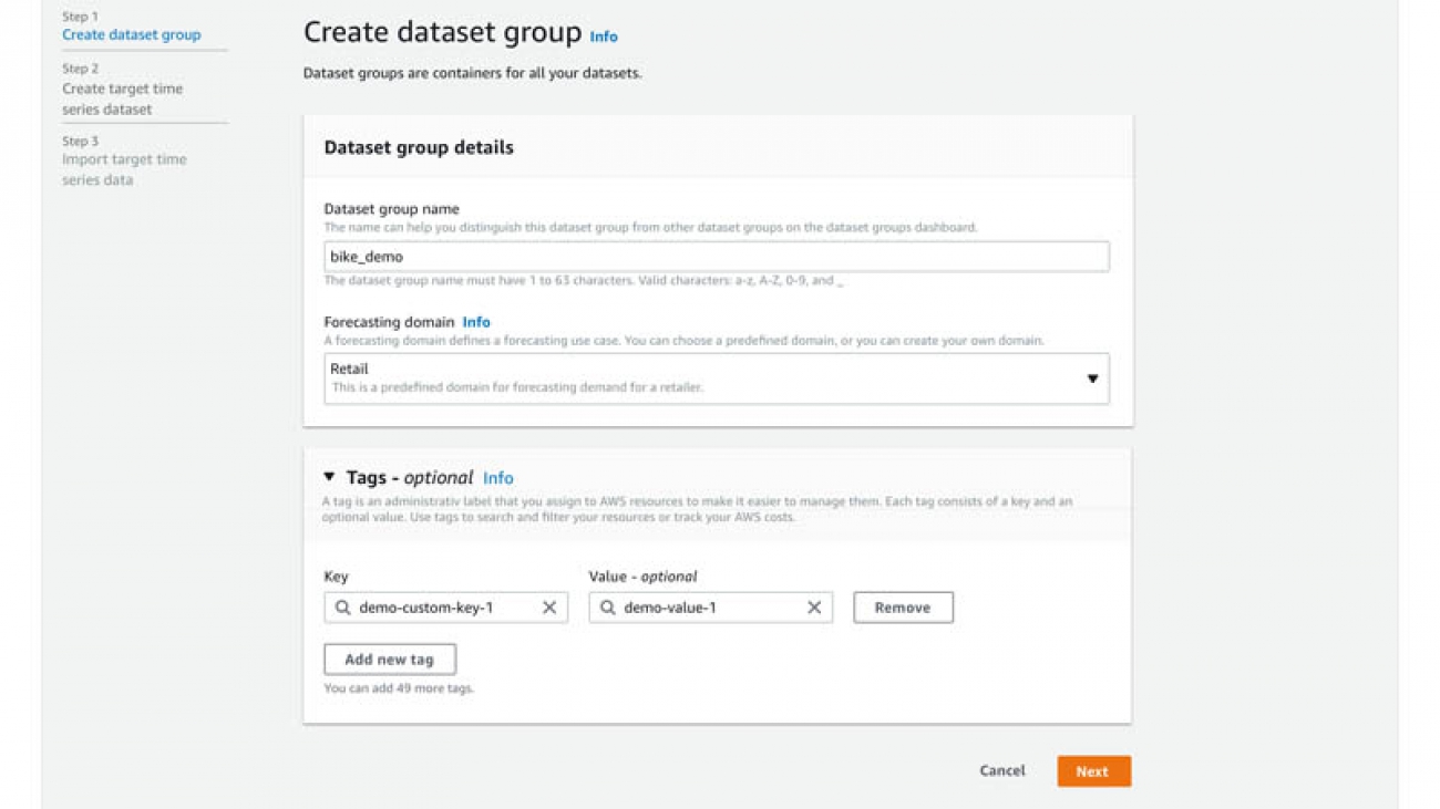
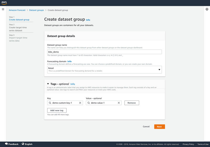
1. On the Forecast console, create a dataset group.

2. Upload the target time series file from the bike dataset.

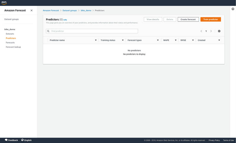
3. In the navigation pane, choose Predictors.
4. Choose Train predictor.

5. For training a predictor, we use the following configuration:

1. 1. For Forecast horizon, choose 24.
   2. For Forecast frequency, set to hourly.
   3. For Number of backtest windows, choose 5.
   4. For Backtest window offset, choose 24.
   5. For Forecast types, enter mean, 65, and 0.90.
   6. For Algorithm, select Automatic (AutoML).

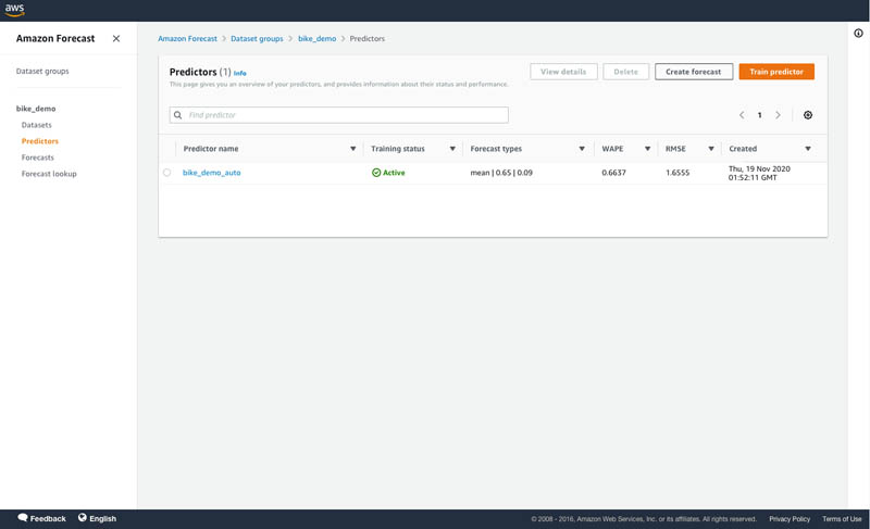
6. After your predictor is trained, choose your predictor on the Predictors page to view details of the accuracy metrics.

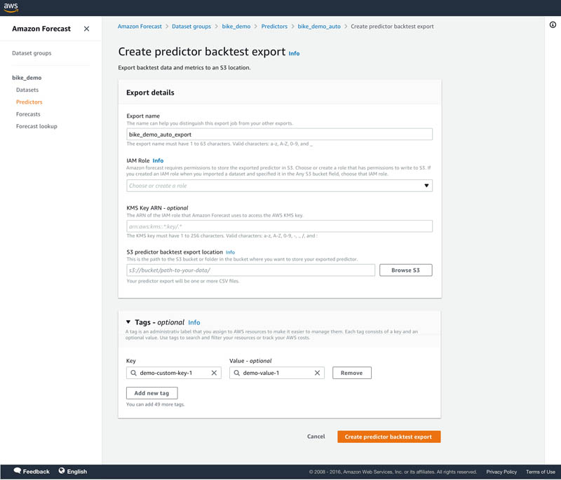
7. On the predictor’s details page, choose Export backtest results in the Predictor metrics

8. For S3 predictor backtest export location, enter the details of your Amazon Simple Storage Service (Amazon S3) location for exporting the CSV files.

Two type of files are exported to the Amazon S3 location in two different folders:

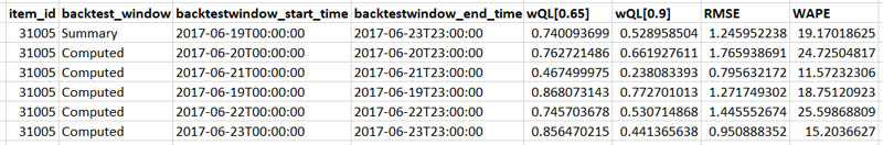
• forecasted-values – Contains the forecasts from each backtest window. The file name convention is Forecasts_PredictorBacktestExportJobName_CurrentTimestamp_PartNumber.csv. For this post, the file name is Forecasts_bike_demo_auto_export_2020-11-19-00Z_part0.csv.
• accuracy-metrics-values – Contains the accuracy metrics for each item per backtest window. The file name convention is Accuracy_ PredictorBacktestExportJobName_CurrentTimestamp_PartNumber.csv. For this post, the file name is Accuracy_bike_demo_auto_export_2020-11-19-00Z_part0.csv.

The wQL, WAPE, and RMSE metrics are provided for the accuracy metric file. Sometimes, output files are split into multiple parts based on the size of the output and are given numbering like part0, part1, and so on.

The following screenshot shows part of the Forecasts_bike_demo_auto_export_2020-11-19-00Z_part0.csv file from the bike dataset backtest exports.

The following screenshot shows part of the Accuracy_bike_demo_auto_export_2020-11-19-00Z_part0.csv file from the bike dataset backtest exports.

9. After you finalize your predictor, choose Forecasts in the navigation pane.
10. Choose Create a forecast.
11. Select your trained predictor to create a forecast.

Visualizing backtest forecasts and item accuracy metrics

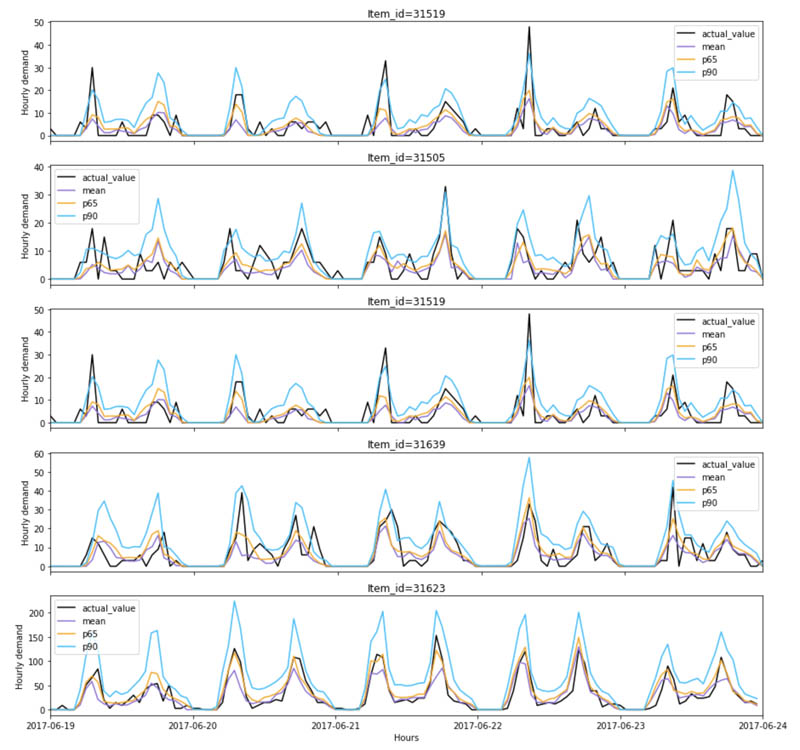
With the backtest forecasts, you can use a visualization tool like Amazon QuickSight to create graphs that help you visualize and compare the forecasts against actuals and graphically assess accuracy. In our notebook, we walk through some visualization examples for your reference. The graph below visualizes the backtest forecasts at different distributions points and the actual observed demand for different items.

Calculating custom metrics

We provide the following model accuracy metrics: weighted quantile loss (wQL) metric, weighted absolute percentage error (WAPE) and root mean square error (RMSE). Now with the export of the backtest forecasts, you can also calculate custom model accuracy metrics such as MAPE using the following formula:

In our notebook, we discuss how you can calculate MAPE and metrics for slow- and fast-moving items.

Tips and best practices

In this section, we share a few tips and best practices when using Forecast:

• Before experimenting with Forecast, define your business problem related to costs of under-forecasting or over-forecasting. Evaluate the trade-offs and prioritize if you would rather over-forecast than under. This helps you determine the forecasting quantile to choose.
• Experiment with multiple distribution points to optimize your forecast model to balance the costs associated with under-forecasting and over-forecasting. Choose a higher quantile if you want to over-forecast to meet demand. The backtest forecasts and accuracy metric files help you assess and optimize the model’s performance against under-forecasting and over-forecasting.
• If you’re comparing different models, use the weighted quantile loss metric at the same quantile for comparison. The lower the value, the more accurate the forecasting model.
• Forecast allows you to select up to five backtest windows. Forecast uses backtesting to tune predictors and produce accuracy metrics. To perform backtesting, Forecast automatically splits your time series datasets into two sets: training and testing. The training set is used to train your model, and the testing set to evaluate the model’s predictive accuracy. We recommend choosing more than one backtest window to minimize selection bias that may make one window more or less accurate by chance. Assessing the overall model accuracy from multiple backtest windows provides a better measure of the strength of the model.
• To create mean forecasts, specify mean as a forecast type. A forecast type of 0.5 refers to the median quantile.
• The wQL metric is not defined for the mean forecast type. However, the WAPE and RMSE metrics are calculated at mean. To view the wQL metric, specify a forecast type of 0.5.
• If you want to calculate a custom metric, such as MAPE, specify mean as a forecast type, and use the backtest forecasts corresponding to mean for this calculation.

Conclusion

Some items may be more important than others in a dataset, and optimizing accuracy for those important items becomes critical. Forecast now supports forecast accuracy measurement for each item separately, enabling you to make better forecasting decisions for items that drive your business metrics. To get started with this capability, see the CreatePredictorBacktestExportJob API. We also have a notebook in our GitHub repo that walks you through how to use the Forecast APIs to export accuracy measurements of each item and calculate accuracy metrics for a custom set of items. You can use this capability in all Regions where Forecast is publicly available. For more information about Region availability, see Region Table.

About the Authors

Namita Das is a Sr. Product Manager for Amazon Forecast. Her current focus is to democratize machine learning by building no-code/low-code ML services. On the side, she frequently advises startups and is raising a puppy named Imli.

 Punit Jain is working as SDE on the Amazon Forecast team. His current work includes building large scale distributed systems to solve complex machine learning problems with high availability and low latency as a major focus. In his spare time, he enjoys hiking and cycling.

Christy Bergman is working as an AI/ML Specialist Solutions Architect at AWS. Her work involves helping AWS customers be successful using AI/ML services to solve real world business problems. Prior to joining AWS, Christy worked as a Data Scientist in banking and software industries. In her spare time, she enjoys hiking and bird watching.

Read More

¡Amazon Lex lanza soporte para español para América Latina! Amazon Lex startet auf Deutsch!

Amazon Lex is a service for building conversational interfaces into any application using voice and text. Starting today, Amazon Lex supports Latin American Spanish and German. Now you can easily create virtual agents, conversational IVR systems, self-service chatbots, or application bots to answer and resolve questions for your Latin American Spanish and German speakers.

Customer stories

To increase employee productivity and provide a better customer service experience, companies are looking to create more ways for their customers to get their questions answered and tasks completed. See how some of our customers are using Amazon Lex to create virtual contact center agents, chat interfaces, and knowledge management bots.

Xpertal

Fomento Económico Mexicano, S.A.B. de C.V., or FEMSA, is a Mexican multinational beverage and retail company. Xpertal Global Services is FEMSA’s Service Unit, offering consulting, IT, back-office transactional, and consumable procurement services to the rest of FEMSA’s business units. One of Xpertal’s services operates an internal help desk comprised of 150-agent Contact Center that handles approximately 4 million calls per year.

As Xpertal shares in the post How Xpertal is creating the Contact Center of the future with Amazon Lex, they first started to build Amazon Lex bots with US Spanish for multiple internal web portals and integrated it with Amazon Connect to their Contact Center. With today’s launch of Latin American Spanish, they are excited to migrate and create an even more localized experience for their customers.

Xpertal’s Contact Center Manager, Chester Perez, shares, “Our goal is to keep evolving as an organization and find better ways to deliver our products and improve customer satisfaction. Our talented internal team developed various initiatives focused on bringing more intelligence and automation into our contact center to provide self-service capabilities, improve call deflection rates, reduce call wait times, and increase agent productivity. Amazon Lex is simple to use and the Contact Center team was already creating bots after just a 1-hour enablement session.

“Thanks to AWS AI services, we can finally focus on how to apply the technology for our users’ benefit and not on what’s behind it.”

Decadia

Amazon Lex is also opening opportunities for Decadia, a provider of company pension plans in Germany. Joerg Passmann, an Executive Director at Decadia, says, “Providing quality corporate pension plans is our passion, and the concerns of our pension members are close to our hearts at Decadia. We’d love to address them around the clock. Amazon Lex gives us the opportunity to process inquiries outside of our regular service hours and to be available with adequate assistance at any time. We look forward to exploring the diverse fields of application as part of a pilot phase.”

E.ON

E.ON is the largest energy company in Europe. Dr. Juan Bernabé-Moreno, Chief Data Officer, says, “The energy world is changing at an unprecedented speed, and E.ON is actively shaping it. Handling the ever-increasing complexity requires a new approach to how we organize and manage our knowledge to better understand our customers, our competitors, our regulatory and political environment, and also the emerging trends and the new players. For that, we created an AI-powered knowledge management engine called Sophia. With Amazon Lex, we want to bring Sophia closer to each and every employee in the company, so that our decisions are always taken considering all the facts and knowledge available… in other words, we want to make Sophia part of each and every conversation, and Lex capabilities are quite promising to humanize Sophia.”

How to get started

Start exploring how you can apply Amazon Lex to your business processes.  This post shows you how to Expand Amazon Lex conversational experiences with Spanish. To use the new Amazon Lex languages, simply choose the language when creating a new bot via the Amazon Lex console or SDK.

For more information, see the Amazon Lex Developer Guide.

Conclusion

Amazon Lex is a powerful service for building conversational interfaces into your applications. Try using it to help increase call deflect rates, increase first call resolution rates, and reduce call times in your contact center. Or add it to the front of your knowledge bases to help your employees and customers find the answers they need faster. See all the ways in which other customers are using Amazon Lex.

About the Author

Esther Lee is a Product Manager for AWS Language AI Services. She is passionate about the intersection of technology and education. Out of the office, Esther enjoys long walks along the beach, dinners with friends and friendly rounds of Mahjong.

Read More

This is a joint blog post with AWS Solutions Architects, Jorge Alfaro Hidalgo and Mauricio Zajbert, and Chester Perez, the Contact Center Manager at Xpertal. Fomento Económico Mexicano, S.A.B. de C.V. (FEMSA) is a Mexican multinational beverage and retail company headquartered in Monterrey, Mexico.

Fomento Económico Mexicano, S.A.B. de C.V., or FEMSA, is a Mexican multinational beverage and retail company headquartered in Monterrey, Mexico. Xpertal Global Services is FEMSA’s service unit that offers consulting, IT, back-office transactional, and consumable procurement services to the rest of FEMSA’s business units. Xpertal operates a Contact Center which serves as an internal help desk for employees and has 150 agents that handles 4 million calls per year. Their goal is to automate the majority calls by 2023 with a chatbot and only escalate complex queries requiring human intervention to live agents.

The contact center started this transformation 2 years ago with Robotic Process Automation (RPA) solutions and it has already been a big success. They’ve removed repetitive tasks such as password resets and doubled the number of requests serviced with the same number of agents.

This technology was helpful, but to achieve the next level of automation, they needed to start looking at systems that could naturally emulate human interactions. This is where Amazon AI has been helpful. As part of the journey, Xpertal started exploring Amazon Lex, a service to create self-service virtual agents to improve call response times. In addition, they used other AI services such as Amazon Comprehend, Amazon Polly, and Amazon Connect to automate other parts of the contact center.

In the first stage, Xpertal used Amazon Comprehend, a natural language processing service to classify support request emails automatically and route them to the proper resolution teams. This process used to take 4 hours to perform manually, and was reduced to 15 minutes with Amazon Comprehend.

Next, Xpertal started to build bots supporting US Spanish with Amazon Lex for multiple internal websites. They’ve been able to optimize each bot to fit each business units’ need and integrate it with Amazon Connect, an omni-channel cloud contact center. Then the Lex bot can also help to resolve employee calls coming into the Contact Center. With today’s launch of Latin American Spanish, they are excited to migrate and create an even more localized experience for their employees.

It was easy to integrate Amazon Lex with Amazon Connect and other third-party collaboration tools used within FEMSA to achieve an omni-channel system for support requests. Some of the implemented channels include email, phone, collaboration tools, and internal corporate websites.

In addition, Amazon Lex has been integrated with a diverse set of information sources within FEMSA to create a virtual help desk that enables their employees to find answers faster. These information sources include their CRM and internal ticketing systems. It’s now possible for users to easily chat with the help desk system to create support tickets or get a status update. They’ve also been able to build these types of conversational interactions with other systems and databases to provide more natural responses to users.

The following diagram shows the solution architecture for Xpertal’s Contact Center.

This architecture allows calls coming into the Contact Center to be routed to Amazon Connect. Amazon Connect then invokes Amazon Lex to identify the caller’s need. Subsequently, Amazon Lex uses AWS Lambda to interact with applications’ databases to either fulfill the user’s need by retrieving the information needed or creating a ticket to escalate the user’s request to the appropriate support team.

In addition, all customer calls are recorded and transcribed with Amazon Transcribe for post-call analytics to identify improvement areas and usage trends. The Xpertal team is effectively able to track user interactions. By analyzing the user utterances the bot didn’t understand, the team is able to monitor the solution’s effectiveness and continuously improve containment rates.

Xpertal’s Contact Center Manager, Chester Perez, shares, “Our goal is to keep evolving as an organization and find better ways to deliver our products and improve customer satisfaction. Our talented internal team developed various initiatives focused on bringing more intelligence and automation into our internal contact center to provide self-service capabilities, improve call deflection rates, reduce call wait times, and increase agent productivity. With Amazon Lex’s easy to use interface, our Contact Center team was able to create bots after a 1-hour training session. Thanks to AWS AI services, we can finally focus on how to apply the technology for our users’ benefit and not on what’s behind it.”

Summary

AWS has been working with a variety of customers such as Xpertal to find ways for AI services like Amazon Lex to boost self-service capabilities that lead to call containment and improve the overall contact center productivity and customer experience in Spanish.

Get started with this “How to create a virtual call center agent with Amazon Lex” tutorial with any of our localized Spanish language choices. Amazon Lex now offers Spanish, US Spanish, and LATAM Spanish. Depending on your contact center goals, learn more about Amazon Connect’s omni-channel, cloud-based contact center or bring your own telephony (BYOT) with AWS Contact Center Intelligence.

About the Authors

Chester Perez has 17 years working with FEMSA group, has contributed in areas of development, infrastructure and architecture. He has also designed and implemented teams that provide specialized support and center of excellence in data center. He is currently Manager of the Contact Center at Xpertal and his main challenge is to improve the quality and efficiency of the service it provides, by transforming the area into a technological and internal talent sense.

Jorge Alfaro Hidalgo is an Enterprise Solutions Architect in AWS Mexico with more than 20 years of experience in IT industry, he is passionate about helping enterprises to AWS cloud journey building innovative solutions to achieve their business objectives.

Mauricio Zajbert has more than 30 years of experience in the IT industry and a fully recovered infrastructure professional; he’s currently Solutions Architecture Manager for Enterprise accounts in AWS Mexico leading a team that helps customers in their cloud journey. He’s lived through several technology waves and deeply believes none has offered the benefits of the cloud.

Read More

Every day, financial organizations need to analyze news articles, SEC filings, and press releases, as well as track financial events such as bankruptcy announcements, changes in executive leadership at companies, and announcements of mergers and acquisitions. They want to accurately extract the key data points and associations among various people and organizations mentioned within an announcement to update their investment models in a timely manner. Traditional natural language processing services can extract entities such as people, organizations and locations from text, but financial analysts need more. They need to understand how these entities relate to each other in the text.

Today, Amazon Comprehend is launching Comprehend Events, a new API for event extraction from natural language text documents. With this launch, you can use Comprehend Events to extract granular details about real-world events and associated entities expressed in unstructured text. This new API allows you to answer who-what-when-where questions over large document sets, at scale and without prior NLP experience.

This post gives an overview of the NLP capabilities that Comprehend Events supports, along with suggestions for processing and analyzing documents with this feature. We’ll close with a discussion of several solutions that use Comprehend Events, such as knowledge base population, semantic search, and document triage, all of which can be developed with companion AWS services for storing, visualizing, and analyzing the predictions made by Comprehend Events.

Comprehend Events overview

The Comprehend Events API, under the hood, converts unstructured text into structured data that answers who-what-when-where-how questions. Comprehend Events lets you extract the event structure from a document, distilling pages of text down to easily processed data for consumption by your AI applications or graph visualization tools. In the following figure, an Amazon press release announcing the 2017 acquisition of Whole Foods Market, Inc. is rendered as a graph showing the core semantics of the acquisition event, as well as the status of Whole Foods’ CEO post merger.

Amazon (AMZN) today announced that they will acquire Whole Foods Market (WFM) for $42 per share in an all-cash transaction valued at approximately $13.7 billion, including Whole Foods Market’s net debt. Whole Foods Market will continue to operate stores under the Whole Foods Market brand and source from trusted vendors and partners around the world. John Mackey will remain as CEO of Whole Foods Market and Whole Foods Market’s headquarters will stay in Austin, Texas.

From: Amazon Press Center Release Archive

Extracted event triggers – Which events took place. In our example, CORPORATE_ACQUISITION and EMPLOYMENT events were detected. Not shown in the preceding figure, the API also returns which words in the text indicate the occurrence of the event, for example the words “acquire” and “transaction” in the context of the document indicate that a CORPORATE_ACQUISITION took place. The Comprehend Events API returns a variety of insights into the event semantics of a document:

• Extracted entity mentions – Which words in the text indicate which entities are involved in the event, including named entities such as “Whole Foods Market” and common nouns such as “today.” The API also returns the type of the entity detected, for example ORGANIZATION for “Whole Foods Market.”
• Event argument role (also known as slot filling) – Which entities play which roles in which events; for example Amazon is an INVESTOR in the acquisition event.
• Groups of coreferential event triggers – Which triggers in the document refer to the same event. The API also groups triggers such as “transaction” and “acquire” around the CORPORATE_ACQUISITION event (not shown above).
• Groups of coreferential entity mentions – Which mentions in the document refer to the same entity. For example, the API returns the grouping of “Amazon” with “they” as a single entity (not shown above).

At the time of launch, Comprehend Events is available as an asynchronous API supporting extraction of a fixed set of event types in the finance domain. This domain includes a variety of event types (such as CORPORATE_ACQUISITION and IPO), both standard and novel entity types (such as PER and ORG vs. STOCK_CODE and MONETARY_VALUE), and the argument roles that can connect them (such as INVESTOR, OFFERING_DATE, or EMPLOYER). For the complete ontology, see the Detect Events API documentation.

To demonstrate the functionality of the feature, we’ll show you how to process a small set of sample documents, using both the Amazon Comprehend console and the Python SDK.

Formatting documents for processing

The first step is to transform raw documents into a suitable format for processing. Comprehend Events imposes a few requirements on document size and composition:

• Individual documents must be UTF-8 encoded and no more than 10 KB in length. As a best practice, we recommend segmenting larger documents at logical boundaries (section headers) or performing sentence segmentation with existing open-source tools.
• For best performance, markup (such as HTML), tabular material, and other non-prose spans of text should be removed from documents. The service is intended to process paragraphs of unstructured text.
• A single job must not contain more than 50 MB of data. Larger datasets must be divided into smaller sets of documents for parallel processing. The different document format modes also impose size restrictions:
  • One document per file (ODPF) – A maximum of 5,000 files in a single Amazon Simple Storage Service (Amazon S3) location.
  • One document per line (ODPL) – A maximum of 5,000 lines in a single text file. Newline characters (n, r, rn) should be replaced with other whitespace characters within a given document.

For this post, we use a set of 117 documents sampled from Amazon’s Press Center: sample_finance_dataset.txt. The documents are formatted as a single ODPL text file and already conform to the preceding requirements. To implement this solution on your own, just upload the text file to an S3 bucket in your account before continuing with the following steps.

Job creation option 1: Using the Amazon Comprehend console

Creating a new Events labeling job takes only a few minutes.

1. On the Amazon Comprehend console, choose Analysis jobs.
2. Chose Create job.
3. For Name, enter a name (for this post, we use events-test-job).
4. For Analysis type¸ choose Events.
5. For Language, choose English.
6. For Target event types, choose your types of events (for example, Corporate acquisition).

7. In the Input data section, for S3 location, enter the location of the sample ODPL file you downloaded earlier.
8. In the Output data section, for S3 location, enter a location for the event output.

9. For IAM role, choose to use an existing AWS Identity and Access (IAM) role or create a new one.

10. Choose Create job. 

A new job appears in the Analysis jobs queue.

Job creation option 2: Using the SDK

Alternatively, you can perform these same steps with the Python SDK. First, we specify Comprehend Events job parameters, just as we would with any other Amazon Comprehend feature. See the following code:

# Client and session information
session = boto3.Session()
comprehend_client = session.client(service_name="comprehend")

# Constants for S3 bucket and input data file.
bucket = "comprehend-events-blogpost-us-east-1"
filename = 'sample_finance_dataset.txt'
input_data_s3_path = f's3://{bucket}/' + filename
output_data_s3_path = f's3://{bucket}/'

# IAM role with access to Comprehend and specified S3 buckets
job_data_access_role = 'arn:aws:iam::xxxxxxxxxxxxx:role/service-role/AmazonComprehendServiceRole-test-events-role'

# Other job parameters
input_data_format = 'ONE_DOC_PER_LINE'
job_uuid = uuid.uuid1()
job_name = f"events-job-{job_uuid}"
event_types = ["BANKRUPTCY", "EMPLOYMENT", "CORPORATE_ACQUISITION", 
               "INVESTMENT_GENERAL", "CORPORATE_MERGER", "IPO",
               "RIGHTS_ISSUE", "SECONDARY_OFFERING", "SHELF_OFFERING",
               "TENDER_OFFERING", "STOCK_SPLIT"]

Next, we use the start_events_detection_job API endpoint to start the analysis of the input data file and capture the job ID, which we use later to poll and retrieve results:

# Begin the inference job
response = comprehend_client.start_events_detection_job(
    InputDataConfig={'S3Uri': input_data_s3_path,
                     'InputFormat': input_data_format},
    OutputDataConfig={'S3Uri': output_data_s3_path},
    DataAccessRoleArn=job_data_access_role,
    JobName=job_name,
    LanguageCode='en',
    TargetEventTypes=event_types
)

# Get the job ID
events_job_id = response['JobId']

An asynchronous Comprehend Events job typically takes a few minutes for a small number of documents and up to several hours for lengthier inference tasks. For our sample dataset, inference should take approximately 20 minutes. It’s helpful to poll the API using the describe_events_detection_job endpoint. When the job is complete, the API returns a JobStatus of COMPLETED. See the following code:

# Get current job status
job = comprehend_client.describe_events_detection_job(JobId=events_job_id)

# Loop until job is completed
waited = 0
timeout_minutes = 30
while job['EventsDetectionJobProperties']['JobStatus'] != 'COMPLETED':
    sleep(60)
    waited += 60
    assert waited//60 < timeout_minutes, "Job timed out after %d seconds." % waited
    job = comprehend_client.describe_events_detection_job(JobId=events_job_id)

Finally, we collect the Events inference output from Amazon S3 and convert to a list of dictionaries, each of which contains the predictions for a given document:

# The output filename is the input filename + ".out"
output_data_s3_file = job['EventsDetectionJobProperties']['OutputDataConfig']['S3Uri'] + filename + '.out'

# Load the output into a result dictionary    # Get the files.
results = []
with smart_open.open(output_data_s3_file) as fi:
    results.extend([json.loads(line) for line in fi.readlines() if line])

The Comprehend Events API output schema

When complete, the output is written to Amazon S3 in JSON lines format, with each line encoding all the event extraction predictions for a single document. Our output schema includes the following information:

• Comprehend Events system output contains separate objects for entities and events, each organized into groups of coreferential objects.
• The API output includes the text, character offset, and type of each entity mention and trigger.
• Event argument roles are linked to entity groups by an EntityIndex.
• Confidence scores for classification tasks are given as Score. Confidence of entity and trigger group membership is given with GroupScore.
• Two additional fields, File and Line, are present as well, allowing you to track document provenance.

The following Comprehend Events API output schema represents entities as lists of mentions and events as lists of triggers and arguments:

{ 
    "Entities": [
        {
            "Mentions": [
                {
                    "BeginOffset": number,
                    "EndOffset": number,
                    "Score": number,
                    "GroupScore": number,
                    "Text": "string",
                    "Type": "string"
                }, ...
            ]
        }, ...
    ],
    "Events": [
        {
            "Type": "string",
            "Arguments": [
                {
                    "EntityIndex": number,
                    "Role": "string",
                    "Score": number
                }, ...
            ],
            "Triggers": [
                {
                    "BeginOffset": number,
                    "EndOffset": number,
                    "Score": number,
                    "Text": "string",
                    "GroupScore": number,
                    "Type": "string"
                }, ...
            ]
        }, ...
    ]
    "File": "string",
    "Line": "string
}

Analyzing Events output

The API output encodes all the semantic relationships necessary to immediately produce several useful visualizations of any given document. We walk through a few such depictions of the data in this section, referring you to the Amazon SageMaker Jupyter notebook accompanying this post for the working Python code necessary to produce them. We use the press release about Amazon’s acquisition of Whole Foods mentioned earlier in this post as an example.

Visualizing entity and trigger spans

As with any sequence labeling task, one of the simplest visualizations for Comprehend Events output is highlighting triggers and entity mentions, along with their respective tags. For this post, we use displaCy‘s ability to render custom tags. In the following visualization, we see some of the the usual range of entity types detected by NER systems (PERSON, ORGANIZATION), as well as finance-specific ones, such as STOCK_CODE and MONETARY_VALUE. Comprehend Events detects non-named entities (common nouns and pronouns) as well as named ones. In addition to entities, we also see tagged event triggers, such as “merger” (CORPORATE_MERGER) and “acquire” (CORPORATE_ACQUISITION).

Graphing event structures

Highlighting tagged spans is informative because it localizes system predictions about entity and event types in the text. However, it doesn’t show the most informative thing about the output: the predicted argument role associations among events and entities. The following plot depicts the event structure of the document as a semantic graph. In the graph, vertices are entity mentions and triggers; edges are the argument roles held by the entities in relation to the triggers. For simple renderings of a small number of events, we recommend common open-source tools such as networkx and pyvis, which we used to produce this visualization. For larger graphs, and graphs of large numbers of documents, we recommend a more robust solution for graph storage, such as Amazon Neptune.

Tabulating event structures

Lastly, you can always render the event structure produced by the API as a flat table, indicating, for example, the argument roles of the various participants in each event, as in the following table. The table demonstrates how Comprehend Events groups entity mentions and triggers into coreferential groups. You can use these textual mention groups to verify and analyze system predictions.

Setting up the Comprehend Events AWS CloudFormation stack

You can quickly try out this example for yourself by deploying our sample code into your own account from the provided AWS CloudFormation template. We’ve included all the necessary steps in a Jupyter notebook, so you can easily walk through creating the preceding visualizations and see how it all works. From there, you can easily modify it to run over other custom datasets, modify the results, ingest them into other systems, and build upon the solution. Complete the following steps:

1. Choose Launch Stack:

2. After the template loads in the AWS CloudFormation console, choose Next.
3. For Stack name, enter a name for your deployment.
4. Choose Next.

5. Choose Next on the following page.
6. Select the check box acknowledging this template will create IAM resources.

This allows the SageMaker notebook instance to talk with Amazon S3 and Amazon Comprehend.

7. Choose Create stack.

8. When stack creation is complete, browse to your notebook instances on the SageMaker console.

A new instance is already loaded with the example data and Jupyter notebook.

9. Choose Open Jupyter for the comprehend-events-blog notebook.

The data and notebook are already loaded on the instance. This was done through a SageMaker lifecycle configuration.

10. Choose the notebooks folder.
11. Choose the comprehend_events_finance_tutorial.ipynb notebook.

12. Step through the notebook to try Comprehend Events out yourself.

Applications using Comprehend Events

We have demonstrated applying Comprehend Events to a small set of documents and demonstrated visualizing the event structures found in a sample document. The power of Comprehend Events, however, lies in its ability to extract and structure business-relevant facts from large collections of unstructured documents. In this section, we discuss a few potential solutions that you could build on top of the foundation provided by Comprehend Events.

Knowledge graph construction

Business and financial services analysts need to visually explore event-based relationships among corporate entities, identifying potential patterns over large collections of data. Without a tool like Comprehend Events, you have to manually identify entities of interests and events in documents and manually enter them in network visualization tools for tracking. Comprehend Events allows you to populate knowledge graphs over large collections of data. You can store these graphs and search, for example, in Neptune and explore using network visualization tools without expensive manual extraction.

Semantic search

Analysts also need to find documents in which actors of interest participate in events of interest (at places, at times). The most common approach to this task involves enterprise search: using complex Boolean queries to find co-occurring strings that typically match your desired search patterns. Natural language is rich and highly variable, however, and even the best searches often miss key details in unstructured text. Comprehend Events allows you to populate a search index with event-argument associations, enriching free text search with extracted event data. You can process collections of documents with Comprehend Events, index the documents in Amazon Elasticsearch Service (Amazon ES) with the extracted event data, and enable field-based search over event-argument tuples in downstream applications.

Document triage

An additional application of Comprehend Events is simple filtration of large text collections for events of interest. This task is typically performed with a tool such as Amazon Comprehend customer classification, but requires hundreds or thousands of annotated training documents to produce a custom model. Comprehend Events allows developers without such training data to process a large collection of documents and detect financial events found in the event taxonomy. You can simply process batches of documents with the asynchronous API and route documents matching pre-defined event patterns to downstream applications.

Conclusion

This post has demonstrated the application and utility of Comprehend Events for information processing in the finance domain. This new feature gives you the ability to enrich your applications with close semantic analysis of financial events from unstructured text, all without any NLP model training or tuning. For more information, just check out our documentation or try out the above walkthrough for yourself in the Console or in our Jupyter notebook through CloudFormation or on Github. We’re exciting to hear your comments and questions in the comments section!

About the Authors

Graham Horwood is a data scientist at Amazon AI. His work focuses on natural language processing technologies for customers in the public and commercial sectors.

Ben Snively is an AWS Public Sector Specialist Solutions Architect. He works with government, non-profit, and education customers on big data/analytical and AI/ML projects, helping them build solutions using AWS.

Sameer Karnik is a Sr. Product Manager leading product for Amazon Comprehend, AWS’s natural language processing service.

Read More

Amazon SageMaker Studio is the first fully integrated development environment (IDE) for machine learning (ML). With a single click, data scientists and developers can quickly spin up SageMaker Studio notebooks to explore datasets and build models. On October 27, 2020, Amazon released a custom images feature that allows you to launch SageMaker Studio notebooks with your own images.

SageMaker Studio notebooks provide a set of built-in images for popular data science and ML frameworks and compute options to run notebooks. The built-in SageMaker images contain the Amazon SageMaker Python SDK and the latest version of the backend runtime process, also called kernel. With the custom images feature, you can register custom built images and kernels, and make them available to all users sharing a SageMaker Studio domain. You can start by cloning and extending one of the example Docker files provided by SageMaker, or build your own images from scratch.

This post focuses on adding a custom R image to SageMaker Studio so you can build and train your R models with SageMaker. After attaching the custom R image, you can select the image in Studio and use R to access the SDKs using the RStudio reticulate package. For more information about R on SageMaker, see Coding with R on Amazon SageMaker notebook instances and R User Guide to Amazon SageMaker.

You can create images and image versions and attach image versions to your domain using the SageMaker Studio Control Panel, the AWS SDK for Python (Boto3), and the AWS Command Line Interface (AWS CLI)—for more information about CLI commands, see AWS CLI Command Reference. This post explains both AWS CLI and SageMaker console UI methods to attach and detach images to a SageMaker Studio domain.

Prerequisites

Before getting started, you need to meet the following prerequisites:

• Install the AWS CLI on your local machine. This post uses AWS CLI version 2. You should make necessary adjustments if you use a different AWS CLI version.
• Permissions to access the Amazon Elastic Container Registry (Amazon ECR). For more information, see Amazon ECR Managed Policies.
• Install Docker on your local machine. For more information, see Orientation and setup. This is necessary for building Docker images and pushing them to Amazon ECR.
  • For instructions on building a container from a Studio development environment, see Using the Amazon SageMaker Studio Image Build CLI to build container images from your Studio notebooks and the SageMaker Docker Build GitHub repo.
• Dockerfile for the R image. A sample Dockerfile is provided in this post that you can customize for your own specific case, but you can also use your own Dockerfile.
  • Building the R image from the Dockerfile installs dependencies that may be licensed under copyleft licenses such as GPLv3. You should review the license terms and make sure they are acceptable for your use case before proceeding to build this image.
• An AWS Identity and Access Management (IAM) role that has the AmazonSageMakerFullAccess policy attached. If you have onboarded to SageMaker Studio, you can get the role from the Studio Summary section on the SageMaker Studio Control Panel.
• A SageMaker Studio domain. For instructions, see Onboard to Amazon SageMaker Studio.

Creating your Dockerfile

Before attaching your image to Studio, you need to build a Docker image using a Dockerfile. You can build a customized Dockerfile using base images or other Docker image repositories, such as Jupyter Docker-stacks repository, and use or revise the ones that fit your specific need.

SageMaker maintains a repository of sample Docker images that you can use for common use cases (including R, Julia, Scala, and TensorFlow). This repository contains examples of Docker images that are valid custom images for Jupyter KernelGateway Apps in SageMaker Studio. These custom images enable you to bring your own packages, files, and kernels for use within SageMaker Studio.

For more information about the specifications that apply to the container image that is represented by a SageMaker image version, see Custom SageMaker image specifications.

For this post, we use the sample R Dockerfile. This Dockerfile takes the base Python 3.6 image and installs R system library prerequisites, conda via Miniconda, and R packages and Python packages that are usable via reticulate. You can create a file named Dockerfile using the following script and copy it to your installation folder. You can customize this Dockerfile for your specific use case and install additional packages.

# This project is licensed under the terms of the Modified BSD License 
# (also known as New or Revised or 3-Clause BSD), as follows:

#    Copyright (c) 2001-2015, IPython Development Team
#    Copyright (c) 2015-, Jupyter Development Team

# All rights reserved.

FROM python:3.6

ARG NB_USER="sagemaker-user"
ARG NB_UID="1000"
ARG NB_GID="100"

# Setup the "sagemaker-user" user with root privileges.
RUN 
    apt-get update && 
    apt-get install -y sudo && 
    useradd -m -s /bin/bash -N -u $NB_UID $NB_USER && 
    chmod g+w /etc/passwd && 
    echo "${NB_USER}    ALL=(ALL)    NOPASSWD:    ALL" >> /etc/sudoers && 
    # Prevent apt-get cache from being persisted to this layer.
    rm -rf /var/lib/apt/lists/*

USER $NB_UID

# Make the default shell bash (vs "sh") for a better Jupyter terminal UX
ENV SHELL=/bin/bash 
    NB_USER=$NB_USER 
    NB_UID=$NB_UID 
    NB_GID=$NB_GID 
    HOME=/home/$NB_USER 
    MINICONDA_VERSION=4.6.14 
    CONDA_VERSION=4.6.14 
    MINICONDA_MD5=718259965f234088d785cad1fbd7de03 
    CONDA_DIR=/opt/conda 
    PATH=$CONDA_DIR/bin:${PATH}

# Heavily inspired from https://github.com/jupyter/docker-stacks/blob/master/r-notebook/Dockerfile

USER root

# R system library pre-requisites
RUN apt-get update && 
    apt-get install -y --no-install-recommends 
    fonts-dejavu 
    unixodbc 
    unixodbc-dev 
    r-cran-rodbc 
    gfortran 
    gcc && 
    rm -rf /var/lib/apt/lists/* && 
    mkdir -p $CONDA_DIR && 
    chown -R $NB_USER:$NB_GID $CONDA_DIR && 
    # Fix for devtools https://github.com/conda-forge/r-devtools-feedstock/issues/4
    ln -s /bin/tar /bin/gtar

USER $NB_UID

ENV PATH=$CONDA_DIR/bin:${PATH}

# Install conda via Miniconda
RUN cd /tmp && 
    curl --silent --show-error --output miniconda-installer.sh https://repo.anaconda.com/miniconda/Miniconda3-${MINICONDA_VERSION}-Linux-x86_64.sh && 
    echo "${MINICONDA_MD5} *miniconda-installer.sh" | md5sum -c - && 
    /bin/bash miniconda-installer.sh -f -b -p $CONDA_DIR && 
    rm miniconda-installer.sh && 
    conda config --system --prepend channels conda-forge && 
    conda config --system --set auto_update_conda false && 
    conda config --system --set show_channel_urls true && 
    conda install --quiet --yes conda="${CONDA_VERSION%.*}.*" && 
    conda update --all --quiet --yes && 
    conda clean --all -f -y && 
    rm -rf /home/$NB_USER/.cache/yarn


# R packages and Python packages that are usable via "reticulate".
RUN conda install --quiet --yes 
    'r-base=4.0.0' 
    'r-caret=6.*' 
    'r-crayon=1.3*' 
    'r-devtools=2.3*' 
    'r-forecast=8.12*' 
    'r-hexbin=1.28*' 
    'r-htmltools=0.4*' 
    'r-htmlwidgets=1.5*' 
    'r-irkernel=1.1*' 
    'r-rmarkdown=2.2*' 
    'r-rodbc=1.3*' 
    'r-rsqlite=2.2*' 
    'r-shiny=1.4*' 
    'r-tidyverse=1.3*' 
    'unixodbc=2.3.*' 
    'r-tidymodels=0.1*' 
    'r-reticulate=1.*' 
    && 
    pip install --quiet --no-cache-dir 
    'boto3>1.0<2.0' 
    'sagemaker>2.0<3.0' && 
    conda clean --all -f -y

WORKDIR $HOME
USER $NB_UID

Setting up your installation folder

You need to create a folder on your local machine and add the following files in that folder:

.
├── Dockerfile
├── app-image-config-input.json
├── create-and-attach-image.sh
├── create-domain-input.json
└── default-user-settings.json

In the following scripts, the Amazon Resource Names (ARNs) should have a format similar to:

arn:partition:service:region:account-id:resource-id
arn:partition:service:region:account-id:resource-type/resource-id
arn:partition:service:region:account-id:resource-type:resource-id

1. Dockerfile is the Dockerfile that you created in the previous step.

2. Create a file named app-image-config-input.json with the following content:

   {
       "AppImageConfigName": "custom-r-image-config",
       "KernelGatewayImageConfig": {
           "KernelSpecs": [
               {
                   "Name": "ir",
                   "DisplayName": "R (Custom R Image)"
               }
           ],
           "FileSystemConfig": {
               "MountPath": "/home/sagemaker-user",
               "DefaultUid": 1000,
               "DefaultGid": 100
           }
       }

3. Create a file named default-user-settings.json with the following content. If you’re adding multiple custom images, add to the list of CustomImages.

   {
     "DefaultUserSettings": {
       "KernelGatewayAppSettings": {
         "CustomImages": [
             {
                      "ImageName": "custom-r",
                      "AppImageConfigName": "custom-r-image-config"
                   }
               ]
           }
       }
   }

4. Create one last file in your installation folder named create-and-attach-image.sh using the following bash script. The script runs the following in order:
   1. Creates a repository named smstudio-custom in Amazon ECR and logs into that repository
   2. Builds an image using the Dockerfile and attaches a tag to the image r
   3. Pushes the image to Amazon ECR
   4. Creates an image for SageMaker Studio and attaches the Amazon ECR image to that image
   5. Creates an AppImageConfigfor this image using app-image-config-input.json

      # Replace with your AWS account ID and your Region, e.g. us-east-1, us-west-2
      ACCOUNT_ID = <AWS ACCOUNT ID>
      REGION = <STUDIO DOMAIN REGION>
      
      # create a repository in ECR, and then login to ECR repository
      aws --region ${REGION} ecr create-repository --repository-name smstudio-custom
      aws ecr --region ${REGION} get-login-password | docker login --username AWS 
          --password-stdin ${ACCOUNT_ID}.dkr.ecr.${REGION}.amazonaws.com/smstudio-custom
      
      # Build the docker image and push to Amazon ECR (modify image tags and name as required)
      $(aws ecr get-login --region ${REGION} --no-include-email)
      docker build . -t smstudio-r -t ${ACCOUNT_ID}.dkr.ecr.${REGION}.amazonaws.com/smstudio-custom:r
      docker push ${ACCOUNT_ID}.dkr.ecr.${REGION}.amazonaws.com/smstudio-custom:r
      
      # Using with SageMaker Studio
      ## Create SageMaker Image with the image in ECR (modify image name as required)
      ROLE_ARN = "<YOUR EXECUTION ROLE ARN>"
      
      aws sagemaker create-image 
          --region ${REGION} 
          --image-name custom-r 
          --role-arn ${ROLE_ARN}
      
      aws sagemaker create-image-version 
          --region ${REGION} 
          --image-name custom-r 
          --base-image ${ACCOUNT_ID}.dkr.ecr.${REGION}.amazonaws.com/smstudio-custom:r
      
      ## Create AppImageConfig for this image (modify AppImageConfigName and 
      ## KernelSpecs in app-image-config-input.json as needed)
      ## note that 'file://' is required in the file path
      aws sagemaker create-app-image-config 
          --region ${REGION} 
          --cli-input-json file://app-image-config-input.json

Updating an existing SageMaker Studio domain with a custom image

If you already have a Studio domain, you don’t need to create a new domain, and can easily update your existing domain by attaching the custom image. You can do this either using the AWS CLI for Amazon SageMaker or the SageMaker Studio Control Panel (which we discuss in the following sections). Before going to the next steps, make sure your domain is in Ready status, and get your Studio domain ID from the Studio Control Panel. The domain ID should be in d-xxxxxxxx format.

Using the AWS CLI for SageMaker

In the terminal, navigate to your installation folder and run the following commands. This makes the bash scrip executable:

chmod +x create-and-attach-image.sh

Then execute the following command in terminal:

./create-and-attach-image.sh

After you successfully run the bash script, you need update your existing domain by executing the following command in the terminal. Make sure you provide your domain ID and Region.

aws sagemaker update-domain --domain-id <DOMAIN_ID> 
    --region <REGION_ID> 
    --cli-input-json file://default-user-settings.json

After executing this command, your domain status shows as Updating for a few seconds and then shows as Ready again. You can now open Studio.

When in the Studio environment, you can use the Launcher to launch a new activity, and should see the custom-r (latest) image listed in the dropdown menu under Select a SageMaker image to launch your activity.

Using the SageMaker console

Alternatively, you can update your domain by attaching the image via the SageMaker console. The image that you created is listed on the Images page on the console.

1. To attach this image to your domain, on the SageMaker Studio Control Panel, under Custom images attached to domain, choose Attach image.
2. For Image source, choose Existing image.
3. Choose an existing image from the list.
4. Choose a version of the image from the list.
5. Choose Next.
6. Choose the IAM role. For more information, see Create a custom SageMaker image (Console).
7. Choose Next.
8. Under Studio configuration, enter or change the following settings. For information about getting the kernel information from the image, see DEVELOPMENT in the SageMaker Studio Custom Image Samples GitHub repo.
   1. For EFS mount path, enter the path within the image to mount the user’s Amazon Elastic File System (Amazon EFS) home directory.
   2. For Kernel name, enter the name of an existing kernel in the image.
   3. (Optional) For Kernel display name, enter the display name for the kernel.
   4. Choose Add kernel.
   5. (Optional) For Configuration tags, choose Add new tag and add a configuration tag.

For more information, see the Kernel discovery and User data sections of Custom SageMaker image specifications.

9. Choose Submit.
10. Wait for the image version to be attached to the domain.

While attaching, your domain status is in Updating. When attached, the version is displayed in the Custom images list and briefly highlighted, and your domain status shows as Ready.

The SageMaker image store automatically versions your images. You can select a pre-attached image and choose Detach to detach the image and all versions, or choose Attach image to attach a new version. There is no limit to the number of versions per image or the ability to detach images.

Using a custom image to create notebooks

When you’re done updating your Studio domain with the custom image, you can use that image to create new notebooks. To do so, choose your custom image from the list of images in the Launcher. In this example, we use custom-r. This shows the list of kernels that you can use to create notebooks. Create a new notebook with the R kernel.

If this is the first time you’re using this kernel to create a notebook, it may take about a minute to start the kernel, and the Kernel Starting message appears on the lower left corner of your Studio. You can write R scripts while the kernel is starting but can only run your script after your kernel is ready. The notebook is created with a default ml.t3.medium instance attached to it. You can see R (Custom R Image) kernel and the instance type on the upper right corner of the notebook. You can change ML instances on the fly in SageMaker Studio. You can also right-size your instances for different workloads. For more information, see Right-sizing resources and avoiding unnecessary costs in Amazon SageMaker.

To test the kernel, enter the following sample R script in the first cell and run the script. This script tests multiple aspects, including importing libraries, creating a SageMaker session, getting the IAM role, and importing data from public repositories.

The abalone dataset in this post is from Dua, D. and Graff, C. (2019). UCI Machine Learning Repository [http://archive.ics.uci.edu/ml]. Irvine, CA: University of California, School of Information and Computer Science (http://archive.ics.uci.edu/ml/datasets/Abalone).

# Simple script to test R Kernel in SageMaker Studio

# Import reticulate, readr and sagemaker libraries
library(reticulate)
library(readr)
sagemaker <- import('sagemaker')

# Create a sagemaker session
session <- sagemaker$Session()

# Get execution role
role_arn <- sagemaker$get_execution_role()

# Read a csv file from UCI public repository
# Dua, D. and Graff, C. (2019). UCI Machine Learning Repository [http://archive.ics.uci.edu/ml]. 
# Irvine, CA: University of California, School of Information and Computer Science
data_file <- 'http://archive.ics.uci.edu/ml/machine-learning-databases/abalone/abalone.data'

# Copy data to a dataframe, rename columns, and show dataframe head
abalone <- read_csv(file = data_file, col_names = FALSE, col_types = cols())
names(abalone) <- c('sex', 'length', 'diameter', 'height', 'whole_weight', 'shucked_weight', 'viscera_weight', 'shell_weight', 'rings')
head(abalone)

If the image is set up properly and the kernel is running, the output should look like the following screenshot.

Listing, detaching, and deleting custom images

If you want to see the list of custom images attached to your Studio, you can either use the AWS CLI or go to SageMaker console to view the attached image in the Studio Control Panel.

Using the AWS CLI for SageMaker

To view your list of custom images via the AWS CLI, enter the following command in the terminal (provide the Region in which you created your domain):

aws sagemaker list-images --region <region-id> 

The response includes the details for the attached custom images:

{
    "Images": [
        {
            "CreationTime": "xxxxxxxxxxxx",
            "ImageArn": "arn:aws:sagemaker:us-east-2:XXXXXXX:image/custom-r",
            "ImageName": "custom-r",
            "ImageStatus": "CREATED",
            "LastModifiedTime": "xxxxxxxxxxxxxx"
        },
        ....
    ]
}

If you want to detach or delete an attached image, you can do it on the SageMaker Studio Control Panel (see Detach a custom SageMaker image). Alternatively, use the custom image name from your default-user-settings.json file and rerun the following command to update the domain by detaching the image:

aws sagemaker update-domain --domain-id <YOUR DOMAIN ID> 
    --cli-input-json file://default-user-settings.json

Then, delete the app image config:

aws sagemaker delete-app-image-config 
    --app-image-config-name custom-r-image-config

Delete the SageMaker image, which also deletes all image versions. The container images in Amazon ECR that are represented by the image versions are not deleted.

aws sagemaker delete-image 
    --region <region-id> 
    --image-name custom-r

After deleting the image, it will not be listed under custom images in SageMaker Studio. For more information, see Clean up resources.

Using the SageMaker console

You can also detach (and delete) images from your domain via the Studio Control Panel UI. To do so, under Custom images attached to domain, select the image and choose Detach. You have the option to also delete all versions of the image from your domain. This detaches the image from the domain.

Getting logs in Amazon CloudWatch

You can also get access to SageMaker Studio logs in Amazon CloudWatch, which you can use for troubleshooting your environment. The metrics are captured under the /aws/sagemaker/studio namespace.

To access the logs, on the CloudWatch console, choose CloudWatch Logs. On the Log groups page, enter the namespace to see logs associated with the Jupyter server and the kernel gateway.

For more information, see Log Amazon SageMaker Events with Amazon CloudWatch.

Conclusion

This post outlined the process of attaching a custom Docker image to your Studio domain to extend Studio’s built-in images. We discussed how you can update an existing domain with a custom image using either the AWS CLI for SageMaker or the SageMaker console. We also explained how you can use the custom image to create notebooks with custom kernels.

For more information, see the following resources:

• Bringing your own custom container image to Amazon SageMaker Studio notebooks
• R User Guide to Amazon SageMaker
• Coding with R on Amazon SageMaker notebook instances
• Amazon SageMaker Examples GitHub repo

About the Authors

Nick Minaie is an Artificial Intelligence and Machine Learning (AI/ML) Specialist Solution Architect, helping customers on their journey to well-architected machine learning solutions at scale. In his spare time, Nick enjoys family time, abstract painting, and exploring nature.

Sam Liu is a product manager at Amazon Web Services (AWS). His current focus is the infrastructure and tooling of machine learning and artificial intelligence. Beyond that, he has 10 years of experience building machine learning applications in various industries. In his spare time, he enjoys making short videos for technical education or animal protection.

Read More

Understanding the direction and context of an ever-evolving conversation is beneficial to building natural, human-like conversational interfaces. Being able to classify utterances as the conversation develops requires managing context across multiple turns. Consider a caller who asks their financial planner for insights regarding their monthly expenses: “What were my expenses this year?” They may also ask for more granular information, such as “How about for last month?” As the conversation progresses, the bot needs to understand if the context is changing and adjust its responses accordingly.

Amazon Lex is a service for building conversational interface in voice and text. Previously, you had to write code to manage context via session attributes. Depending on the intent, the code had to orchestrate the invocation of the next intent. As the conversation complexity and the intent count increased, managing the orchestration could become more cumbersome.

Starting today, Amazon Lex supports context management natively, so you can manage the context directly without the need for custom code. As initial prerequisite intents are filled, you can create contexts to invoke related intents. This simplifies bot design and expedites the creation of conversational experiences.

Use case

This post uses the following conversation to model a bot for financial planning:

User:    What was my income in August?
Agent:  Your income in August was $2345.
User:    Ok. How about September?
Agent:  Your income in September was $4567.
User:    What were my expenses in July?
Agent:  Your expenses for July were $123.
User:    Ok thanks. 

Building the Amazon Lex bot FinancialPlanner

In this post, we build an Amazon Lex bot called FinancialPlanner, which is available for download. Complete the following steps:

1. Create the following intents:
   1. ExpensesIntent – Elicits information, such as account ID and period, and provides expenses detail
   2. IncomeIntent – Elicits information, such as account ID and period, and provides income detail
   3. ExpensesFollowup – Invoked after expenses intent to respond to a follow-up query, such as “How about [expenses] last month?”
   4. IncomeFollowup – Invoked after income intent to respond to a follow-up query about income, such as “How about [income] last month?”
   5. Fallback – Captures any input that the bot can’t process by the configured intents

2. Set up context tags for the expenses intents.

The context management feature defines input tags and output tags that the bot developer can set. You use these tags to manage the conversation flow. For our use case, we set expenses as the output context tag in ExpensesIntent. We also use this as the input context for ExpensesFollowupIntent. We can also configure the output tag with a timeout, measured by conversation turns or seconds since the initial intent was invoked.

The following screenshot shows the Context configuration section on the Amazon Lex console.

The following screenshot shows the specific parameters for the expenses tag.

3. Set up context tags for the income intents.

Similar to expenses, we now set the context for income intents. For IncomeIntent, set the output context tag as income. We use this context as the input context for IncomeFollowupIntent.

4. Build the bot and test it on the Amazon Lex console.

To test the bot, provide the input “What were my expenses this year” followed by “How about last month?” For the second request, the bot selects ExpensesFollowupIntent because the expenses context is active. Alternatively, if you start with “What was my income this year?” followed by “How about last year?”, the bot invokes the IncomeFollowupIntent because the income context is active.

The following screenshot illustrates how the context tags are used to invoke the appropriate intent.

You can configure the behavior of the context attributes by editing the threshold. Editing the number of turns sets the limit for the number of interactions with the bot, and the number of seconds is from the original input tag being set. As long as the intent with the output tag occurs before the turn- or time-based timeout, the user can invoke the intent based on the input context.

Along with the context management feature, you can also set default slot values. You can set the slots to populate from a context, a session attribute, or a value. In our sample bot model, the {month} slot in ExpensesIntent is set to August as the default slot value.

Conclusion

With the new Amazon Lex context management feature, you can easily orchestrate when to enable intents based on prior intents, and pass specific user data values from one intent to another. This capability allows you to create sophisticated, multi-turn conversational experiences without having to write custom code. Context carry-over, along with default slot values, simplifies bot development and allows you to easily create more natural, conversational user experiences. For more information, see Setting Intent Context documentation.

About the Authors

Blake DeLee is a Rochester, NY-based conversational AI consultant with AWS Professional Services. He has spent five years in the field of conversational AI and voice, and has experience bringing innovative solutions to dozens of Fortune 500 businesses. Blake draws on a wide-ranging career in different fields to build exceptional chatbot and voice solutions.

As a Product Manager on the Amazon Lex team, Harshal Pimpalkhute spends his time trying to get machines to engage (nicely) with humans.

Esther Lee is a Product Manager for AWS Language AI Services. She is passionate about the intersection of technology and education. Out of the office, Esther enjoys long walks along the beach, dinners with friends and friendly rounds of Mahjong.

Read More

When translating the English phrase “How are you?” to Spanish, would you prefer to use “¿Cómo estás?” or “¿Cómo está usted?” instead?

Amazon Translate is a neural machine translation service that delivers fast, high-quality, and affordable language translation. Today, we’re excited to introduce Active Custom Translation (ACT), a feature that gives you more control over your machine translation output. You can now influence what machine translation output you would like to get between “¿Cómo estás?” or “¿Cómo está usted?”. To make ACT work, simply provide your translation examples in TMX, TSV, or CSV format to create parallel data (PD), and Amazon Translate uses your PD along with your batch translation job to customize the translation output at runtime. If you have PD that shows “How are you?” being translated to “¿Cómo está usted?”, ACT knows to customize the translation to “¿Cómo está usted?”.

Today, professional translators use examples of previous translations to provide more customized translations for customers. Similar to profession translators, Amazon Translate can now provide customized translations by learning from your translation examples.

Traditionally, this customization was done by creating a custom translation model­—a specific-purpose translation engine built using customer data. Building custom translation models is complex, tedious, and expensive. It requires special expertise to prepare the data for training, testing, and validation. Then you build, deploy, and maintain the model by updating the model frequently. To save on model training and management costs, you may choose to delay updating your custom translation model, which means your models are always stale—negatively affecting your custom translation experience. In spite of all this work, these custom models perform well when the translation job is within the domain of your data. However, they tend to perform worse than a generic model when the translation job is outside of the domain of your customization data.

Amazon Translate ACT introduces an innovative way of providing customized translation output on the fly with your parallel data, without building a custom translation model. ACT output quality is always up to date with your PD. ACT provides the best translations for jobs both within the domain and outside the domain of PD. For example, if a source sentence isn’t in the domain of the PD, the translation output is still as good as the generic translation with no significant deterioration in translation quality. You no longer need to go through the tedious process of building and retraining custom translation models for each incoming use case. Just update the PD, and the ACT output automatically adapts to the most recent PD, without needing any retraining.

“Innovation is in our DNA. Our customers look to AWS to lead in customization of machine translation. Current custom translation technology is inefficient, cumbersome, and expensive,” says Marcello Federico, Principal Applied Scientist at Amazon Machine Learning, AWS. “Active Custom Translation allows our customers to focus on the value of their latest data and forget about the lifecycle management of custom translation models. We innovated on behalf of the customer to make custom machine translation easy.”

Don’t just take our word for it

Custom.MT implements machine translation for localization groups and translation companies. Konstantin Dranch, Custom.MT co-founder, shares, “Amazon Translate’s ACT is a breakthrough machine translation setup. A manual engine retraining takes 15–16 work hours, that’s why most language teams in the industry update their engines only once a month or once a quarter. With ACT, retraining is continuous and engines improve every day based on edits by human translators. Even before the feature was released to the market, we saw tremendous interest from leading software localization teams. With a higher quality of machine translation, enterprise teams can save millions of USD in manual translations and improve other KPIs, such as international user engagement and time to market.”

Welocalize is a leading global localization and translation company. Senior Manager of AI Deployments at Welocalize Alex Yanishevsky says, “Welocalize produces high-quality translations, so our customers can transform their content and data to grow globally and expand into international markets. Active Custom Translation from Amazon Translate allows us to customize our translations at runtime and provides us with significant flexibility in our production cycles. In addition, we see great business value and engine quality improvement since we can retrain engines frequently without incurring additional hosting or training charges.”

One Hour Translation is a leading professional language services provider. Yair Tal, CEO of One Hour Translation, says, “The customer demand for customized Neural Machine Translation (NMT) is growing every month because of the cost savings. As one of the first to try Amazon Translate ACT, we have found that ACT provides the best translation output for many language pairs. With ACT, training and maintenance is simple and the Translate API integrates with our system seamlessly. Translate’s pay-as-you-translate pricing helps our clients, both big and small, get translation output that is tailored for their needs without paying to train custom models.”

Building an Active Custom Translation job

Active Custom Translation’s capabilities are built right into the Amazon Translate experience. In this post, we walk you through the step-by-step process of using your data and getting a customized machine translated output securely. ACT is now available on batch translation, so first familiarize yourself with how to create a batch translation job.

You need data to customize your translation for terms or phrases that are unique to a specific domain, such as life sciences, law, or finance. You bring in examples of high-quality translations (source sentence and translated target sentence) in your preferred domain as a file in TMX, TSV, or CSV format. This data should also be UTF-8 encoded. You use this data to create a PD. Amazon Translate uses this PD to customize your machine translation. Each PD can be up to 1 GB large. You can upload up to 1,000 PD per account per Region. The 1,000 parallel data limit can be increased upon request. You get free storage for parallel data for up to 200 GB. You pay the local Amazon Simple Storage Service (Amazon S3) rate for excess data stored.

For our use case, I have my data in TSV format, and the name of my file is Mydata.tsv. I first upload this file to an S3 location (for this post, I store my data in s3://input-s3bucket/Paralleldata/).

The following table summarizes the contents of the file.

We run this example in the US West (Oregon) Region, us-west-2.

CreateParallelData

Calling the CreateParallelData API creates a PD resource record in our database and asynchronously starts a workflow for processing the PD file and ingesting it into our service.

CLI

The following CLI commands are formatted for Unix, Linux, and macOS. For Windows, replace the backslash () Unix continuation character at the end of each line with a caret (^).

Run the following CLI command:

aws translate create-parallel-data 
--name ${PARALLEL_DATA_NAME}
--parallel-data-config S3Uri=${S3_URI},Format=${FORMAT} 
--region ${REGION}

I use Mydata.tsv to create my PD my-parallel-data-1:

aws translate create-parallel-data 
--name my-parallel-data-1 
--parallel-data-config S3Uri= s3://input-s3bucket/Paralleldata/Mydata.tsv,Format=TSV 
--region us-west-2 

You get a response like the following code:

{
    "Name": "my-parallel-data-1",
    "Status": "CREATING"
}

This means that your PD is being created now.

Run aws translate create-parallel-data help for more information.

Console

To use the Amazon Translate console, complete the following steps:

1. On the Amazon Translate console, under Customization, choose Parallel data.
2. Choose Create parallel data.

3. For Name, insert my-parallel-data-1.
4. For Parallel data location in S3, enter your S3 location (for this post, s3://input-s3bucket/Paralleldata/Mydata.tsv).
5. For File format¸ you can choose CSV, TSV, or TMX. For this post, we choose Tab-separated values (.tsv).

Your data is always secure with Amazon Translate. It’s encrypted using an AWS owned encryption key by default. You can encrypt it using a key from your current account or use a key from a different account.

6. For this post, for Encryption key, we select Use AWS owned key.
7. Choose Create parallel data.

ListParallelData

Calling the ListParallelData API returns a list of PD that exists and their details (it doesn’t include a pre-signed Amazon S3 URL for downloading the data)

CLI

Run the following CLI command:

aws translate list-parallel-data 
--region us-west-2

You get a response like the following code:

{
    "ParallelDataPropertiesList": [
        {
            "Name": "my-parallel-data-1",
            "Arn": "arn:aws:translate:us-west-2:123456789012:parallel-data/my-parallel-data-1",
            "Status": "ACTIVE",
            "SourceLanguageCode": "en",
            "TargetLanguageCodes": [
                "es"
            ],
            "ParallelDataConfig": {
                "S3Uri": "s3://input-s3bucket/Paralleldata/Mydata.tsv",
                "Format": "TSV"
            },
            "ImportedDataSize": 532,
            "ImportedRecordCount": 3,
            "FailedRecordCount": 0,
            "CreatedAt": 1234567890.406,
            "LastUpdatedAt": 1234567890.675
        }
    ]
}

The "Status": "ACTIVE" means your PD is ready for you to use.

Run aws translate list-parallel-data help for more information.

Console

This following screenshot shows the result for list-parallel-data on the Amazon Translate console.

GetParallelData

Calling the GetParallelData API returns details of the named parallel data and a pre-signed Amazon S3 URL for downloading the data.

CLI

Run the following CLI command:

aws translate get-parallel-data 
--name ${PARALLEL_DATA_NAME} 
--region ${REGION}

For example, my code looks like the following:

aws translate get-parallel-data 
--name my-parallel-data-1 
--region us-west-2

You get a response like the following code:

{
    "ParallelDataProperties": {
        "Name": "my-parallel-data-1",
        "Arn": "arn:aws:translate:us-west-2:123456789012:parallel-data/my-parallel-data-1",
        "Status": "ACTIVE",
        "SourceLanguageCode": "en",
        "TargetLanguageCodes": [
            "es"
        ],
        "ParallelDataConfig": {
            "S3Uri": "s3://input-s3bucket/Paralleldata/Mydata.tsv",
            "Format": "TSV"
        },
        "ImportedDataSize": 532,
        "ImportedRecordCount": 3,
        "FailedRecordCount": 0,
        "CreatedAt": 1234567890.406,
        "LastUpdatedAt": 1234567890.675
    },
    "DataLocation": {
        "RepositoryType": "S3",
        "Location": "xxx"
    }
}

“Location” contains the pre-signed Amazon S3 URL for downloading the data.

Run aws translate get-parallel-data help for more information.

Console

On the Amazon Translate console, choose one of the PD files on the Parallel data page.

You’re directed to another page that includes the detail for this parallel data file. The following screenshot shows the details for get-parallel-data.

UpdateParallelData

Calling the UpdateParallelData API replaces the old parallel data with the new one.

CLI

Run the following CLI command:

aws translate update-parallel-data 
--name ${PARALLEL_DATA_NAME}
--parallel-data-config S3Uri=${NEW_S3_URI},Format=${FORMAT} 
--region us-west-2

For this post, Mydata1.tsv is my new parallel data. My code looks like the following:

aws translate update-parallel-data 
--name my-parallel-data-1 
--parallel-data-config S3Uri= s3://input-s3bucket/Paralleldata/Mydata1.tsv,Format=TSV 
--region us-west-2

You get a response like the following code:

{
    "Name": "my-parallel-data-1",
    "Status": "ACTIVE",
    "LatestUpdateAttemptStatus": "UPDATING",
    "LatestUpdateAttemptAt": 1234567890.844
}

The "LatestUpdateAttemptStatus": "UPDATING" means your parallel data is being updated now.

Wait for a few minutes and run get-parallel-data again. You can see the parallel data get updated, such as in the following code:

{
    "ParallelDataProperties": {
            "Name": "my-parallel-data-1",
            "Arn": "arn:aws:translate:us-west-2:123456789012:parallel-data/my-parallel-data-1",
            "Status": "ACTIVE",
            "SourceLanguageCode": "en",
            "TargetLanguageCodes": [
                "es"
            ],
            "ParallelDataConfig": {
                "S3Uri": "s3://input-s3bucket/Paralleldata/Mydata1.tsv",
                "Format": "TSV"
            },
        ...
    }
}

We can see that the parallel data has been updated from Mydata.tsv to Mydata1.tsv.

Run aws translate update-parallel-data help for more information.

Console

On the Amazon Translate console, choose the parallel data file and choose Update.

You can replace the new parallel data file with the existing one by specifying the new Amazon S3 URL.

Creating your first Active Custom Translation job

In this section, we discuss the different ways you can create your ACT job.

StartTextTranslationJob

Calling the StartTextTranslationJob starts a batch translation. When you add parallel data to a batch translation job, you create an ACT job. Amazon Translate customizes your ACT output to match the style, tone, and word choices it finds in your PD. ACT is a premium product, so see Amazon Translate pricing for pricing information. You can only specify one parallel data file to use with the text translation job.

CLI

Run the following command:

aws translate start-text-translation-job 
--input-data-config ContentType=${CONTENT_TYPE},S3Uri=${INPUT_S3_URI} 
--output-data-config S3Uri=${OUTPUT_S3_URI} 
--data-access-role-arn ${DATA_ACCESS_ROLE}
--source-language-code=${SOURCE_LANGUAGE_CODE} --target-language-codes=${TARGET_LANGUAGE_CODE} 
--parallel-data-names ${PARALLEL_DATA_NAME}
--region ${REGION}
--job-name ${JOB_NAME}

For example, my code looks like the following:

aws translate start-text-translation-job 
--input-data-config ContentType=application/vnd.openxmlformats-officedocument.spreadsheetml.sheet,S3Uri= s3://input-s3bucket/inputfile/ 
--output-data-config S3Uri= s3://output-s3bucket/Output/ 
--data-access-role-arn arn:aws:iam::123456789012:role/TranslateBatchAPI 
--source-language-code=en --target-language-codes=es 
--parallel-data-names my-parallel-data-1 
--region us-west-2 
--job-name ACT1

You get a response like the following code:

{
    "JobId": "4446f95f20c88a4b347449d3671fbe3d",
    "JobStatus": "SUBMITTED"
}

This output means the job has been submitted successfully.

Run aws translate start-text-translation-job help for more information.

Console

For instructions on running a batch translation job on the Amazon Translate console, see Translating documents, spreadsheets, and presentations in Office Open XML format using Amazon Translate. Choose my-parallel-data-1 as the parallel data to create your first ACT job, ACT1.

Congratulations! You have created your first ACT job. ACT is available in the following Regions:

• US East (Northern Virginia)
• US West (Oregon)
• Europe (Ireland)

Running your Active Custom Translation job

ACT works on asynchronous batch translation for language pairs that have English as either the source or target language.

Now, let’s try to translate the following text from English to Spanish and see how ACT helps to customize the output:

“How are you?” is one of the most common questions you’ll get asked when meeting someone. The most common response is “good”

The following is the output you get when you translate without any customization:

“¿Cómo estás?” es una de las preguntas más comunes que se le harán cuando conozca a alguien. La respuesta más común es “Buena”

The following is the output you get when you translate using ACT with my-parallel-data-1 as the PD:

“¿Cómo está usted?” es una de las preguntas más comunes que te harán cuando te reúnas con alguien. La respuesta más común es “Buena”

Conclusion

Amazon Translate ACT introduces a powerful way of providing personalized translation output with the following benefits:

• You don’t have to build a custom translation model
• You only pay for what you translate using ACT
• There is no additional model building or model hosting cost
• Your data is always secure and always under your control
• You get the best machine translation even when your source text is outside the domain of your parallel data
• You can update your parallel data as often as you need for no additional cost

Try ACT today. Bring your parallel data and start customizing your machine translation output. For more information about Amazon Translate ACT, see Asynchronous Batch Processing.

Related resources

For additional resources, see the following:

• Amazon Translate FAQs
• Translate Text Between Languages in the Cloud
• Translating documents, spreadsheets, and presentations in Office Open XML format using Amazon Translate
• Amazon Translate Developer Guide

About the Authors

Watson G. Srivathsan is the Sr. Product Manager for Amazon Translate, AWS’s natural language processing service. On weekends you will find him exploring the outdoors in the Pacific Northwest.

Xingyao Wang is the Software Develop Engineer for Amazon Translate, AWS’s natural language processing service. She likes to hang out with her cats at home.

Read More