Multimodal Neurons in Artificial Neural Networks

Multimodal Neurons in Artificial Neural Networks

We’ve discovered neurons in CLIP that respond to the same concept whether presented literally, symbolically, or conceptually. This may explain CLIP’s accuracy in classifying surprising visual renditions of concepts, and is also an important step toward understanding the associations and biases that CLIP and similar models learn.

Read PaperView CodeBrowse Microscope

Fifteen years ago, Quiroga et al. discovered that the human brain possesses multimodal neurons. These neurons respond to clusters of abstract concepts centered around a common high-level theme, rather than any specific visual feature. The most famous of these was the “Halle Berry” neuron, a neuron featured in both Scientific American and The New York Times, that responds to photographs, sketches, and the text “Halle Berry” (but not other names).

Two months ago, OpenAI announced CLIP, a general-purpose vision system that matches the performance of a ResNet-50, but outperforms existing vision systems on some of the most challenging datasets. Each of these challenge datasets, ObjectNet, ImageNet Rendition, and ImageNet Sketch, stress tests the model’s robustness to not recognizing not just simple distortions or changes in lighting or pose, but also to complete abstraction and reconstruction—sketches, cartoons, and even statues of the objects.

Now, we’re releasing our discovery of the presence of multimodal neurons in CLIP. One such neuron, for example, is a “Spider-Man” neuron (bearing a remarkable resemblance to the “Halle Berry” neuron) that responds to an image of a spider, an image of the text “spider,” and the comic book character “Spider-Man” either in costume or illustrated.

Our discovery of multimodal neurons in CLIP gives us a clue as to what may be a common mechanism of both synthetic and natural vision systems—abstraction. We discover that the highest layers of CLIP organize images as a loose semantic collection of ideas, providing a simple explanation for both the model’s versatility and the representation’s compactness.

Biological neurons, such as the famed Halle Berry neuron, do not fire for visual clusters of ideas, but semantic clusters. At the highest layers of CLIP, we find similar semantic invariance. Note that images are replaced by higher resolution substitutes from Quiroga et al., and that the images from Quiroga et al. are themselves substitutes of the original stimuli.

Using the tools of interpretability, we give an unprecedented look into the rich visual concepts that exist within the weights of CLIP. Within CLIP, we discover high-level concepts that span a large subset of the human visual lexicon—geographical regions, facial expressions, religious iconography, famous people and more. By probing what each neuron affects downstream, we can get a glimpse into how CLIP performs its classification.

Multimodal neurons in CLIP

Our paper builds on nearly a decade of research into interpreting convolutional networks, beginning with the observation that many of these classical techniques are directly applicable to CLIP. We employ two tools to understand the activations of the model: feature visualization, which maximizes the neuron’s firing by doing gradient-based optimization on the input, and dataset examples, which looks at the distribution of maximal activating images for a neuron from a dataset.

Using these simple techniques, we’ve found the majority of the neurons in CLIP RN50x4 (a ResNet-50 scaled up 4x using the EfficientNet scaling rule) to be readily interpretable. Indeed, these neurons appear to be extreme examples of “multi-faceted neurons,” neurons that respond to multiple distinct cases, only at a higher level of abstraction.


summer
Multimodal Neurons in Artificial Neural Networks

Any
Multimodal Neurons in Artificial Neural Networks

Text
Multimodal Neurons in Artificial Neural Networks

Face
Multimodal Neurons in Artificial Neural Networks

Logo
Multimodal Neurons in Artificial Neural Networks

Architecture
Multimodal Neurons in Artificial Neural Networks

Indoor
Multimodal Neurons in Artificial Neural Networks

Nature
Multimodal Neurons in Artificial Neural Networks

Pose
winter
Multimodal Neurons in Artificial Neural Networks

Any
Multimodal Neurons in Artificial Neural Networks

Text
Multimodal Neurons in Artificial Neural Networks

Face
Multimodal Neurons in Artificial Neural Networks

Logo
Multimodal Neurons in Artificial Neural Networks

Architecture
Multimodal Neurons in Artificial Neural Networks

Indoor
Multimodal Neurons in Artificial Neural Networks

Nature
Multimodal Neurons in Artificial Neural Networks

Pose
shocked
Multimodal Neurons in Artificial Neural Networks

Any
Multimodal Neurons in Artificial Neural Networks

Text
Multimodal Neurons in Artificial Neural Networks

Face
Multimodal Neurons in Artificial Neural Networks

Logo
Multimodal Neurons in Artificial Neural Networks

Architecture
Multimodal Neurons in Artificial Neural Networks

Indoor
Multimodal Neurons in Artificial Neural Networks

Nature
Multimodal Neurons in Artificial Neural Networks

Pose
mid-1900s
Multimodal Neurons in Artificial Neural Networks

Any
Multimodal Neurons in Artificial Neural Networks

Text
Multimodal Neurons in Artificial Neural Networks

Face
Multimodal Neurons in Artificial Neural Networks

Logo
Multimodal Neurons in Artificial Neural Networks

Architecture
Multimodal Neurons in Artificial Neural Networks

Indoor
Multimodal Neurons in Artificial Neural Networks

Nature
Multimodal Neurons in Artificial Neural Networks

Pose
self + relief
Multimodal Neurons in Artificial Neural Networks

Any
Multimodal Neurons in Artificial Neural Networks

Text
Multimodal Neurons in Artificial Neural Networks

Face
Multimodal Neurons in Artificial Neural Networks

Logo
Multimodal Neurons in Artificial Neural Networks

Architecture
Multimodal Neurons in Artificial Neural Networks

Indoor
Multimodal Neurons in Artificial Neural Networks

Nature
Multimodal Neurons in Artificial Neural Networks

Pose
Christmas
Multimodal Neurons in Artificial Neural Networks

Any
Multimodal Neurons in Artificial Neural Networks

Text
Multimodal Neurons in Artificial Neural Networks

Face
Multimodal Neurons in Artificial Neural Networks

Logo
Multimodal Neurons in Artificial Neural Networks

Architecture
Multimodal Neurons in Artificial Neural Networks

Indoor
Multimodal Neurons in Artificial Neural Networks

Nature
Multimodal Neurons in Artificial Neural Networks

Pose
Roman art
Multimodal Neurons in Artificial Neural Networks

Any
Multimodal Neurons in Artificial Neural Networks

Text
Multimodal Neurons in Artificial Neural Networks

Face
Multimodal Neurons in Artificial Neural Networks

Logo
Multimodal Neurons in Artificial Neural Networks

Architecture
Multimodal Neurons in Artificial Neural Networks

Indoor
Multimodal Neurons in Artificial Neural Networks

Nature
Multimodal Neurons in Artificial Neural Networks

Pose
child’s drawing
Multimodal Neurons in Artificial Neural Networks

Any
Multimodal Neurons in Artificial Neural Networks

Text
Multimodal Neurons in Artificial Neural Networks

Face
Multimodal Neurons in Artificial Neural Networks

Logo
Multimodal Neurons in Artificial Neural Networks

Architecture
Multimodal Neurons in Artificial Neural Networks

Indoor
Multimodal Neurons in Artificial Neural Networks

Nature
Multimodal Neurons in Artificial Neural Networks

Pose
USA
Multimodal Neurons in Artificial Neural Networks

Any
Multimodal Neurons in Artificial Neural Networks

Text
Multimodal Neurons in Artificial Neural Networks

Face
Multimodal Neurons in Artificial Neural Networks

Logo
Multimodal Neurons in Artificial Neural Networks

Architecture
Multimodal Neurons in Artificial Neural Networks

Indoor
Multimodal Neurons in Artificial Neural Networks

Nature
Multimodal Neurons in Artificial Neural Networks

Pose
India
Multimodal Neurons in Artificial Neural Networks

Any
Multimodal Neurons in Artificial Neural Networks

Text
Multimodal Neurons in Artificial Neural Networks

Face
Multimodal Neurons in Artificial Neural Networks

Logo
Multimodal Neurons in Artificial Neural Networks

Architecture
Multimodal Neurons in Artificial Neural Networks

Indoor
Multimodal Neurons in Artificial Neural Networks

Nature
Multimodal Neurons in Artificial Neural Networks

Pose
heart
Multimodal Neurons in Artificial Neural Networks

Any
Multimodal Neurons in Artificial Neural Networks

Text
Multimodal Neurons in Artificial Neural Networks

Face
Multimodal Neurons in Artificial Neural Networks

Logo
Multimodal Neurons in Artificial Neural Networks

Architecture
Multimodal Neurons in Artificial Neural Networks

Indoor
Multimodal Neurons in Artificial Neural Networks

Nature
Multimodal Neurons in Artificial Neural Networks

Pose
West Africa
Multimodal Neurons in Artificial Neural Networks

Any
Multimodal Neurons in Artificial Neural Networks

Text
Multimodal Neurons in Artificial Neural Networks

Face
Multimodal Neurons in Artificial Neural Networks

Logo
Multimodal Neurons in Artificial Neural Networks

Architecture
Multimodal Neurons in Artificial Neural Networks

Indoor
Multimodal Neurons in Artificial Neural Networks

Nature
Multimodal Neurons in Artificial Neural Networks

Pose

Any
Multimodal Neurons in Artificial Neural Networks

summer
Multimodal Neurons in Artificial Neural Networks

winter
Multimodal Neurons in Artificial Neural Networks

shocked
Multimodal Neurons in Artificial Neural Networks

mid-1900s
Multimodal Neurons in Artificial Neural Networks

self + relief
Multimodal Neurons in Artificial Neural Networks

Christmas
Multimodal Neurons in Artificial Neural Networks

Roman art
Multimodal Neurons in Artificial Neural Networks

child’s drawing
Multimodal Neurons in Artificial Neural Networks

USA
Multimodal Neurons in Artificial Neural Networks

India
Multimodal Neurons in Artificial Neural Networks

heart
Multimodal Neurons in Artificial Neural Networks

West Africa
Text
Multimodal Neurons in Artificial Neural Networks

summer
Multimodal Neurons in Artificial Neural Networks

winter
Multimodal Neurons in Artificial Neural Networks

shocked
Multimodal Neurons in Artificial Neural Networks

mid-1900s
Multimodal Neurons in Artificial Neural Networks

self + relief
Multimodal Neurons in Artificial Neural Networks

Christmas
Multimodal Neurons in Artificial Neural Networks

Roman art
Multimodal Neurons in Artificial Neural Networks

child’s drawing
Multimodal Neurons in Artificial Neural Networks

USA
Multimodal Neurons in Artificial Neural Networks

India
Multimodal Neurons in Artificial Neural Networks

heart
Multimodal Neurons in Artificial Neural Networks

West Africa
Face
Multimodal Neurons in Artificial Neural Networks

summer
Multimodal Neurons in Artificial Neural Networks

winter
Multimodal Neurons in Artificial Neural Networks

shocked
Multimodal Neurons in Artificial Neural Networks

mid-1900s
Multimodal Neurons in Artificial Neural Networks

self + relief
Multimodal Neurons in Artificial Neural Networks

Christmas
Multimodal Neurons in Artificial Neural Networks

Roman art
Multimodal Neurons in Artificial Neural Networks

child’s drawing
Multimodal Neurons in Artificial Neural Networks

USA
Multimodal Neurons in Artificial Neural Networks

India
Multimodal Neurons in Artificial Neural Networks

heart
Multimodal Neurons in Artificial Neural Networks

West Africa
Logo
Multimodal Neurons in Artificial Neural Networks

summer
Multimodal Neurons in Artificial Neural Networks

winter
Multimodal Neurons in Artificial Neural Networks

shocked
Multimodal Neurons in Artificial Neural Networks

mid-1900s
Multimodal Neurons in Artificial Neural Networks

self + relief
Multimodal Neurons in Artificial Neural Networks

Christmas
Multimodal Neurons in Artificial Neural Networks

Roman art
Multimodal Neurons in Artificial Neural Networks

child’s drawing
Multimodal Neurons in Artificial Neural Networks

USA
Multimodal Neurons in Artificial Neural Networks

India
Multimodal Neurons in Artificial Neural Networks

heart
Multimodal Neurons in Artificial Neural Networks

West Africa
Architecture
Multimodal Neurons in Artificial Neural Networks

summer
Multimodal Neurons in Artificial Neural Networks

winter
Multimodal Neurons in Artificial Neural Networks

shocked
Multimodal Neurons in Artificial Neural Networks

mid-1900s
Multimodal Neurons in Artificial Neural Networks

self + relief
Multimodal Neurons in Artificial Neural Networks

Christmas
Multimodal Neurons in Artificial Neural Networks

Roman art
Multimodal Neurons in Artificial Neural Networks

child’s drawing
Multimodal Neurons in Artificial Neural Networks

USA
Multimodal Neurons in Artificial Neural Networks

India
Multimodal Neurons in Artificial Neural Networks

heart
Multimodal Neurons in Artificial Neural Networks

West Africa
Indoor
Multimodal Neurons in Artificial Neural Networks

summer
Multimodal Neurons in Artificial Neural Networks

winter
Multimodal Neurons in Artificial Neural Networks

shocked
Multimodal Neurons in Artificial Neural Networks

mid-1900s
Multimodal Neurons in Artificial Neural Networks

self + relief
Multimodal Neurons in Artificial Neural Networks

Christmas
Multimodal Neurons in Artificial Neural Networks

Roman art
Multimodal Neurons in Artificial Neural Networks

child’s drawing
Multimodal Neurons in Artificial Neural Networks

USA
Multimodal Neurons in Artificial Neural Networks

India
Multimodal Neurons in Artificial Neural Networks

heart
Multimodal Neurons in Artificial Neural Networks

West Africa
Nature
Multimodal Neurons in Artificial Neural Networks

summer
Multimodal Neurons in Artificial Neural Networks

winter
Multimodal Neurons in Artificial Neural Networks

shocked
Multimodal Neurons in Artificial Neural Networks

mid-1900s
Multimodal Neurons in Artificial Neural Networks

self + relief
Multimodal Neurons in Artificial Neural Networks

Christmas
Multimodal Neurons in Artificial Neural Networks

Roman art
Multimodal Neurons in Artificial Neural Networks

child’s drawing
Multimodal Neurons in Artificial Neural Networks

USA
Multimodal Neurons in Artificial Neural Networks

India
Multimodal Neurons in Artificial Neural Networks

heart
Multimodal Neurons in Artificial Neural Networks

West Africa
Pose
Multimodal Neurons in Artificial Neural Networks

summer
Multimodal Neurons in Artificial Neural Networks

winter
Multimodal Neurons in Artificial Neural Networks

shocked
Multimodal Neurons in Artificial Neural Networks

mid-1900s
Multimodal Neurons in Artificial Neural Networks

self + relief
Multimodal Neurons in Artificial Neural Networks

Christmas
Multimodal Neurons in Artificial Neural Networks

Roman art
Multimodal Neurons in Artificial Neural Networks

child’s drawing
Multimodal Neurons in Artificial Neural Networks

USA
Multimodal Neurons in Artificial Neural Networks

India
Multimodal Neurons in Artificial Neural Networks

heart
Multimodal Neurons in Artificial Neural Networks

West Africa

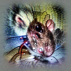
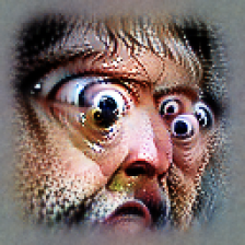
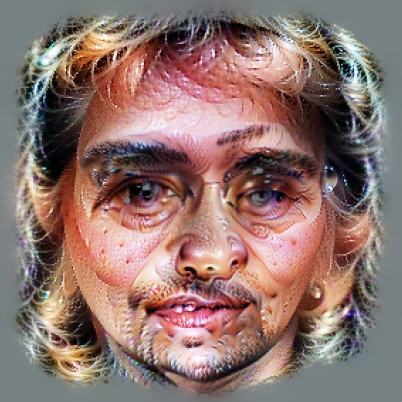
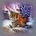
Selected neurons from the final layer of four CLIP models. Each neuron is represented by a feature visualization with a human-chosen concept labels to help quickly provide a sense of each neuron. Labels were picked after looking at hundreds of stimuli that activate the neuron, in addition to feature visualizations. We chose to include some of the examples here to demonstrate the model’s proclivity towards stereotypical depictions of regions, emotions, and other concepts. We also see discrepancies in the level of neuronal resolution: while certain countries like the US and India were associated with well-defined neurons, the same was not true of countries in Africa, where neurons tended to fire for entire regions. We discuss some of these biases and their implications in later sections.

Indeed, we were surprised to find many of these categories appear to mirror neurons in the medial temporal lobe documented in epilepsy patients with intracranial depth electrodes. These include neurons that respond to emotions, animals, and famous people.

But our investigation into CLIP reveals many more such strange and wonderful abstractions, including neurons that appear to count [17, 202, 310], neurons responding to art styles [75, 587, 122], even images with evidence of digital alteration [1640].

Absent concepts

While this analysis shows a great breadth of concepts, we note that a simple analysis on a neuron level cannot represent a complete documentation of the model’s behavior. The authors of CLIP have demonstrated, for example, that the model is capable of very precise geolocation, (Appendix E.4, Figure 20) with a granularity that extends down to the level of a city and even a neighborhood. In fact, we offer an anecdote: we have noticed, by running our own personal photos through CLIP, that CLIP can often recognize if a photo was taken in San Francisco, and sometimes even the neighbourhood (e.g., “Twin Peaks”).

Despite our best efforts, however, we have not found a “San Francisco” neuron, nor did it seem from attribution that San Francisco decomposes nicely into meaningful unit concepts like “California” and “city.” We believe this information to be encoded within the activations of the model somewhere, but in a more exotic way, either as a direction or as some other more complex manifold. We believe this to be a fruitful direction for further research.

How multimodal neurons compose

These multimodal neurons can give us insight into understanding how CLIP performs classification. With a sparse linear probe, we can easily inspect CLIP’s weights to see which concepts combine to achieve a final classification for ImageNet classification:

Multimodal Neurons in Artificial Neural Networks
piggy bank

=
2.5
Multimodal Neurons in Artificial Neural Networks
finance

+
1.1
Multimodal Neurons in Artificial Neural Networks
dolls, toys

+
···

Multimodal Neurons in Artificial Neural Networks
barn spider

=
2.9
Multimodal Neurons in Artificial Neural Networks
Spider-Man

+
1.5
Multimodal Neurons in Artificial Neural Networks
animal

+
···

The piggy bank class appears to be a composition of a “finance” neuron along with a porcelain neuron. The Spider-Man neuron referenced in the first section of the paper is also a spider detector, and plays an important role in the classification of the class “barn spider.”

For text classification, a key observation is that these concepts are contained within neurons in a way that, similar to the word2vec objective, is almost linear. The concepts, therefore, form a simple algebra that behaves similarly to a linear probe. By linearizing the attention, we too can inspect any sentence, much like a linear probe, as shown below:


Multimodal Neurons in Artificial Neural Networks
surprised

=
1.0
Multimodal Neurons in Artificial Neural Networks
celebration, hug

+
1.0
Multimodal Neurons in Artificial Neural Networks
shock

+
0.17
Multimodal Neurons in Artificial Neural Networks
smile, grin

Multimodal Neurons in Artificial Neural Networks
intimate

=
1.0
Multimodal Neurons in Artificial Neural Networks
soft smile

+
0.92
Multimodal Neurons in Artificial Neural Networks
heart

0.8
Multimodal Neurons in Artificial Neural Networks
illness

Probing how CLIP understands words, it appears to the model that the word “surprised” implies some not just some measure of shock, but a shock of a very specific kind, one combined perhaps with delight or wonder. “Intimate” consists of a soft smile and hearts, but not sickness. We note that this reveals a reductive understanding of the the full human experience of intimacy-the subtraction of illness precludes, for example, intimate moments with loved ones who are sick. We find many such omissions when probing CLIP’s understanding of language.

Fallacies of abstraction

The degree of abstraction in CLIP surfaces a new vector of attack that we believe has not manifested in previous systems. Like many deep networks, the representations at the highest layers of the model are completely dominated by such high-level abstractions. What distinguishes CLIP, however, is a matter of degree—CLIP’s multimodal neurons generalize across the literal and the iconic, which may be a double-edged sword.

Through a series of carefully-constructed experiments, we demonstrate that we can exploit this reductive behavior to fool the model into making absurd classifications. We have observed that the excitations of the neurons in CLIP are often controllable by its response to images of text, providing a simple vector of attacking the model.

The finance neuron [1330], for example, responds to images of piggy banks, but also responds to the string “$$$”. By forcing the finance neuron to fire, we can fool our model into classifying a dog as a piggy bank.

Attacks in the wild

We refer to these attacks as typographic attacks. We believe attacks such as those described above are far from simply an academic concern. By exploiting the model’s ability to read text robustly, we find that even photographs of hand-written text can often fool the model. Like the Adversarial Patch, this attack works in the wild; but unlike such attacks, it requires no more technology than pen and paper.

We also believe that these attacks may also take a more subtle, less conspicuous form. An image, given to CLIP, is abstracted in many subtle and sophisticated ways, and these abstractions may over-abstract common patterns—oversimplifying and, by virtue of that, overgeneralizing.

Bias and overgeneralization

Our model, despite being trained on a curated subset of the internet, still inherits its many unchecked biases and associations. Many associations we have discovered appear to be benign, but yet we have discovered several cases where CLIP holds associations that could result in representational harm, such as denigration of certain individuals or groups.

We have observed, for example, a “Middle East” neuron [1895] with an association with terrorism; and an “immigration” neuron [395] that responds to Latin America. We have even found a neuron that fires for both dark-skinned people and gorillas [1257], mirroring earlier photo tagging incidents in other models we consider unacceptable.

These associations present obvious challenges to applications of such powerful visual systems.[1] Whether fine-tuned or used zero-shot, it is likely that these biases and associations will remain in the system, with their effects manifesting in both visible and nearly invisible ways during deployment. Many biased behaviors may be difficult anticipate a priori, making their measurement and correction difficult. We believe that these tools of interpretability may aid practitioners the ability to preempt potential problems, by discovering some of these associations and ambigiuities ahead of time.

Our own understanding of CLIP is still evolving, and we are still determining if and how we would release large versions of CLIP. We hope that further community exploration of the released versions as well as the tools we are announcing today will help advance general understanding of multimodal systems, as well as inform our own decision-making.

Conclusion

Alongside the publication of “Multimodal Neurons in Artificial Neural Networks,” we are also releasing some of the tools we have ourselves used to understand CLIP—the OpenAI Microscope catalog has been updated with feature visualizations, dataset examples, and text feature visualizations for every neuron in CLIP RN50x4. We are also releasing the weights of CLIP RN50x4 and RN101 to further accommodate such research. We believe these investigations of CLIP only scratch the surface in understanding CLIP’s behavior, and we invite the research community to in improving our understanding of CLIP and models like it.

OpenAI

GFN Thursday — 21 Games Coming to GeForce NOW in March

Guess what’s back? Back again? GFN Thursday. Tell a friend.

Check out this month’s list of all the exciting new titles and classic games coming to GeForce NOW in March.

First, let’s get into what’s coming today.

Don’t Hesitate

It wouldn’t be GFN Thursday if members didn’t have new games to play. Here’s what’s new to GFN starting today:

Loop Hero on GeForce NOW

Loop Hero (day-and-date release on Steam)

Equal parts roguelike, deck-builder and auto battler, Loop Hero challenges you to think strategically as you explore each randomly generated loop path and fight to defeat The Lich. PC Gamer gave this indie high praise, saying, “don’t sleep on this brilliant roguelike.”

Disgaea PC on GeForce NOW

Disgaea PC (Steam)

The turn-based strategy RPG classic lets you amass your evil hordes and become the new Overlord. With more than 40 character types and PC-specific features, there’s never been a better time to visit the Netherworld.

Members can also look for the following games joining GeForce NOW later today:

  • Legends of Aria (Steam)
  • The Dungeon Of Naheulbeuk: The Amulet Of Chaos (Steam)
  • Wargame: Red Dragon (Free on Epic Games Store, March 4-11)
  • WRC 8 FIA World Rally Championship (Steam)

What’s Coming in March

We’ve got a great list of exciting tiles coming soon to GeForce NOW. You won’t want to miss:

Spacebase Startopia (Steam and Epic Games Store)

An original mixture of economic simulation and empire building strategy paired with classic RTS skirmishes and a good dose of humor to take the edge off.

Wrench (Steam)

Prepare and maintain race cars in an extraordinarily detailed mechanic simulator. Extreme attention has been paid to even the smallest components, including fasteners that are accurate to the thread pitch and install torque.

And that’s not all — check out even more games coming to GFN in March:

  • Door Kickers (Steam)
  • Endzone – A World Apart (Steam)
  • Monopoly Plus (Steam)
  • Monster Energy Supercross – The Official Videogame 4 (Steam)
  • Narita Boy (Steam)
  • Overcooked!: All You Can Eat (Steam)
  • Pascal’s Wager – Definitive Edition (Steam)
  • System Shock: Enhanced Edition (Steam)
  • Thief Gold (Steam)
  • Trackmania United Forever (Steam)
  • Uno (Steam)
  • Workers & Resources: Soviet Republic (Steam)
  • Worms Reloaded (Steam)

In Case You Missed It

Remember that one time in February when we told you that 30 titles were coming to GeForce NOW? Actually, it was even more than that — 18 additional games joined the service, bringing the total in February to nearly 50.

If you’re not following along every week, the additional 18 games that joined GFN are:

Add it all up, and you’ve got a lot of gaming ahead of you.

The Backbone of Your GFN iOS Experience

Backbone One, a GeForce NOW Recommended Controller

For those planning to give our new Safari iOS experience a try, our newest GeForce NOW Recommended Controller is for you.

Backbone One is an iPhone game controller recommended for GeForce NOW, with fantastic buttons and build quality, technology that preserves battery life and reduces latency, passthrough charging and more. It even has a built-in capture button to let you record and share your gameplay, right from your phone. Learn more about Backbone One on the GeForce NOW Recommended Product hub.

This should be an exciting month, GFN members. What are you going to play? Tell us on Twitter or in the comments below.

The post GFN Thursday — 21 Games Coming to GeForce NOW in March appeared first on The Official NVIDIA Blog.

Read More

The torch.fft module: Accelerated Fast Fourier Transforms with Autograd in PyTorch

The Fast Fourier Transform (FFT) calculates the Discrete Fourier Transform in O(n log n) time. It is foundational to a wide variety of numerical algorithms and signal processing techniques since it makes working in signals’ “frequency domains” as tractable as working in their spatial or temporal domains.

As part of PyTorch’s goal to support hardware-accelerated deep learning and scientific computing, we have invested in improving our FFT support, and with PyTorch 1.8, we are releasing the torch.fft module. This module implements the same functions as NumPy’s np.fft module, but with support for accelerators, like GPUs, and autograd.

Getting started

Getting started with the new torch.fft module is easy whether you are familiar with NumPy’s np.fft module or not. While complete documentation for each function in the module can be found here, a breakdown of what it offers is:

  • fft, which computes a complex FFT over a single dimension, and ifft, its inverse
  • the more general fftn and ifftn, which support multiple dimensions
  • The “real” FFT functions, rfft, irfft, rfftn, irfftn, designed to work with signals that are real-valued in their time domains
  • The “Hermitian” FFT functions, hfft and ihfft, designed to work with signals that are real-valued in their frequency domains
  • Helper functions, like fftfreq, rfftfreq, fftshift, ifftshift, that make it easier to manipulate signals

We think these functions provide a straightforward interface for FFT functionality, as vetted by the NumPy community, although we are always interested in feedback and suggestions!

To better illustrate how easy it is to move from NumPy’s np.fft module to PyTorch’s torch.fft module, let’s look at a NumPy implementation of a simple low-pass filter that removes high-frequency variance from a 2-dimensional image, a form of noise reduction or blurring:

import numpy as np
import numpy.fft as fft

def lowpass_np(input, limit):
    pass1 = np.abs(fft.rfftfreq(input.shape[-1])) < limit
    pass2 = np.abs(fft.fftfreq(input.shape[-2])) < limit
    kernel = np.outer(pass2, pass1)
    
    fft_input = fft.rfft2(input)
    return fft.irfft2(fft_input * kernel, s=input.shape[-2:])

Now let’s see the same filter implemented in PyTorch:

import torch
import torch.fft as fft

def lowpass_torch(input, limit):
    pass1 = torch.abs(fft.rfftfreq(input.shape[-1])) < limit
    pass2 = torch.abs(fft.fftfreq(input.shape[-2])) < limit
    kernel = torch.outer(pass2, pass1)
    
    fft_input = fft.rfft2(input)
    return fft.irfft2(fft_input * kernel, s=input.shape[-2:])

Not only do current uses of NumPy’s np.fft module translate directly to torch.fft, the torch.fft operations also support tensors on accelerators, like GPUs and autograd. This makes it possible to (among other things) develop new neural network modules using the FFT.

Performance

The torch.fft module is not only easy to use — it is also fast! PyTorch natively supports Intel’s MKL-FFT library on Intel CPUs, and NVIDIA’s cuFFT library on CUDA devices, and we have carefully optimized how we use those libraries to maximize performance. While your own results will depend on your CPU and CUDA hardware, computing Fast Fourier Transforms on CUDA devices can be many times faster than computing it on the CPU, especially for larger signals.

In the future, we may add support for additional math libraries to support more hardware. See below for where you can request additional hardware support.

Updating from older PyTorch versions

Some PyTorch users might know that older versions of PyTorch also offered FFT functionality with the torch.fft() function. Unfortunately, this function had to be removed because its name conflicted with the new module’s name, and we think the new functionality is the best way to use the Fast Fourier Transform in PyTorch. In particular, torch.fft() was developed before PyTorch supported complex tensors, while the torch.fft module was designed to work with them.

PyTorch also has a “Short Time Fourier Transform”, torch.stft, and its inverse torch.istft. These functions are being kept but updated to support complex tensors.

Future

As mentioned, PyTorch 1.8 offers the torch.fft module, which makes it easy to use the Fast Fourier Transform (FFT) on accelerators and with support for autograd. We encourage you to try it out!

While this module has been modeled after NumPy’s np.fft module so far, we are not stopping there. We are eager to hear from you, our community, on what FFT-related functionality you need, and we encourage you to create posts on our forums at https://discuss.pytorch.org/, or file issues on our Github with your feedback and requests. Early adopters have already started asking about Discrete Cosine Transforms and support for more hardware platforms, for example, and we are investigating those features now.

We look forward to hearing from you and seeing what the community does with PyTorch’s new FFT functionality!

Read More

PyTorch 1.8 Release, including Compiler and Distributed Training updates, and New Mobile Tutorials

We are excited to announce the availability of PyTorch 1.8. This release is composed of more than 3,000 commits since 1.7. It includes major updates and new features for compilation, code optimization, frontend APIs for scientific computing, and AMD ROCm support through binaries that are available via pytorch.org. It also provides improved features for large-scale training for pipeline and model parallelism, and gradient compression. A few of the highlights include:

  1. Support for doing python to python functional transformations via torch.fx;
  2. Added or stabilized APIs to support FFTs (torch.fft), Linear Algebra functions (torch.linalg), added support for autograd for complex tensors and updates to improve performance for calculating hessians and jacobians; and
  3. Significant updates and improvements to distributed training including: Improved NCCL reliability; Pipeline parallelism support; RPC profiling; and support for communication hooks adding gradient compression.
    See the full release notes here.

Along with 1.8, we are also releasing major updates to PyTorch libraries including TorchCSPRNG, TorchVision, TorchText and TorchAudio. For more on the library releases, see the post here. As previously noted, features in PyTorch releases are classified as Stable, Beta and Prototype. You can learn more about the definitions in the post here.

New and Updated APIs

The PyTorch 1.8 release brings a host of new and updated API surfaces ranging from additional APIs for NumPy compatibility, also support for ways to improve and scale your code for performance at both inference and training time. Here is a brief summary of the major features coming in this release:

[Stable] Torch.fft support for high performance NumPy style FFTs

As part of PyTorch’s goal to support scientific computing, we have invested in improving our FFT support and with PyTorch 1.8, we are releasing the torch.fft module. This module implements the same functions as NumPy’s np.fft module, but with support for hardware acceleration and autograd.

[Beta] Support for NumPy style linear algebra functions via torch.linalg

The torch.linalg module, modeled after NumPy’s np.linalg module, brings NumPy-style support for common linear algebra operations including Cholesky decompositions, determinants, eigenvalues and many others.

[Beta] Python code Transformations with FX

FX allows you to write transformations of the form transform(input_module : nn.Module) -> nn.Module, where you can feed in a Module instance and get a transformed Module instance out of it.

This kind of functionality is applicable in many scenarios. For example, the FX-based Graph Mode Quantization product is releasing as a prototype contemporaneously with FX. Graph Mode Quantization automates the process of quantizing a neural net and does so by leveraging FX’s program capture, analysis and transformation facilities. We are also developing many other transformation products with FX and we are excited to share this powerful toolkit with the community.

Because FX transforms consume and produce nn.Module instances, they can be used within many existing PyTorch workflows. This includes workflows that, for example, train in Python then deploy via TorchScript.

Below is an FX transform example:

import torch
import torch.fx

def transform(m: nn.Module,
             tracer_class : type = torch.fx.Tracer) -> torch.nn.Module:
   # Step 1: Acquire a Graph representing the code in `m`
  
   # NOTE: torch.fx.symbolic_trace is a wrapper around a call to
   # fx.Tracer.trace and constructing a GraphModule. We'll
   # split that out in our transform to allow the caller to
   # customize tracing behavior.
   graph : torch.fx.Graph = tracer_class().trace(m)
  
   # Step 2: Modify this Graph or create a new one
   graph = ...
  
   # Step 3: Construct a Module to return
   return torch.fx.GraphModule(m, graph)

You can read more about FX in the official documentation. You can also find several examples of program transformations implemented using torch.fx here. We are constantly improving FX and invite you to share any feedback you have about the toolkit on the forums or issue tracker.

Distributed Training

The PyTorch 1.8 release added a number of new features as well as improvements to reliability and usability. Concretely, support for: Stable level async error/timeout handling was added to improve NCCL reliability; and stable support for RPC based profiling. Additionally, we have added support for pipeline parallelism as well as gradient compression through the use of communication hooks in DDP. Details are below:

[Beta] Pipeline Parallelism

As machine learning models continue to grow in size, traditional Distributed DataParallel (DDP) training no longer scales as these models don’t fit on a single GPU device. The new pipeline parallelism feature provides an easy to use PyTorch API to leverage pipeline parallelism as part of your training loop.

[Beta] DDP Communication Hook

The DDP communication hook is a generic interface to control how to communicate gradients across workers by overriding the vanilla allreduce in DistributedDataParallel. A few built-in communication hooks are provided including PowerSGD, and users can easily apply any of these hooks to optimize communication. Additionally, the communication hook interface can also support user-defined communication strategies for more advanced use cases.

Additional Prototype Features for Distributed Training

In addition to the major stable and beta distributed training features in this release, we also have a number of prototype features available in our nightlies to try out and provide feedback. We have linked in the draft docs below for reference:

  • (Prototype) ZeroRedundancyOptimizer – Based on and in partnership with the Microsoft DeepSpeed team, this feature helps reduce per-process memory footprint by sharding optimizer states across all participating processes in the ProcessGroup gang. Refer to this documentation for more details.
  • (Prototype) Process Group NCCL Send/Recv – The NCCL send/recv API was introduced in v2.7 and this feature adds support for it in NCCL process groups. This feature will provide an option for users to implement collective operations at Python layer instead of C++ layer. Refer to this documentation and code examples to learn more.
  • (Prototype) CUDA-support in RPC using TensorPipe – This feature should bring consequent speed improvements for users of PyTorch RPC with multiple-GPU machines, as TensorPipe will automatically leverage NVLink when available, and avoid costly copies to and from host memory when exchanging GPU tensors between processes. When not on the same machine, TensorPipe will fall back to copying the tensor to host memory and sending it as a regular CPU tensor. This will also improve the user experience as users will be able to treat GPU tensors like regular CPU tensors in their code. Refer to this documentation for more details.
  • (Prototype) Remote Module – This feature allows users to operate a module on a remote worker like using a local module, where the RPCs are transparent to the user. In the past, this functionality was implemented in an ad-hoc way and overall this feature will improve the usability of model parallelism on PyTorch. Refer to this documentation for more details.

PyTorch Mobile

Support for PyTorch Mobile is expanding with a new set of tutorials to help new users launch models on-device quicker and give existing users a tool to get more out of our framework. These include:

Our new demo apps also include examples of image segmentation, object detection, neural machine translation, question answering, and vision transformers. They are available on both iOS and Android:

In addition to performance improvements on CPU for MobileNetV3 and other models, we also revamped our Android GPU backend prototype for broader models coverage and faster inferencing:

Lastly, we are launching the PyTorch Mobile Lite Interpreter as a prototype feature in this release. The Lite Interpreter allows users to reduce the runtime binary size. Please try these out and send us your feedback on the PyTorch Forums. All our latest updates can be found on the PyTorch Mobile page

[Prototype] PyTorch Mobile Lite Interpreter

PyTorch Lite Interpreter is a streamlined version of the PyTorch runtime that can execute PyTorch programs in resource constrained devices, with reduced binary size footprint. This prototype feature reduces binary sizes by up to 70% compared to the current on-device runtime in the current release.

Performance Optimization

In 1.8, we are releasing the support for benchmark utils to enable users to better monitor performance. We are also opening up a new automated quantization API. See the details below:

(Beta) Benchmark utils

Benchmark utils allows users to take accurate performance measurements, and provides composable tools to help with both benchmark formulation and post processing. This expected to be helpful for contributors to PyTorch to quickly understand how their contributions are impacting PyTorch performance.

Example:

from torch.utils.benchmark import Timer

results = []
for num_threads in [1, 2, 4]:
    timer = Timer(
        stmt="torch.add(x, y, out=out)",
        setup="""
            n = 1024
            x = torch.ones((n, n))
            y = torch.ones((n, 1))
            out = torch.empty((n, n))
        """,
        num_threads=num_threads,
    )
    results.append(timer.blocked_autorange(min_run_time=5))
    print(
        f"{num_threads} thread{'s' if num_threads > 1 else ' ':<4}"
        f"{results[-1].median * 1e6:>4.0f} us   " +
        (f"({results[0].median / results[-1].median:.1f}x)" if num_threads > 1 else '')
    )

1 thread     376 us   
2 threads    189 us   (2.0x)
4 threads     99 us   (3.8x)

(Prototype) FX Graph Mode Quantization

FX Graph Mode Quantization is the new automated quantization API in PyTorch. It improves upon Eager Mode Quantization by adding support for functionals and automating the quantization process, although people might need to refactor the model to make the model compatible with FX Graph Mode Quantization (symbolically traceable with torch.fx).

Hardware Support

[Beta] Ability to Extend the PyTorch Dispatcher for a new backend in C++

In PyTorch 1.8, you can now create new out-of-tree devices that live outside the pytorch/pytorch repo. The tutorial linked below shows how to register your device and keep it in sync with native PyTorch devices.

[Beta] AMD GPU Binaries Now Available

Starting in PyTorch 1.8, we have added support for ROCm wheels providing an easy onboarding to using AMD GPUs. You can simply go to the standard PyTorch installation selector and choose ROCm as an installation option and execute the provided command.

Thanks for reading, and if you are excited about these updates and want to participate in the future of PyTorch, we encourage you to join the discussion forums and open GitHub issues.

Cheers!

Team PyTorch

Read More

New PyTorch library releases including TorchVision Mobile, TorchAudio I/O, and more

Today, we are announcing updates to a number of PyTorch libraries, alongside the PyTorch 1.8 release. The updates include new releases for the domain libraries including TorchVision, TorchText and TorchAudio as well as new version of TorchCSPRNG. These releases include a number of new features and improvements and, along with the PyTorch 1.8 release, provide a broad set of updates for the PyTorch community to build on and leverage.

Some highlights include:

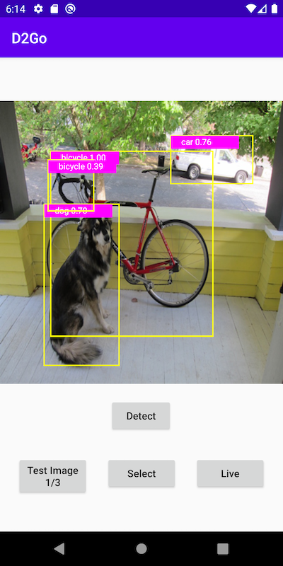
  • TorchVision – Added support for PyTorch Mobile including Detectron2Go (D2Go), auto-augmentation of data during training, on the fly type conversion, and AMP autocasting.
  • TorchAudio – Major improvements to I/O, including defaulting to sox_io backend and file-like object support. Added Kaldi Pitch feature and support for CMake based build allowing TorchAudio to better support no-Python environments.
  • TorchText – Updated the dataset loading API to be compatible with standard PyTorch data loading utilities.
  • TorchCSPRNG – Support for cryptographically secure pseudorandom number generators for PyTorch is now stable with new APIs for AES128 ECB/CTR and CUDA support on Windows.

Please note that, starting in PyTorch 1.6, features are classified as Stable, Beta, and Prototype. Prototype features are not included as part of the binary distribution and are instead available through either building from source, using nightlies or via compiler flag. You can see the detailed announcement here.

TorchVision 0.9.0

[Stable] TorchVision Mobile: Operators, Android Binaries, and Tutorial

We are excited to announce the first on-device support and binaries for a PyTorch domain library. We have seen significant appetite in both research and industry for on-device vision support to allow low latency, privacy friendly, and resource efficient mobile vision experiences. You can follow this new tutorial to build your own Android object detection app using TorchVision operators, D2Go, or your own customer operators and model.

[Stable] New Mobile models for Classification, Object Detection and Semantic Segmentation

We have added support for the MobileNetV3 architecture and provided pre-trained weights for Classification, Object Detection and Segmentation. It is easy to get up and running with these models, just import and load them as you would any torchvision model:

import torch
import torchvision

# Classification
x = torch.rand(1, 3, 224, 224)
m_classifier = torchvision.models.mobilenet_v3_large(pretrained=True)
m_classifier.eval()
predictions = m_classifier(x)

# Quantized Classification
x = torch.rand(1, 3, 224, 224)
m_classifier = torchvision.models.quantization.mobilenet_v3_large(pretrained=True)
m_classifier.eval()
predictions = m_classifier(x)

# Object Detection: Highly Accurate High Resolution Mobile Model
x = [torch.rand(3, 300, 400), torch.rand(3, 500, 400)]
m_detector = torchvision.models.detection.fasterrcnn_mobilenet_v3_large_fpn(pretrained=True)
m_detector.eval()
predictions = m_detector(x)

# Semantic Segmentation: Highly Accurate Mobile Model
x = torch.rand(1, 3, 520, 520)
m_segmenter = torchvision.models.segmentation.deeplabv3_mobilenet_v3_large(pretrained=True)
m_segmenter.eval()
predictions = m_segmenter(x)

These models are highly competitive with TorchVision’s existing models on resource efficiency, speed, and accuracy. See our release notes for detailed performance metrics.

[Stable] AutoAugment

AutoAugment is a common Data Augmentation technique that can increase the accuracy of Scene Classification models. Though the data augmentation policies are directly linked to their trained dataset, empirical studies show that ImageNet policies provide significant improvements when applied to other datasets. We’ve implemented 3 policies learned on the following datasets: ImageNet, CIFA10 and SVHN. These can be used standalone or mixed-and-matched with existing transforms:

from torchvision import transforms

t = transforms.AutoAugment()
transformed = t(image)


transform=transforms.Compose([
   transforms.Resize(256),
   transforms.AutoAugment(),
   transforms.ToTensor()])

Other New Features for TorchVision

  • [Stable] All read and decode methods in the io.image package now support:
    • Palette, Grayscale Alpha and RBG Alpha image types during PNG decoding
    • On-the-fly conversion of image from one type to the other during read
  • [Stable] WiderFace dataset
  • [Stable] Improved FasterRCNN speed and accuracy by introducing a score threshold on RPN
  • [Stable] Modulation input for DeformConv2D
  • [Stable] Option to write audio to a video file
  • [Stable] Utility to draw bounding boxes
  • [Beta] Autocast support in all Operators
    Find the full TorchVision release notes here.

TorchAudio 0.8.0

I/O Improvements

We have continued our work from the previous release to improve TorchAudio’s I/O support, including:

  • [Stable] Changing the default backend to “sox_io” (for Linux/macOS), and updating the “soundfile” backend’s interface to align with that of “sox_io”. The legacy backend and interface are still accessible, though it is strongly discouraged to use them.
  • [Stable] File-like object support in both “sox_io” backend, “soundfile” backend and sox_effects.
  • [Stable] New options to change the format, encoding, and bits_per_sample when saving.
  • [Stable] Added GSM, HTK, AMB, AMR-NB and AMR-WB format support to the “sox_io” backend.
  • [Beta] A new functional.apply_codec function which can degrade audio data by applying audio codecs supported by “sox_io” backend in an in-memory fashion.
    Here are some examples of features landed in this release:
# Load audio over HTTP
with requests.get(URL, stream=True) as response:
    waveform, sample_rate = torchaudio.load(response.raw)
 
# Saving to Bytes buffer as 32-bit floating-point PCM
buffer_ = io.BytesIO()
torchaudio.save(
    buffer_, waveform, sample_rate,
    format="wav", encoding="PCM_S", bits_per_sample=16)
 
# Apply effects while loading audio from S3
client = boto3.client('s3')
response = client.get_object(Bucket=S3_BUCKET, Key=S3_KEY)
waveform, sample_rate = torchaudio.sox_effects.apply_effect_file(
    response['Body'],
    [["lowpass", "-1", "300"], ["rate", "8000"]])
 
# Apply GSM codec to Tensor
encoded = torchaudio.functional.apply_codec(
    waveform, sample_rate, format="gsm")

Check out the revamped audio preprocessing tutorial, Audio Manipulation with TorchAudio.

[Stable] Switch to CMake-based build

In the previous version of TorchAudio, it was utilizing CMake to build third party dependencies. Starting in 0.8.0, TorchaAudio uses CMake to build its C++ extension. This will open the door to integrate TorchAudio in non-Python environments (such as C++ applications and mobile). We will continue working on adding example applications and mobile integrations.

[Beta] Improved and New Audio Transforms

We have added two widely requested operators in this release: the SpectralCentroid transform and the Kaldi Pitch feature extraction (detailed in “A pitch extraction algorithm tuned for automatic speech recognition”). We’ve also exposed a normalization method to Mel transforms, and additional STFT arguments to Spectrogram. We would like to ask our community to continue to raise feature requests for core audio processing features like these!

Community Contributions

We had more contributions from the open source community in this release than ever before, including several completely new features. We would like to extend our sincere thanks to the community. Please check out the newly added CONTRIBUTING.md for ways to contribute code, and remember that reporting bugs and requesting features are just as valuable. We will continue posting well-scoped work items as issues labeled “help-wanted” and “contributions-welcome” for anyone who would like to contribute code, and are happy to coach new contributors through the contribution process.

Find the full TorchAudio release notes here.

TorchText 0.9.0

[Beta] Dataset API Updates

In this release, we are updating TorchText’s dataset API to be compatible with PyTorch data utilities, such as DataLoader, and are deprecating TorchText’s custom data abstractions such as Field. The updated datasets are simple string-by-string iterators over the data. For guidance about migrating from the legacy abstractions to use modern PyTorch data utilities, please refer to our migration guide.

The text datasets listed below have been updated as part of this work. For examples of how to use these datasets, please refer to our end-to-end text classification tutorial.

  • Language modeling: WikiText2, WikiText103, PennTreebank, EnWik9
  • Text classification: AG_NEWS, SogouNews, DBpedia, YelpReviewPolarity, YelpReviewFull, YahooAnswers, AmazonReviewPolarity, AmazonReviewFull, IMDB
  • Sequence tagging: UDPOS, CoNLL2000Chunking
  • Translation: IWSLT2016, IWSLT2017
  • Question answer: SQuAD1, SQuAD2

Find the full TorchText release notes here.

[Stable] TorchCSPRNG 0.2.0

We released TorchCSPRNG in August 2020, a PyTorch C++/CUDA extension that provides cryptographically secure pseudorandom number generators for PyTorch. Today, we are releasing the 0.2.0 version and designating the library as stable. This release includes a new API for encrypt/decrypt with AES128 ECB/CTR as well as CUDA 11 and Windows CUDA support.

Find the full TorchCSPRNG release notes here.

Thanks for reading, and if you are excited about these updates and want to participate in the future of PyTorch, we encourage you to join the discussion forums and open GitHub issues.

Cheers!

Team PyTorch

Read More

Utilizing XGBoost training reports to improve your models

In 2019, AWS unveiled Amazon SageMaker Debugger, a SageMaker capability that enables you to automatically detect a variety of issues that may arise while a model is being trained. SageMaker Debugger captures model state data at specified intervals during a training job. With this data, SageMaker Debugger can detect training issues or anomalies by leveraging built-in or user-defined rules. In addition to detecting issues during the training job, you can analyze the captured state data afterwards to evaluate model performance and identify areas for improvement. This task is made easier with the newly launched XGBoost training report feature. With a minimal amount of code changes, SageMaker Debugger generates a comprehensive report outlining key information that you can use to evaluate and improve the model.

This post shows you an end-to-end example of training an XGBoost model on Sagemaker and how to enable the automatic XGBoost report functionality in Sagemaker Debugger to quickly and easily evaluate model performance and identify areas of improvement for your model. Even if you don’t have a lot of data science experience, you can still gauge how well the model performs and identify areas of improvement based on information provided by the report. The code from this post is available in the GitHub repo.

Dataset

For this example, we use the dataset from the Kaggle ATLAS Higgs Boson Machine Learning Challenge 2014. With this dataset, we train a machine learning (ML) model to automatically classify Higgs Boson events from others (such as background noise) generated from simulated proton-proton collisions in CERN’s Large Hadron Collider. The data can be obtained directly from CERN. Let’s go through the steps of obtaining the data and configuring the training job. You can follow along with a Jupyter notebook.

  1. We start with the relevant imports:
    import requests
    from io import BytesIO
    import pandas as pd
    import boto3
    import s3fs
    from datetime import datetime
    import time
    import sagemaker
    from sagemaker.estimator import Estimator
    from sagemaker import image_uris
    from sagemaker.inputs import TrainingInput
    from sagemaker.debugger import Rule, rule_configs
    
    from IPython.display import FileLink, FileLinks
    

  1. Then we set up variables that we later need to configure the SageMaker training job:
    # setup sagemaker variables
    role = sagemaker.get_execution_role()
    sess = sagemaker.session.Session()
    bucket = sess.default_bucket()
    key_prefix = "higgs-boson"
    region = sess._region_name
    s3 = s3fs.S3FileSystem(anon=False)
    xgboost_container = image_uris.retrieve("xgboost", region, "1.2-1")
    

  1. We obtain data and prepare it for training:
    # obtain data from CERN and load it into a DataFrame
    data_url = "http://opendata.cern.ch/record/328/files/atlas-higgs-challenge-2014-v2.csv.gz"
    gz_file = BytesIO(requests.get(data_url).content)
    gz_file.flush()
    df = pd.read_csv(gz_file, compression="gzip")
    
    # identify feature, label, and unused columns
    non_feature_cols = ["EventId", "Weight", "KaggleSet", "KaggleWeight", "Label"]
    feature_cols = [col for col in df.columns if col not in non_feature_cols]
    label_col = "Label"
    df["Label"] = df["Label"].apply(lambda x: 1 if x=="s" else 0)
    
    # take subsets of data per the original Kaggle competition
    train_data = df.loc[df["KaggleSet"] == "t", [label_col, *feature_cols]]
    test_data = df.loc[df["KaggleSet"] == "b", [label_col, *feature_cols]]
    
    # upload data to S3
    for name, dataset in zip(["train", "test"], [train_data, test_data]):
        sess.upload_string_as_file_body(body=dataset.to_csv(index=False, header=False),
                                       bucket=bucket,
                                       key=f"{key_prefix}/input/{name}.csv"
                                       )
                                       
    # configure data inputs for SageMaker training
    train_input = TrainingInput(f"s3://{bucket}/{key_prefix}/input/train.csv", content_type="text/csv")
    validation_input = TrainingInput(f"s3://{bucket}/{key_prefix}/input/test.csv", content_type="text/csv")
    

Setting up a training job with XGBoost training report

We only need to make one code change to the typical process for launching a training job: adding the create_xgboost_report rule to the Estimator. SageMaker takes care of the rest. A companion SageMaker processing job spins up to analyze the XGBoost model and produce the report. This analysis is done at no additional cost. See the following additional code:

# add a rule to generate the XGBoost Report
rules=[
    Rule.sagemaker(rule_configs.create_xgboost_report())
]

hyperparameters={
    "max_depth": "6",
    "eta": "0.1",
    "objective": "binary:logistic",
    "num_round": "100",
    
}

estimator=Estimator(
    role=role,
    image_uri=xgboost_container,
    base_job_name="higgs-boson-model",
    instance_count=1,
    instance_type="ml.m5.2xlarge",
    hyperparameters=hyperparameters,
    rules=rules, 
)

training_job_time = datetime.now()
estimator.fit({'train': train_input, 'validation': validation_input}, 
              wait=True)

Analyzing models with the XGBoost training report

When the training job is complete, SageMaker automatically starts the processing job to generate the XGBoost report. We write a few lines of code to check the status of the processing job. When it’s complete, we download it to our local drive for further review. The following code downloads the report upon its completion, and provides a hyperlink directly within the notebook for easy viewing:

import os
#get name of profiler report
profiler_report_name = [rule["RuleConfigurationName"] 
                        for rule in estimator.latest_training_job.rule_job_summary() 
                        if "Profiler" in rule["RuleConfigurationName"]][0]

xgb_profile_job_name = [rule["RuleEvaluationJobArn"].split("/")[-1] 
                        for rule in estimator.latest_training_job.rule_job_summary() 
                        if "CreateXgboostReport" in rule["RuleConfigurationName"]][0]

base_output_path = os.path.dirname(estimator.latest_job_debugger_artifacts_path())
rule_output_path = os.path.join(base_output_path, "rule-output/")
xgb_report_path = os.path.join(rule_output_path, "CreateXgboostReport")
profile_report_path = os.path.join(rule_output_path, profiler_report_name)

while True:
    
    xgb_job_info = sess.sagemaker_client.describe_processing_job(ProcessingJobName=xgb_profile_job_name)

    if xgb_job_info["ProcessingJobStatus"] == "Completed":
        break
    else:
        print(f"Job Status: {xgb_job_info['ProcessingJobStatus']}")
        time.sleep(30)

s3.download(xgb_report_path, "reports/xgb/", recursive=True)
s3.download(profile_report_path, "reports/profiler/", recursive=True)
display("Click link below to view the profiler report", FileLink("reports/profiler/profiler-output/profiler-report.html"))
display("Click link below to view the XGBoost Training report", FileLink("reports/xgb/xgboost_report.html"))

Before we dive into the training report, let’s take a quick look at the SageMaker Debugger report, which by default is generated after every training job. This report provides key metrics around resource utilization such as network, I/O, and CPU. In the following example, we can see the median CPU utilization was at around 55% while memory utilization was consistently under 5%. This tells us that we can reduce costs by utilizing a smaller training instance.

This report provides key metrics around resource utilization such as network, I/O, and CPU.

Now let’s dive into the training report. SageMaker Debugger automatically generates the following key insights on our model:

  • Distribution of labels – Detects imbalanced datasets
  • Loss graph – Detects over-fitting or over training
  • Feature importance metrics – Identifies redundant or uninformative features
  • Confusion matrix and evaluation metrics – Evaluates performance at the individual class level and identifies concentrations of errors
  • Accuracy rate per iteration – Shows how accuracy improved for each class over each round of boosting
  • Receiver operating characteristic curve – Shows how the model performs under different probability thresholds
  • Distribution of residuals – Helps determine if residuals are a result of random error or missing information

We pick a few items from the report for demonstration purposes.

Distribution of true labels of the dataset

This visualization shows the distribution of labeled classes (for classification) or values (for regression) in your original dataset. An imbalanced dataset could result in poor predictive performance unless properly handled. In this particular example, there’s a slight imbalance between the negative and positive label.

This visualization shows the distribution of labeled classes (for classification) or values (for regression) in your original dataset.Loss vs. step graph

This visualization compares the loss from the training dataset against the validation dataset. For this particular model, it looks like this model is over-fitting on the training set because the validation error remains relatively flat after about 30 boosting rounds, even though the error on the training loss continues to improve.

This visualization compares the loss from the training dataset against the validation dataset

Feature importance

This visualization shows you feature importance by weight, gain, and coverage. Gain, which measures the relative contribution of each feature, is typically the most relevant one for most use cases. For this particular model, we see that a handful of features provide the bulk of the contribution, while a large number contribute little to no gain to the model’s predictive performance. It’s usually a good practice to drop uninformative features from the model because they add noise and may result in over-fitting.

This visualization shows you feature importance by weight, gain, and coverage.

Confusion matrix and ROC curve

There are a number of additional visualizations that show you the common things data scientists often look at, such as the confusion matrix, ROC curve, and F1 score. For more information, see Debugger XGBoost Training Report Walkthrough.

From the following confusion matrix, we can see that the model does a better job at predicting for class 0 than class 1. And this can be explained by the imbalanced label distribution we showed at the beginning (there are more instances for class 0 than class 1). One ramification is making the label distribution more balanced via data resampling techniques.

From the following confusion matrix, we can see that the model does a better job at predicting for class 0 than class 1.

SageMaker Debugger automatically generates and reports the performance metrics such as F1 score and accuracy. You can also see a classification report, such as the following.

You can also see a classification report, such as the following.

Fine-tuning performance

From the training report’s outputs, we can see several areas where the model can be fine-tuned to improve performance, notably the following:

  • The loss vs. step graph indicates that the validation error stopped improving after about 30 rounds, so we can reduce the number of boosting rounds or enable early stopping to mitigate over-training.
  • The feature importance graph shows a large number of uninformative features that could potentially be removed to reduce over-fitting and improve predictive performance on unseen datasets.
  • Based on the confusion matrix and the classification report, the recall score is somewhat low, meaning we’ve misclassified a large number of signal events. Tuning the scale_pos_weight parameter to adjust for the imbalance in the dataset could help improve this.

Conclusion

In this post, we generated an XGBoost training report and profiler report using SageMaker Debugger. With these, we got reports for both the model performance and the resource utilization during training automatically. We then walked through the XGBoost training report and identified a number of issues that we can alleviate with some hyperparameter tuning.

For more about SageMaker Debugger, see SageMaker Debugger XGBoost Training Report and SageMaker Debugger Profiling Report.


About the Authors

Simon ZamarinSimon Zamarin is an AI/ML Solutions Architect whose main focus is helping customers extract value from their data assets. In his spare time, Simon enjoys spending time with family, reading sci-fi, and working on various DIY house projects.


Lu HuangLu Huang is a Senior Product Manager on the AWS Deep Engine team, managing Sagemaker Debugger.


Satadal Bhattacharjee is Principal Product Manager at AWS AI. He leads the machine learning engine PM team on projects such as SageMaker and optimizes machine learning frameworks such as TensorFlow, PyTorch, and MXNet.


Qingwei Li is a Machine Learning Specialist at Amazon Web Services. He received his Ph.D. in Operations Research after he broke his advisor’s research grant account and failed to deliver the Nobel Prize he promised. Currently he helps customers in the financial service and insurance industry build machine learning solutions on AWS. In his spare time, he likes reading and teaching.


Nihal HarishNihal Harish is an engineer at AWS AI. He loves working at the intersection of distributed systems and machine learning. Outside of work, he enjoys long distance running and playing tennis.

Read More

A Tour of SavedModel Signatures

Posted by Daniel Ellis, TensorFlow Engineer

Note: This blog post is aimed at TensorFlow developers who want to learn the details of how graphs and models are stored. If you are new to TensorFlow, you should check out the TensorFlow Basics guides before reading this article.

TensorFlow can run models without the original Python objects, as demonstrated by TensorFlow Serving and TensorFlow Lite, or when you download a trained model from TensorFlow Hub.

Models and layers can be loaded from this representation without actually making an instance of the Python class that created it. This is desired in situations where you do not have (or want) a Python interpreter, such as serving at scale or on an edge device, or in situations where the original Python code is not available.

Saved models are represented by two separate, but equally important, parts: the graph, which describes the fixed computation described in code, and the weights, which are the dynamic parameters you trained during training. If you aren’t already familiar with this and @tf.function, you should check out the Introduction to graphs and functions guide as well as the section on saving in the modules, layers, and models guide.

From a code standpoint, functions decorated with @tf.function create a Python callable; in the documentation we refer to these as polymorphic functions, as they are Python callables that can take a variety argument signatures. Each time you call a @tf.function with a new argument signature, TensorFlow traces out a new graph just for that set of arguments. This new graph is then added as a “concrete function” to the callable. Thus, a saved model can be one or more subgraphs, each with a different signature.

A SavedModel is what you get when you call tf.saved_model.save(). Saved models are stored as a directory on disk. The file, saved_model.pb,within that directory, is a protocol buffer describing the functional tf.Graph.

In this blog post, we’ll take a look inside this protobuf and see how function signature serialization and deserialization works under the hood. After reading this, you’ll have a greater appreciation for what functions and signatures before, which can help you load, modify, or optimize saved models.

Background

There are a total of five places inputs to functions are defined in the saved model protobuf. It can be tough to understand and remember what each of these does. This post intends to inventory each of these definitions and what they’re used for. It also goes through a basic example illustrating what a simple model looks like after serialization.

The actual APIs you use will always be carefully versioned (as they have been since 2016), and the models themselves will conform to the version compatibility guide. However, the material in this document lays out a snapshot of the existing state of things. Any links to code will include point-in-time revisions so as not to drift out of date. As with all non-documented implementation details, these details are subject to change in the future.

We’ll occasionally use the term “signatures” to talk about the general concept of describing function inputs (e.g. in the title of this document). In this sense, we will be referring not just to TensorFlow’s specific concept of signatures, but all of the ways TensorFlow defines and validates inputs to functions. Context should make the meaning clear.

What This Is Not About

This document is not intended to describe how signatures or functions work from a user perspective. It is intended for TensorFlow developers working on the internals of TensorFlow. Likewise, this document does not make a statement of the way things “should” be. It aims to simply document the way things are.

Overview of Signature Definitions

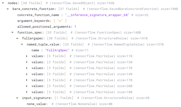
There are five protos that store definitions of function inputs in one manner or another. Their names and code locations, as well as their paths within the saved model proto, are as follows:

Proto messages, and their location in SavedModel

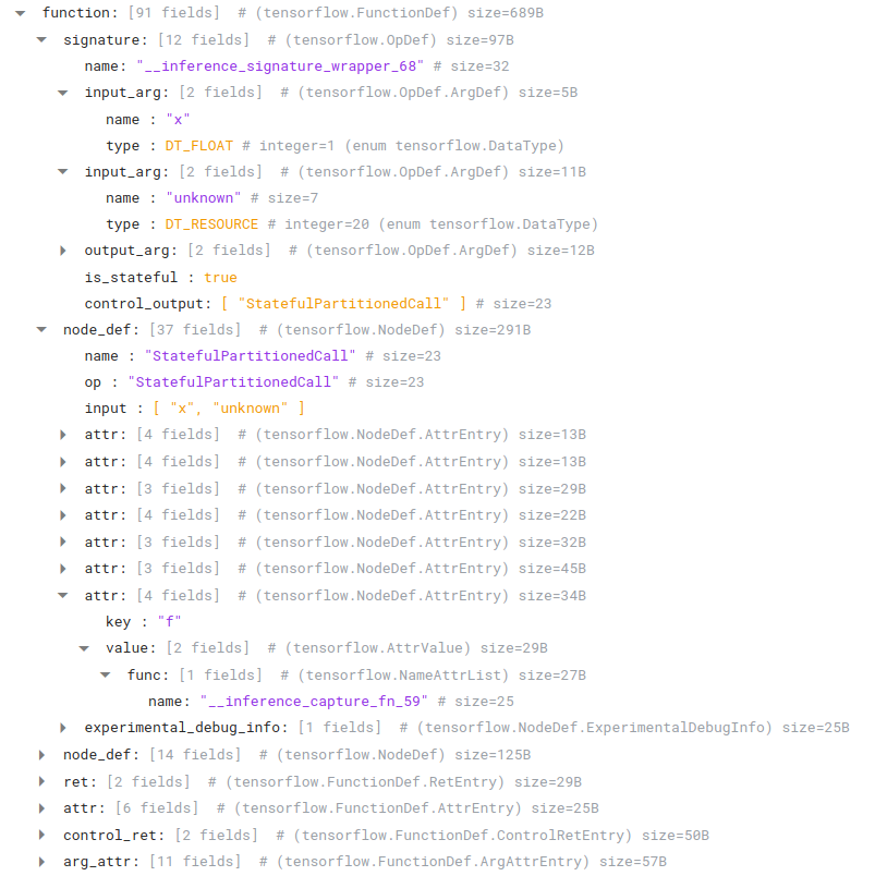
FunctionDef

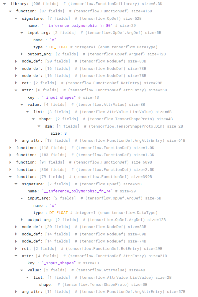
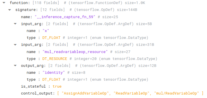
Of the five definitions discussed in this document, FunctionsDefs are the most core to execution. When loading a saved model, these function definitions are registered in the function library of the runtime and used to create ConcreteFunctions. These functions can then be executed via PartitionedCall or TFE_Py_Execute.

This is where the actual nodes describing execution are defined, as well as what the inputs and outputs to the function are.

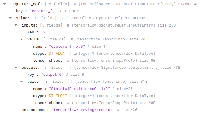
SignatureDef

SignatureDefs are generated from signatures passed into @tf.function. We do not save the signature’s TensorSpecs directly, however. Instead, when saving, we call the underlying function using the TensorSpecs in order to generate a concrete function. From there, we inspect the generated concrete function to get the inputs and outputs, storing them on the SignatureDef.

On the loading side,SignatureDefs are essentially ignored. They are primarily used in v1 or C++, where the developer loading the model can inspect the returned SignatureDef protos directly. This allows them to use their desired signature name to lookup the placeholder and output names needed for execution.

These input and output names can then be passed into feeds and fetches when calling Session.run in TensorFlow V1 code.

SavedFunction

SavedFunction is one of the many types of SavedObjects in the nodes list of the ObjectGraphDef. SavedFunctions are restored into a RestoredFunctions at load time. Like all nodes in this list, they are then attached to the returned model via the hierarchy defined by the children ObjectReference field.

SavedFunction’s main purpose is polymorphism. SavedFunctions support polymorphism by specifying a number of concrete function names defined in the function library above (via FunctionDef). At call time, we iterate through the concrete function names to find the first whose signature matches. If we find a match, we call it; if not, we throw an exception.

There is one more bit of complexity. When a RestoredFunction is called with a particular set of arguments, a new concrete function is created whose sole purpose is to call the matching concrete function. This is done using restored_function_body under the hood and is where the logic lives to find the appropriate concrete function.

This is invisible in the SavedModel proto, but these extra concrete functions are registered at call time in the runtime’s function library just as the other function library functions are.

The second purpose of SavedFunction is to update the FunctionSpec of all associated ConcreteFunctions using the FunctionSpec stored on the SavedFunction. This function spec is used at call time to

  1. validate passed in structured arguments, and
  2. convert structured arguments into flat ones needed for calling the underlying concrete function.

SavedBareConcreteFunction

Similar to SavedFunctions, SavedBareConcreteFunctions are used to update a

specific concrete function’s arguments and function spec. This is done here. Unlike SavedFunctions, they only reference a single specific concrete function.

In practice, SavedBareConcreteFunctions are commonly attached to and accessed via the signatures map (i.e. the signatures attribute on the loaded object). The underlying concrete functions they modify, in this case, are signature_wrapper functions. This wrapping is done to format the output in the way v1 expects (i.e. a dictionary of tensors). Similar to restored_function_body concrete functions, and other than restructuring the output, these concrete functions do nothing but call their associated concrete functions.

SavedConcreteFunction

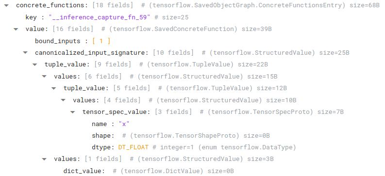
SavedConcreteFunction objects are not SavedObjectGraph nodes. They are stored in a map directly on the SavedObjectGraph. These objects reference a specific, already-registered concrete function — the key in the map is that concrete function’s registered name.

These objects serve two purposes. The first is handling function “captures” via

the bound_inputs field. Captured variables are those a function reads or modifies that were not explicitly passed in when calling into the function. Since functions in the function library do not have a concept of captured variables, any variables used by the function must be passed in as an argument. bound_inputs stores a list of node IDs that should be passed in to the underlying ConcreteFunction when called. We set this up here.

The second purpose, and similar to SavedFunction and SavedBareConcreteFunction, is modifying the existing concrete function’s FuncGraph structured inputs and outputs. This also is used for argument validation. The setup for this is done here.

Example Walkthrough

A simple example may help illustrate all of this with more clarity. Let’s make a basic model and take a look at the subsequent generated proto to get a better feel for what’s going on.

Basic Model

class ExampleModel(tf.Module):

@tf.function(input_signature=[tf.TensorSpec(shape=(), dtype=tf.float32)])
def capture_fn(self, x):
if not hasattr(self, 'weight'):
self.weight = tf.Variable(5.0, name='weight')
self.weight.assign_add(x * self.weight)
return self.weight

@tf.function
def polymorphic_fn(self, x):
return tf.constant(3.0) * x

model = ExampleModel()
model.polymorphic_fn(tf.constant(4.0))
model.polymorphic_fn(tf.constant([1.0, 2.0, 3.0]))
tf.saved_model.save(
model, "/tmp/example-model", signatures={'capture_fn': model.capture_fn})

This model contains the basis for most of the complexity we’ll need to fully explore the intricacies of saving and signatures. This will allow us to look at functions with and without signatures, with and without captures, and with and without polymorphism.

Function with Captures

Let’s start by looking at our function with captures, capture_fn. We can see we have a concrete function defined in the function library, as expected:

Image of concrete function defined in the function library
A FunctionDef located in FunctionDefLibrary of MetaGraphDef.graph_def

Note the expected float input, "x", as well as the additional captured argument, "mul_readvariableop_resource". Since this function has a capture, we should see a variable being referenced in the bound_inputs field of one of our SavedConcreteFunctions:

SavedConcreteFunctions
A SavedConcreteFunction located in the concrete_functions map of the ObjectGraphDef

Indeed, we can see bound_inputs refers to node 1, which is a SavedVariable with the name and dtype we expect:

A `SavedVariable` located in `ObjectGraphDef.nodes`
A SavedVariable located in ObjectGraphDef.nodes

Note that we also are storing on canonicalized_input_signature additional data that will be used to modify the concrete function. The key of this object, "__inference_capture_fn_59", is the same name as the concrete function registered in our function library.

Since we’ve specified a signature, we should also see a SavedBareConcreteFunction:

SavedBareConcreteFunction
A SavedBareConcreteFunction located in ObjectGraphDef.nodes

As discussed above, we use the function spec and argument information to modify the underlying concrete function. But what’s up with the "__inference_signature_wrapper_68" name? And how does this fit in with the rest of the code?

First, note that this is the fifth (5) node in the node list. This will come up again shortly.

Let’s start by looking at the nodes list. If we start at the first node in the nodes list, we’ll see a "signatures" node attached as a child:

SavedUserObject
A SavedUserObject located in ObjectGraphDef.nodes

If we look at node 2, we’ll see this node is a signature map that references one final node: node 5, our BareConcreteSavedFunction.

Node5
A SavedUserObject located in ObjectGraphDef.nodes

Thus, when we access this function via model.signatures["capture_fn"], we will actually be calling into this intermediate signature wrapper function first.

And what does that function, "__inference_signature_wrapper_68", look like?

FunctionDef
A FunctionDef located in FunctionDefLibrary of MetaGraphDef.graph_def

It takes the arguments we expect, and makes a call out to… "__inference_capture_fn_59", our original function! Just as we expect.

But wait… what happens if we don’t access our function via model.signatures["capture_fn"]? After all, we should be able to call it directly via model.capture_fn.

Notice above, we had a child on the top level object named "capture_fn" with a node_id of 3. If we look at node 3, we’ll see a SavedFunction object that references our original concrete function with no signature wrapper intermediary:

Node 3
A SavedFunction located in ObjectGraphDef.nodes

Again, the function spec is used to modify the function spec of our concrete function, "__inference_capture_fn_59". Notice also that concrete_functions here is a list. We only have one item right now, but this will come up again when we take a look at our polymorphic function example.

Now, we’ve fully mapped essentially everything needed for execution of this function, but we have one last thing to look at: SignatureDef. We’ve defined a signature, so we expect a SignatureDef to be defined:

SignatureDef
A SignatureDef located in the MetaObjectGraph.signature_def map

This is very important for loading in v1 and C++ for serving. Note those funky names: "capture_fn_x:0" and "StatefulPartitionedCall:0". To call this function in v1, we need a way to map our nice argument names to the actual graph placeholder names for passing in as feeds and fetches (and doing validation, if we wish). Looking at this SignatureDef allows us to do just that.

Polymorphic Functions

We’re not quite done yet. Let’s take a look at our polymorphic function. We won’t repeat everything, since a lot of it is the same. We won’t have any signature wrapper functions or signature defs, since we skipped the signature on this one. Let’s look at what’s different.

A Polymorphic FunctionDef
A FunctionDef located in FunctionDefLibrary of MetaGraphDef.graph_def

For one, we now have two concrete functions registered in the function library, each with slightly different input shapes.

We also have two SavedConcreteFunction modifiers:

Two SavedConcreteFunctions
Two SavedConcreteFunctions located in the concrete_functions map of the ObjectGraphDef

And finally, we can see our SavedFunction references two underlying concrete functions instead of one:

SavedFunction
A SavedFunction located in ObjectGraphDef.nodes

The function spec here will be attached to both of these concrete functions at load time. When we call our SavedFunction, it will use the arguments we pass in to find the correct concrete function and execute it.

Next Steps

You should now be an expert on how functions and their signatures are saved at a code level. Remember, what’s described in this blog post is how the code works right now. For updated code and examples in the future, see the official documentation on tensorflow.org.

Speaking of documentation, if you want a fast introduction to the basic APIs for saved models, you should introductory articles on how the APIs for functions and modules are traced and saved. For experts, don’t miss this detailed guide on SavedModel itself, as well as a complete discussion of autograph.

And finally, if you do any exciting or useful protobuf surgery, share with us on Twitter. Thanks for reading this far!

Read More