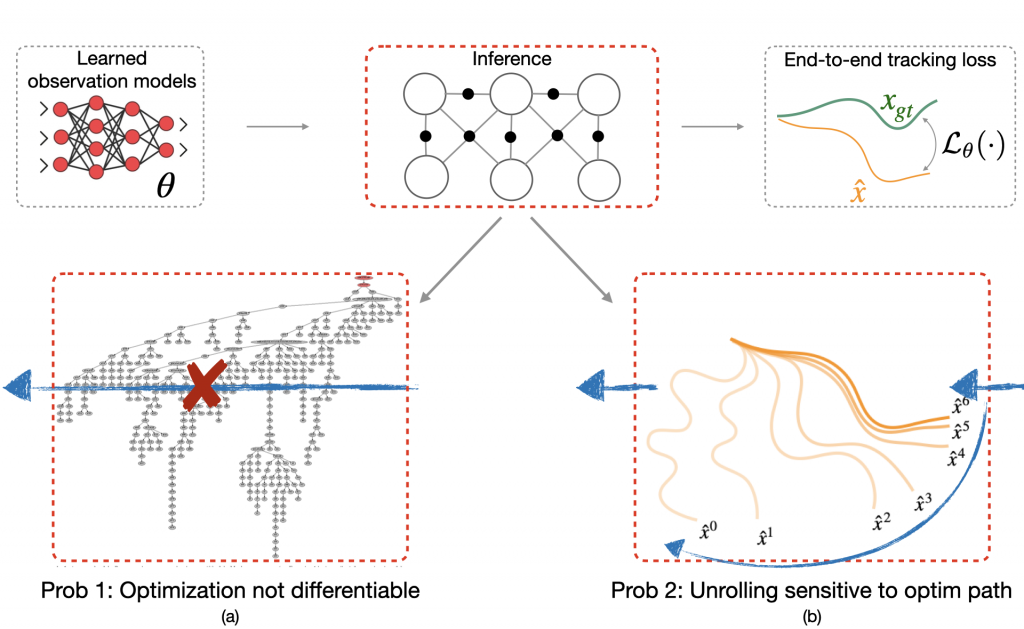
Fig. 1 We show that learning observation models can be viewed as shaping energy functions that graph optimizers, even non-differentiable ones, optimize. Inference solves for most likely states (x) given model and input measurements (z.) Learning uses training data to update observation model parameters (theta).
Robots perceive the rich world around them through the lens of their sensors. Each sensor observation is a tiny window into the world that provides only a partial, simplified view of reality. To complete their tasks, robots combine multiple readings from sensors into an internal task-specific representation of the world that we call state. This internal picture of the world enables robots to evaluate the consequences of possible actions and eventually achieve their goals. Thus, for successful operations, it is extremely important to map sensor readings into states in an efficient and accurate manner.
Conventionally, the mapping from sensor readings to states relies on models handcrafted by human designers. However, as sensors become more sophisticated and capture novel modalities, constructing such models becomes increasingly difficult. Instead, a more scalable way forward is to convert sensors to tensors and use the power of machine learning to translate sensor readings into efficient representations. This brings up the key question of this post: What is the learning objective? In our recent CoRL paper, LEO: Learning Energy-based Models in Factor Graph Optimization, we propose a conceptually novel approach to mapping sensor readings into states. In that, we learn observation models from data and argue that learning must be done with optimization in the loop.
How does a robot infer states from observations?
Consider a robot hand manipulating an occluded object with only tactile image feedback. The robot never directly sees the object: all it sees is a sequence of tactile images (Lambeta 2020, Yuan 2017). Take a look at any one such image (Fig. 2). Can you tell what the object is and where it might be just from looking at a single image? It seems difficult, right? This is why robots need to fuse information collected from multiple images.
Fig. 2 A robot hand receives a sequence of tactile image observations from which it must infer a sequence of latent object poses. We formulate this as an inference over a factor graph that in turn relies on a mapping between observations and states provided by an observation model.
How do we fuse information from multiple observations? A powerful way to do this is by using a factor graph (Dellaert 2017). This approach maintains and dynamically updates a graph where variablenodes are the latent states and edges or factor nodes encode measurements as constraints between variables. Inference solves for the objective of finding the most likely sequence of states given a sequence of observations. Solving for this objective boils down to an optimization problem that can be computed efficiently in an online fashion.
Factor graphs rely on the user specifying an observation model that encodes how likely an observation is given a set of states. The observation model defines the cost landscape that the graph optimizer minimizes. However, in many domains, sensors that produce observations are complex and difficult to model. Instead, we would like to learn the observation model directly from data.
Can we learn observation models from data?
Let’s say we have a dataset of pairs of ground truth state trajectories (x_{gt}) and observations (z). Consider an observation model with learnable parameters (theta) that maps states and observations to a cost. This cost is then minimized by the graph optimizer to get a trajectory (hat{x}). Our objective is to minimize the end-to-end loss (L_{theta}(hat{x},x_{gt})) between the optimized trajectory (hat{x}) and the ground truth (x_{gt}).
What would a typical learning procedure look like? In the forward pass, we have a learned observation model feeding into the graph optimizer to produce an optimized trajectory (hat{x}) (Fig. 3). This is then compared to a ground truth trajectory (x_{gt}) to compute the loss (L_{theta}(.)). The loss is then back-propagated through the inference step to update (theta).
Fig. 3 Two problems arise when directly back-propagating through the optimizer. (a) Many state-of-the-art graph optimizers are not natively differentiable (b) Differentiation via unrolling sensitive to the optimization procedure used during training.
However, there are two problems with this approach. The first problem is that many state-of-the-art optimizers are not natively differentiable. For instance, the iSAM2 graph optimizer (Kaess 2012) used popularly for simultaneous localization and mapping (SLAM) invokes a series of non-differentiable Bayes tree operations and heuristics (Fig. 3a). Secondly, even if one did want to differentiate through the nonlinear optimizer, one would typically do this by unrolling successive optimization steps, and then propagating back gradients through the optimization procedure (Fig. 3b). However, training in this manner can have undesired effects. For example, prior work (Amos 2020) shows instances where even though unrolling gradient descent drives training loss to 0, the resulting cost landscape does not have a minimum on the ground truth. In other words, the learned cost landscape is sensitive to the optimization procedure used during training, e.g., the number of unrolling steps or learning rate.
Learning an energy landscape for the optimizer
We argue that instead of worrying about the optimization procedure, we should only care about the landscape of the energy or cost function that the optimizer has to minimize. We would like to learn an observation model that creates an energy landscape with a global minimum on the ground truth. This is precisely what energy-based models aim to do (LeCun 2006) and that is what we propose in our novel approach LEO that applies ideas from energy-based learning to our problem.
How does LEO work? Let us now demonstrate the inner workings of our approach on a toy example. For this, let us consider a one-dimensional visualization of the energy function represented in Fig 4. We collapse the trajectories down to a single axis. LEO begins by initializing with a random energy function. Note that the ground truth (x_{gt}) is far from the minimum. LEO samples trajectories (hat{x}) around the minimum by invoking the graph optimizer. It then compares these against ground truth trajectories and updates the energy function. The energy-based update rule is simple — push down the cost of ground truth trajectories (x_{gt}) and push up the cost of samples (hat{x}), with the cost of samples effectively acting as a contrastive term. If we keep iterating on this process, the minimum of the energy function eventually centers around the ground truth. At convergence, the gradients of the samples (hat{x}) on average match the gradient of the ground truth trajectory (x_{gt}). Since the samples are over a continuous space of trajectories for which exact computation of the log partition function is intractable, we propose a way to generate such samples efficiently using an incremental Gauss-Newton approximation (Kaess 2012).
Fig. 4 Let’s initialize with a random energy function shown in blue. LEO begins by sampling trajectories (hat{x}) around the minimum by invoking the graph optimizer. It then compares these against ground truth trajectories and updates the energy function. The energy-based update rule is simple — push down the cost of ground truth trajectories and push up samples around the minimum. Upon repeating this process, the minimum of this function eventually centers around the ground truth. At convergence, gradients of samples (hat{x}) on average match gradient of the ground truth trajectory (x_{gt}).
How does LEO perform in practice? Let’s being with a simple regression problem (Amos 2020). We have pairs of ((x,y)) from a ground truth function (y=xsin(x)) and we would like to learn an energy function (E_theta(x,y)) such that (y = {operatorname{argmin}}_{y’} E_theta(x,y’)). LEO begins with a random energy function, but after a few iterations, learns an energy function with a distinct minimum around the ground truth function shown in solid line (Fig. 5). Contrast this to the energy functions learned by unrolling. Not only does it not have a distinct minimum around the ground truth, but it also varies with parameters like the number of unrolling iterations. This is because the learned energy landscape is specific to the optimization procedure used during learning.
Fig. 5 Visualize learned energy landscapes on a 1D regression problem. The goal is to learn a network that maps points (x,y) to an energy value (E_theta(x,y)) given samples from a ground truth function (y=xsin(x)) shown in solid line. LEO learns an energy landscape (E_theta(.)) with a distinct minimum (in white) around ground truth. In contrast, the energy landscape learned via unrolling does not have a distinct minimum (in white) and varies with optimization parameters during training.
Application to Robotics Problems
We evaluate LEO on two distinct robot applications, comparing it to baselines that either learn sequence-to-sequence networks or black-box search methods.
The first is a synthetic navigation task where the goal is to estimate robot poses from odometry and GPS observations. Here we are learning covariances, e.g., how noisy is GPS compared to odometry. Even though LEO is initialized far from the ground truth, it is able to learn parameters that pull the optimized trajectories close to the ground truth (Fig. 6).
Fig. 6Synthetic navigation application. LEO learns covariance parameters every iteration to drive optimized trajectories close to ground truth.
We also look at a real-world manipulation task where an end-effector equipped with a touch sensor is pushing an object (Sodhi 2021). Here we learn a tactile model that maps a pair of tactile images to relative poses used in conjunction with physics and geometric priors. We show that LEO is able to learn parameters that pull optimized trajectories close to the ground truth or various object shapes and pushing trajectories (Fig. 7).
Fig. 7Real-world planar pushing application. LEO learns model parameters every iteration to drive optimized trajectories close to ground truth.
Parting Thoughts
While we focused on learning observation models for perception, the insights on learning energy landscapes for an optimizer extend to other domains such as control and planning. An increasingly unified view of robot perception and control is that both are fundamentally optimization problems. For perception, the objective is to optimize a sequence of states that explain the observations. For control, the objective is to optimize a sequence of actions that accomplish a task.
But what should the objective function be for both of these optimizations? Instead of hand designing observation models for perception or hand designing cost functions for control, we should leverage machine learning to learn these functions from data. To do so easily at scale, it is imperative that we build robotics pipelines and datasets that facilitate learning with optimizers in the loop.
[1] Dellaert and Kaess. Factor graphs for robot perception. Foundations and Trends in Robotics, 2017. [2] Kaess et al. iSAM2: Incremental smoothing and mapping using the Bayes tree. Intl. J. of Robotics Research (IJRR), 2012. [3] LeCun et al. A tutorial on energy-based learning. Predicting structured data, 2006. [4] Ziebart et al. Maximum entropy inverse reinforcement learning. AAAI Conf. on Artificial Intelligence, 2008. [5] Amos and Yarats. The differentiable cross-entropy method. International Conference on Machine Learning (ICML), 2020. [6] Yi et al. Differentiable factor graph optimization for learning smoothers. IEEE/RSJ Intl. Conf. on Intelligent Robots and Systems (IROS), 2021. [7] Sodhi et al. Learning tactile models for factor graph-based estimation. IEEE Intl. Conf. on Robotics and Automation (ICRA), 2021. [8] Lambeta et al. DIGIT: A novel design for a low-cost compact high-resolution tactile sensor with application to in-hand manipulation. IEEE Robotics and Automation Letters (RAL), 2020.
The Benefits of Machines that Understand User Interfaces
Machines that understand and operate user interfaces (UIs) on behalf of users could offer many benefits. For example, a screen reader (e.g., VoiceOver and TalkBack) could facilitate access to UIs for blind and visually impaired users, and task automation agents (e.g., Siri Shortcuts and IFTTT) could allow users to automate repetitive or complex tasks with their devices more efficiently. These benefits are gated on how well these systems can understand an underlying app’s UI by reasoning about 1) the functionality present, 2) how its different components work together, and 3) how it can be operated to accomplish some goal. Many rely on the availability of UI metadata (e.g., the view hierarchy and the accessibility hierarchy), which provide some information about what elements are present and their properties. However, this metadata is often unavailable due to poor toolkit support and low developer awareness. To maximize their support of apps and when they are helpful to users, these systems can benefit from understanding UIs solely from visual appearance.
Recent efforts have focused on predicting the presence of an app’s on-screen elements and semantic regions solely from its visual appearance. These have enabled many useful applications: such as allowing assistive technology to work with inaccessible apps and example-based search for UI designers. However, they constitute only a surface-level understanding of UIs, as they primarily focus on extracting what elements are on a screen and where they appear spatially. To further advance the UI understanding capabilities of machines and perform more valuable tasks, we focus on modeling the higher-level relationships by predicting UI structure.
Our work makes the following contributions:
A problem defnition of screen parsing which is useful for a wide range of UI modeling applications
A description of our implementation and its training procedure
A comprehensive evaluation of our implementation with baseline comparison
Three implemented examples of how our model can be used to facilitate downstream applications such as (i) UI similarity, (ii) accessibility metadata generation, and (iii) code generation.
Achieving Better Understanding of UIs through Hierarchy
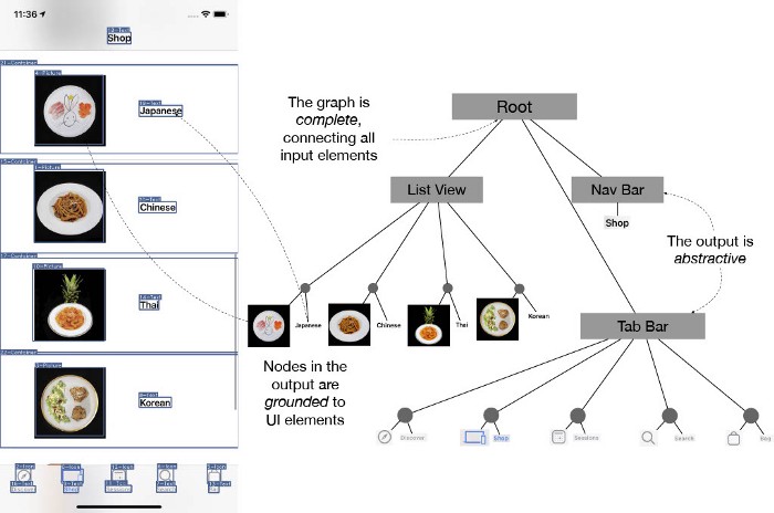
An example of an input screen (Left) and the corresponding UI Hierarchy (Right). The tree contains all of the visible elements on the screen (the output is complete), groups them together to form higher-level structures (abstractive), and nodes can be used to reference UI elements (the output is grounded)
Structural representations enhance the understanding of many types of content by capturing higher-level semantics. For example, scene graphs enrich visual scenes by making sense of interactions between individual objects and parse trees disambiguate sentences by analyzing their grammar. Similarly, structure is a core property of UIs reflected in how they are constructed (i.e., stacking together views and widgets) and used. Modeling element relationships can help machines perceive UIs as humans do — not as a set of elements but as a coordinated presentation of content.
We introduce the problem of screen parsing, which we use to predict structured UI models (a high-level definition of a UI) from visual information. We focus on generating an app screen’s UI hierarchy, which specifies how UI elements are grouped and rendered on the screen. The following are properties of UI hierarchies:
Complete — the output is a single directed tree that spans all of the UI elements on a screen
Grounded — nodes in the output reference on-screen elements and regions
Abstractive — the output can group elements (potentially more than once) to form higher-level structures.
Predicting UI Hierarchy from a Screenshot
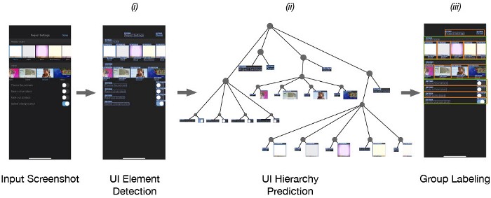
An overview of our implementation of screen parsing. To infer the structure of an app screen, our system (i) detects the location and type of UI elements from a screenshot, (ii) predicts a graph structure that describes the relationships between UI elements, and (iii) classifies groups of UI elements.
To predict UI hierarchy from a screenshot, we built a system to:
detect the location and type of UI elements from a screenshot,
predict a hierarchical structure that describes the relationships between them, and
classify semantic groups.
The first step of our system processes a screenshot image using an object detection model (Faster-RCNN), which produces a list of UI element detections. The output is post-processed using standard techniques such as confidence-thresholding and non-max suppression. This list tells us what elements are on the screen and where they are but does not provide any information about their relationship.
Next, we use a stack-pointer parsing model to generate a tree structure representing UI hierarchy. Like other transition-based parsers, our model incrementally predicts a tree structure by generating a sequence of actions that build connections between UI elements using a pointer mechanism. We made two modifications to the original stack-pointer dependency parsing to adapt the parsing model for UI hierarchies. First, we injected a “container” token into the input, allowing the model to create multi-level groupings. Second, we trained the model using a dynamic oracle to reduce exposure bias since the multi-level nature of UI hierarchies leads to exponentially more “optimal” action sequences that produce the same output.
To illustrate how our model predicts UI hierarchy, we will describe the inference process. A flat list of detected UI elements is encoded using a bi-directional LSTM encoder (producing a list l of encoded elements), and the final hidden state is fed to an LSTM decoder network augmented with two data structures: 1) a stack (s) which is used by the network as intermediate memory and 2) a set (v) which records the set of nodes already processed. The stack s is initialized with a special node that represents the root of the tree. At each timestep, the element on top of s and the last hidden state is fed into the decoder network, which outputs one of three actions:
Arc – A directed edge is created between the node on top of s (parent) and the node in l – v with the highest attention score (child). The child is pushed on s and added to v. This action attaches one of the detected UI elements onto the tree.
Emit – An intermediate node (represented as a zero-vector) is created and pushed onto s. This action helps the model represent container or “grouping” elements, such as lists, that do not exist in l.
Pop – s is popped. This occurs when the model has finished adding all of an element’s children to the tree structure.
This technique for generating parse trees is widely used in NLP, and it has been shown that a correct sequence of actions exists for any target tree. Note that this was originally shown for a limited subset of parse trees known as “projective” parse trees, but recent work has extended it to handle any type of tree.
Finally, we apply a set classification model to label containers (i.e., intermediate nodes) based on their descendants. We defined seven container types (including an “Other” class) that represent common groupings such as collections (e.g., lists, grids), tables, and tab bars.
Screen Parser uses a multi-step process to infer the UI hierarchy from a screenshot. Element detections are iteratively grouped together using a parsing model that produces a sequence of special actions called transitions (transition-based parsing).
We trained our models on two mobile UI datasets: (i) AMP dataset of ~130,000 iOS screens, and (ii) RICO, a publicly available dataset of ~80,000 Android screens. Both datasets were collected by crowdworkers who installed and explored popular apps across 20+ categories (in some cases excluding certain ones such as games, AR, and multimedia) on the iOS and Android app stores. Each dataset contains screenshots, annotated screens, and a type of metadata called a view hierarchy. The view hierarchy is an artifact generated during UI rendering that describes which interface widgets are used and “stacked” together to produce the final layout. Not all screens in our dataset contain this metadata, especially apps created using third-party UI toolkits or game engines. We apply heuristics to detect and exclude examples with missing or incomplete view hierarchies. The view hierarchies are similar to the presentation model we aim to predict, with a few differences, so we transform them into our target representation by applying graph smoothing, filtering, and element matching between different data sources.
More details about our machine learning models and training procedures can be found in our paper.
Experiments
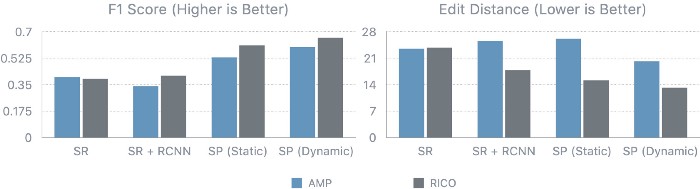
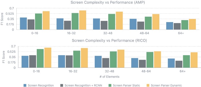
We used several metrics (e.g., F1 score, graph edit distance) to perform a quantitative evaluation of our system using the test split of our mobile UI datasets. Our main point of comparison was a heuristic-based approach to inferring screen groupings used in previous work, and we found that our system was much more accurate in inferring UI hierarchy. We also found that our improved training procedure led to significant performance gains (23%) over standard methods for training parsers.
Our system’s performance is affected by a number of factors such as screen complexity and object detection errors. Accuracy is highest for screens up to 32 elements and degrades following that point, in part due to the increased number of actions the parsing model must correctly predict. Complex and crowded screens introduce the additional difficulty of detecting small UI elements, which our analysis with a matching-based oracle (computes best possible matching between object detection output and ground truth) shows as a limiting factor.
UI Hierarchy Facilitates and Improves Applications
We present a suite of example applications implemented using our screen parsing system. These applications show the versatility of our approach and how the predicted UI hierarchy facilitates many downstream tasks.
UI Similarity
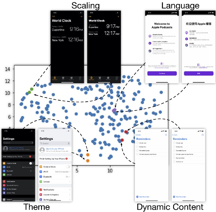
We used our system to generate embedding vectors for different UI screens that capture their structure, instead of their surface-level appearance. We show that embeddings for the same screen are minimally affected by different display settings (e.g., scaling, language, theme, dynamic content).
Many recent efforts in modeling UIs have focused on representing them as fixed-length embedding vectors. These vectors can be trained to encode different properties of UI screens, such as layout, content, and style, and they can be fine-tuned to support downstream tasks. For example, a common application of embedding models is measuring screen similarity, which is represented by distance in embedding space. We believe the performance of such models can be improved by incorporating structural information, an important property of UIs.
The intermediate representation of our parsing model can be used to produce a screen embedding, which describes the hierarchical structure of an app. To generate an embedding of a UI, we feed it into our model and pool the last hidden state of the encoder. This includes information about the position, type, and structure of on-screen elements. Our structural embedding can help minimize variations from display settings such as (i) scaling, (ii) language, (iii) theme, and (iv) small dynamic changes. The properties of our embedding could be useful for some UI understanding applications, such as app crawling and information extraction where it would be beneficial to disentangle screen structure and appearance. For example, an app crawler’s next action should be conditioned on the UI elements present on the screen, not on the user’s current theme. An autoencoder trained on UI screenshots would not have this property.
Accessibility Improvement
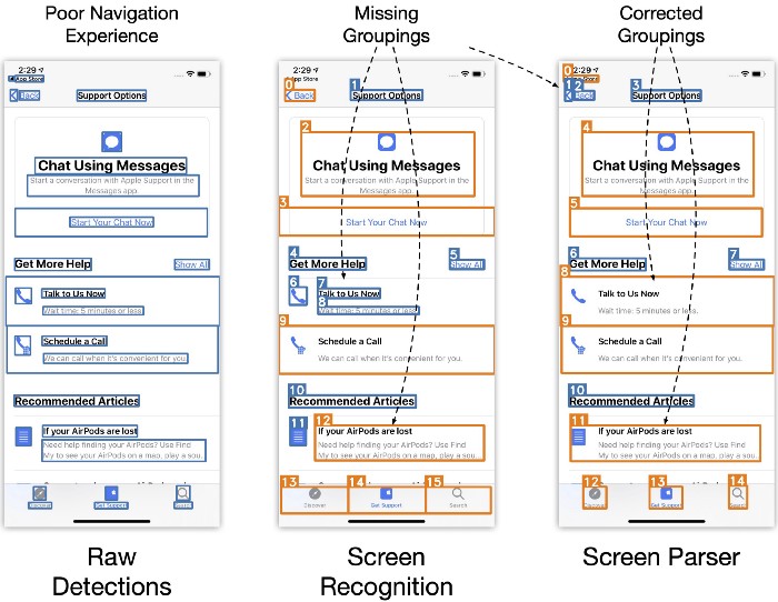
Element boxes are annotated using their navigation ordering, where the number represents how many swipes are needed to access the element when using a screen reader. While both results contain errors, in this case, Screen Parser correctly groups more elements, which decreases the number of swipes needed to access elements.
Recent work has successfully generated missing metadata for inaccessible apps by running an object detection model on the UI screenshot. Their approach to generating hierarchical data relies on manually defined heuristics that detect localized patterns between elements. However, these approaches may sometimes fail because they do not have access to global information necessary for resolving ambiguities.
In contrast, our implementation generates a UI hierarchy with a global view of the input, so it can overcome some of the limitations of heuristic-based approaches. We used the predicted UI hierarchy to group together the children of intermediate nodes of height 1 that contained at most one text label and used the X-Y cut algorithm to determine navigation order. The figure above shows an example where the grouping output from the Screen Parsing model is more accurate than the one produced by manually-defined. While this is not always the case, learning grouping rules from data requires much less human effort than manual heuristic engineering.
Code Generation
By mapping nodes in the UI hierarchy to declarative view-creation methods, we can generate code for a UI from its screenshot. Here, a restaurant app is re-rendered on a tablet form-factor.
Existing approaches to code generation also rely on heuristics to detect a limited subset of container types. We employed a technique used by compilers to generate code from abstract syntax trees (AST) (the visitor pattern for code generation) and applied it to the predicted UI hierarchy. Specifically, we performed a depth-first traversal of the UI hierarchy using a visitor function that generates code based on the current state (current node and stack). The visitor function emits a SwiftUI control (e.g., Text, Toggle, Button) at every leaf node and emits a SwiftUI container (e.g., VStack, HStack) at every intermediate node. Additional parameters required by view constructors, such as label text and background color were extracted using OCR and a small set of heuristics.
The resulting code describes the original UI using only relative constraints (even if the original UI was not), allowing it to act responsively to changes in screen size or device type. The generated code does not contain appearance and style information, which is sometimes necessary to render a similar-looking screen. Nevertheless, prior work has shown that such output can be a useful starting point for UI development, and we believe future work can improve upon our approach by detecting these properties.
Conclusion
To help machines better reason about the underlying structure and purpose of UIs, we introduced the problem of screen parsing, the prediction of structured UI models from visual information. Our problem formulation captures the structural properties of UIs and is well-suited for downstream applications that rely on UI understanding. We described the architecture and training procedure for our reference implementation, which predicts an app’s presentation model as a UI hierarchy with high accuracy, surpassing baseline algorithms and training procedures. Finally, we used our system to build three example applications: (i) UI similarity search, (ii) accessibility enhancement, and (iii) code generation from UI screenshots. Screen parsing is an important step towards full machine understanding of UIs and its many benefits, but there is still much left to do. We’re excited by the opportunities at the intersection of HCI and ML, and we encourage other researchers in the ML community to work with us to realize this goal.
Acknowledgements
Many people contributed to this work and gave feedback on this blog post: Xiaoyi Zhang, Jeff Nichols, and Jeff Bigham. This work was done while Jason Wu was an intern at Apple.
Jason Wu, Xiaoyi Zhang, Jeffrey Nichols, and Jeffrey P. Bigham. 2021. Screen Parsing: Towards Reverse Engineering of UI Models from Screenshots. In Proceedings of the 2021 ACM Symposium on User Interface Software & Technology (UIST). Association for Computing Machinery, New York, NY, USA, 1–10. https://doi.org/10.1145/3472749.3474763
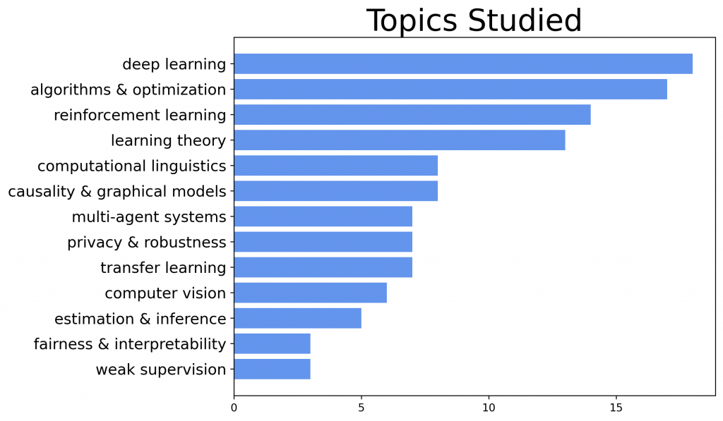
Carnegie Mellon University is proud to present 92 papers in the main conference and 9 papers in the datasets and benchmarks track at the 35th Conference on Neural Information Processing Systems (NeurIPS 2021), which will be held virtually this week. Additionally, CMU faculty and students are co-organizing 6 workshops and 1 tutorial, as well as giving 7 invited talks at the main conference and workshops. Here is a quick overview of the areas our researchers are working on:
Topics of CMU papers at NeurIPS 2021 (each paper may be assigned multiple topics).
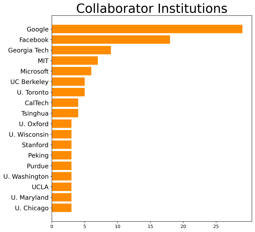
We are also proud to collaborate with many other researchers in academia and industry:
Institutions with at least three external collaborators on CMU papers at NeurIPS 2021.
Conference Papers
Algorithms & Optimization
Adversarial Robustness of Streaming Algorithms through Importance Sampling Vladimir Braverman (Johns Hopkins University) · Avinatan Hassidim (Google) · Yossi Matias (Tel Aviv University) · Mariano Schain (Google) · Sandeep Silwal (Massachusetts Institute of Technology) · Samson Zhou (Carnegie Mellon University) Tue Dec 07 08:30 AM — 10:00 AM (PST) @ Poster Session 1 Spot G1
On Large-Cohort Training for Federated Learning Zachary Charles (Google Research) · Zachary Garrett (Google) · Zhouyuan Huo (Google) · Sergei Shmulyian (Google) · Virginia Smith (Carnegie Mellon University) Thu Dec 09 08:30 AM — 10:00 AM (PST) @ Poster Session 6 Spot D1
Federated Reconstruction: Partially Local Federated Learning Karan Singhal (Google Research) · Hakim Sidahmed (Carnegie Mellon University) · Zachary Garrett (Google) · Shanshan Wu (University of Texas at Austin) · Keith Rush (Google) · Sushant Prakash (Google) Thu Dec 09 08:30 AM — 10:00 AM (PST) @ Poster Session 6 Spot C0
Habitat 2.0: Training Home Assistants to Rearrange their Habitat Andrew Szot (Georgia Institute of Technology) · Alexander Clegg (Facebook (FAIR Labs)) · Eric Undersander (Facebook) · Erik Wijmans (Georgia Institute of Technology) · Yili Zhao (Facebook AI Research) · John Turner (Facebook) · Noah Maestre (Facebook) · Mustafa Mukadam (Facebook AI Research) · Devendra Singh Chaplot (Carnegie Mellon University) · Oleksandr Maksymets (Facebook AI Research) · Aaron Gokaslan (Facebook) · Vladimír Vondruš (Magnum Engine) · Sameer Dharur (Georgia Tech) · Franziska Meier (Facebook AI Research) · Wojciech Galuba (Facebook AI Research) · Angel Chang (Simon Fraser University) · Zsolt Kira (Georgia Institute of Techology) · Vladlen Koltun (Apple) · Jitendra Malik (UC Berkeley) · Manolis Savva (Simon Fraser University) · Dhruv Batra () Thu Dec 09 12:30 AM — 02:00 AM (PST) @ Poster Session 5 Spot E0
Joint inference and input optimization in equilibrium networks Swaminathan Gurumurthy (Carnegie Mellon University) · Shaojie Bai (Carnegie Mellon University) · Zachary Manchester (Carnegie Mellon University) · J. Zico Kolter (Carnegie Mellon University / Bosch Center for A) Thu Dec 09 04:30 PM — 06:00 PM (PST) @ Poster Session 7 Spot E1
On Training Implicit Models Zhengyang Geng (Peking University) · Xin-Yu Zhang (TuSimple) · Shaojie Bai (Carnegie Mellon University) · Yisen Wang (Peking University) · Zhouchen Lin (Peking University) Fri Dec 10 08:30 AM — 10:00 AM (PST) @ Poster Session 8 Spot G2
Robust Online Correlation Clustering Silvio Lattanzi (Google Research) · Benjamin Moseley (Carnegie Mellon University) · Sergei Vassilvitskii (Google) · Yuyan Wang (Carnegie Mellon University) · Rudy Zhou (CMU, Carnegie Mellon University) Fri Dec 10 08:30 AM — 10:00 AM (PST) @ Poster Session 8 Spot A1
Instance-dependent Label-noise Learning under a Structural Causal Model Nick Yao (University of Sydney) · Tongliang Liu (The University of Sydney) · Mingming Gong (University of Melbourne) · Bo Han (HKBU / RIKEN) · Gang Niu (RIKEN) · Kun Zhang (CMU) Tue Dec 07 08:30 AM — 10:00 AM (PST) @ Poster Session 1 Spot G3
Multi-task Learning of Order-Consistent Causal Graphs Xinshi Chen (Georgia Institution of Technology) · Haoran Sun (Georgia Institute of Technology) · Caleb Ellington (Carnegie Mellon University) · Eric Xing (Petuum Inc. / Carnegie Mellon University) · Le Song (Georgia Institute of Technology) Wed Dec 08 04:30 PM — 06:00 PM (PST) @ Poster Session 4 Spot C3
Learning latent causal graphs via mixture oracles Bohdan Kivva (University of Chicago) · Goutham Rajendran (University of Chicago) · Pradeep Ravikumar (Carnegie Mellon University) · Bryon Aragam (University of Chicago) Fri Dec 10 08:30 AM — 10:00 AM (PST) @ Poster Session 8 Spot C0
Computational Linguistics
BARTScore: Evaluating Generated Text as Text Generation Weizhe Yuan (Carnegie Mellon University) · Graham Neubig (Carnegie Mellon University) · Pengfei Liu (Carnegie Mellon University) Tue Dec 07 08:30 AM — 10:00 AM (PST) @ Poster Session 1 Spot A3
Off-Policy Risk Assessment in Contextual Bandits Audrey Huang (Carnegie Mellon University) · Liu Leqi (Carnegie Mellon University) · Zachary Lipton (Carnegie Mellon University) · Kamyar Azizzadenesheli (Purdue University) Tue Dec 07 08:30 AM — 10:00 AM (PST) @ Poster Session 1 Spot C2
SegFormer: Simple and Efficient Design for Semantic Segmentation with Transformers Enze Xie (The University of Hong Kong) · Wenhai Wang (Nanjing University) · Zhiding Yu (Carnegie Mellon University) · Anima Anandkumar (NVIDIA / Caltech) · Jose M. Alvarez (NVIDIA) · Ping Luo (The University of Hong Kong) Tue Dec 07 08:30 AM — 10:00 AM (PST) @ Poster Session 1 Spot A3
(Implicit)^2: Implicit Layers for Implicit Representations Zhichun Huang (CMU, Carnegie Mellon University) · Shaojie Bai (Carnegie Mellon University) · J. Zico Kolter (Carnegie Mellon University / Bosch Center for A) Thu Dec 09 08:30 AM — 10:00 AM (PST) @ Poster Session 6 Spot D1
Foundations of Symbolic Languages for Model Interpretability Marcelo Arenas (Pontificia Universidad Catolica de Chile) · Daniel Báez (Universidad de Chile) · Pablo Barceló (PUC Chile & Millenium Instititute for Foundational Research on Data) · Jorge Pérez (Universidad de Chile) · Bernardo Subercaseaux (Carnegie Mellon University) Fri Dec 10 08:30 AM — 10:00 AM (PST) @ Poster Session 8 Spot C1
Keeping Your Eye on the Ball: Trajectory Attention in Video Transformers Mandela Patrick (University of Oxford) · Dylan Campbell (University of Oxford) · Yuki Asano (University of Amsterdam) · Ishan Misra (Facebook AI Research) · Florian Metze (Carnegie Mellon University) · Christoph Feichtenhofer (Facebook AI Research) · Andrea Vedaldi (University of Oxford / Facebook AI Research) · João Henriques (University of Oxford) Fri Dec 10 08:30 AM — 10:00 AM (PST) @ Poster Session 8 Spot C3
Computer Vision
Dynamics-regulated kinematic policy for egocentric pose estimation Zhengyi Luo (Carnegie Mellon University) · Ryo Hachiuma (Keio University) · Ye Yuan (Carnegie Mellon University) · Kris Kitani (Carnegie Mellon University) Tue Dec 07 08:30 AM — 10:00 AM (PST) @ Poster Session 1 Spot D3
NeRS: Neural Reflectance Surfaces for Sparse-view 3D Reconstruction in the Wild Jason Zhang (Carnegie Mellon University) · Gengshan Yang (Carnegie Mellon University) · Shubham Tulsiani (UC Berkeley) · Deva Ramanan (Carnegie Mellon University) Tue Dec 07 08:30 AM — 10:00 AM (PST) @ Virtual @ Poster Session 1 Spot D0
SEAL: Self-supervised Embodied Active Learning using Exploration and 3D Consistency Devendra Singh Chaplot (Carnegie Mellon University) · Murtaza Dalal (Carnegie Mellon University) · Saurabh Gupta (UIUC) · Jitendra Malik (UC Berkeley) · Russ Salakhutdinov (Carnegie Mellon University) Wed Dec 08 04:30 PM — 06:00 PM (PST) @ Poster Session 4 Spot A1
TöRF: Time-of-Flight Radiance Fields for Dynamic Scene View Synthesis battal Attal (Carnegie Mellon University) · Eliot Laidlaw (Brown University) · Aaron Gokaslan (Facebook) · Changil Kim (Facebook) · Christian Richardt (University of Bath) · James Tompkin (Brown University) · Matthew O’Toole (Carnegie Mellon University) Thu Dec 09 04:30 PM — 06:00 PM (PST) @ Poster Session 7 Spot E3
ViSER: Video-Specific Surface Embeddings for Articulated 3D Shape Reconstruction Gengshan Yang (Carnegie Mellon University) · Deqing Sun (Google) · Varun Jampani (Google) · Daniel Vlasic (Massachusetts Institute of Technology) · Forrester Cole (Google Research) · Ce Liu (Microsoft) · Deva Ramanan (Carnegie Mellon University) Thu Dec 09 08:30 AM — 10:00 AM (PST) @ Poster Session 6 Spot A2
PLUR: A Unifying, Graph-Based View of Program Learning, Understanding, and Repair Zimin Chen (KTH Royal Institute of Technology, Stockholm, Sweden) · Vincent J Hellendoorn (CMU) · Pascal Lamblin (Google Research – Brain Team) · Petros Maniatis (Google Brain) · Pierre-Antoine Manzagol (Google) · Daniel Tarlow (Microsoft Research Cambridge) · Subhodeep Moitra (Google, Inc.) Tue Dec 07 04:30 PM — 06:00 PM (PST) @ Poster Session 2 Spot A3
Rethinking Neural Operations for Diverse Tasks Nick Roberts (University of Wisconsin-Madison) · Misha Khodak (CMU) · Tri Dao (Stanford University) · Liam Li (Carnegie Mellon University) · Chris Ré (Stanford) · Ameet S Talwalkar (CMU) Tue Dec 07 04:30 PM — 06:00 PM (PST) @ Poster Session 2 Spot H1
Neural Additive Models: Interpretable Machine Learning with Neural Nets Rishabh Agarwal (Google Research, Brain Team) · Levi Melnick (Microsoft) · Nicholas Frosst (Google) · Xuezhou Zhang (UW-Madison) · Ben Lengerich (Carnegie Mellon University) · Rich Caruana (Microsoft) · Geoffrey Hinton (Google) Wed Dec 08 12:30 AM — 02:00 AM (PST) @ Poster Session 3 Spot A2
Emergent Discrete Communication in Semantic Spaces Mycal Tucker (Massachusetts Institute of Technology) · Huao Li (University of Pittsburgh) · Siddharth Agrawal (Carnegie Mellon University) · Dana Hughes (Carnegie Mellon University) · Katia Sycara (CMU) · Michael Lewis (University of Pittsburgh) · Julie A Shah (MIT) Wed Dec 08 04:30 PM — 06:00 PM (PST) @ Poster Session 4 Spot A1
Can multi-label classification networks know what they don’t know? Haoran Wang (Carnegie Mellon University) · Weitang Liu (UC San Diego) · Alex Bocchieri (University of Wisconsin, Madison) · Sharon Li (University of Wisconsin-Madison) Thu Dec 09 08:30 AM — 10:00 AM (PST) @ Poster Session 6 Spot D3
Influence Patterns for Explaining Information Flow in BERT Kaiji Lu (Carnegie Mellon University) · Zifan Wang (Carnegie Mellon University) · Peter Mardziel (Carnegie Mellon University) · Anupam Datta (Carnegie Mellon University) Fri Dec 10 08:30 AM — 10:00 AM (PST) @ Poster Session 8 Spot C0
Luna: Linear Unified Nested Attention Max Ma (University of Southern California) · Xiang Kong (Carnegie Mellon University) · Sinong Wang (Facebook AI) · Chunting Zhou (Language Technologies Institute, Carnegie Mellon University) · Jonathan May (University of Southern California) · Hao Ma (Facebook AI) · Luke Zettlemoyer (University of Washington and Facebook) Fri Dec 10 08:30 AM — 10:00 AM (PST) @ Poster Session 8 Spot A3
Lattice partition recovery with dyadic CART OSCAR HERNAN MADRID PADILLA (University of California, Los Angeles) · Yi Yu (The university of Warwick) · Alessandro Rinaldo (CMU) Thu Dec 09 08:30 AM — 10:00 AM (PST) @ Virtual @ Poster Session 6 Spot D2
Mixture Proportion Estimation and PU Learning:A Modern Approach Saurabh Garg (CMU) · Yifan Wu (Carnegie Mellon University) · Alexander J Smola (NICTA) · Sivaraman Balakrishnan (Carnegie Mellon University) · Zachary Lipton (Carnegie Mellon University) Thu Dec 09 08:30 AM — 10:00 AM (PST) @ Poster Session 6 Spot B2
Fairness & Interpretability
Fair Sortition Made Transparent Bailey Flanigan (Carnegie Mellon University) · Greg Kehne (Harvard University) · Ariel Procaccia (Carnegie Mellon University) Thu Dec 09 08:30 AM — 10:00 AM (PST) @ Poster Session 6 Spot B1
Learning Theory
A unified framework for bandit multiple testing Ziyu Xu (Carnegie Mellon University) · Ruodu Wang (University of Waterloo) · Aaditya Ramdas (CMU) Tue Dec 07 08:30 AM — 10:00 AM (PST) @ Poster Session 1 Spot C1
Learning-to-learn non-convex piecewise-Lipschitz functions Maria-Florina Balcan (Carnegie Mellon University) · Misha Khodak (CMU) · Dravyansh Sharma (CMU) · Ameet S Talwalkar (CMU) Tue Dec 07 08:30 AM — 10:00 AM (PST) @ Poster Session 1 Spot E1
Rebounding Bandits for Modeling Satiation Effects Liu Leqi (Carnegie Mellon University) · Fatma Kilinc Karzan (Carnegie Mellon University) · Zachary Lipton (Carnegie Mellon University) · Alan Montgomery (Carnegie Mellon University) Tue Dec 07 08:30 AM — 10:00 AM (PST) @ Poster Session 1 Spot A3
Sharp Impossibility Results for Hyper-graph Testing Jiashun Jin (CMU Statistics) · Tracy Ke Ke (Harvard University) · Jiajun Liang (Purdue University) Tue Dec 07 08:30 AM — 10:00 AM (PST) @ Poster Session 1 Spot A2
Dimensionality Reduction for Wasserstein Barycenter Zach Izzo (Stanford University) · Sandeep Silwal (Massachusetts Institute of Technology) · Samson Zhou (Carnegie Mellon University) Tue Dec 07 04:30 PM — 06:00 PM (PST) @ Poster Session 2 Spot B3
Sample Complexity of Tree Search Configuration: Cutting Planes and Beyond Maria-Florina Balcan (Carnegie Mellon University) · Siddharth Prasad (Computer Science Department, Carnegie Mellon University) · Tuomas Sandholm (CMU, Strategic Machine, Strategy Robot, Optimized Markets) · Ellen Vitercik (University of California, Berkeley) Tue Dec 07 04:30 PM — 06:00 PM (PST) @ Poster Session 2 Spot E1
Faster Matchings via Learned Duals Michael Dinitz (Johns Hopkins University) · Sungjin Im (University of California, Merced) · Thomas Lavastida (Carnegie Mellon University) · Benjamin Moseley (Carnegie Mellon University) · Sergei Vassilvitskii (Google) Tue Dec 07 04:30 PM — 06:00 PM (PST) @ Poster Session 2 Spot A1
Adversarially robust learning for security-constrained optimal power flow Priya Donti (Carnegie Mellon University) · Aayushya Agarwal (Carnegie Mellon University) · Neeraj Vijay Bedmutha (Carnegie Mellon University) · Larry Pileggi (Carnegie Mellon University) · J. Zico Kolter (Carnegie Mellon University / Bosch Center for A) Tue Dec 07 08:30 AM — 10:00 AM (PST) @ Poster Session 1 Spot B3
Robustness between the worst and average case Leslie Rice (Carnegie Mellon University) · Anna Bair (Carnegie Mellon University) · Huan Zhang (UCLA) · J. Zico Kolter (Carnegie Mellon University / Bosch Center for A) Tue Dec 07 08:30 AM — 10:00 AM (PST) @ Poster Session 1 Spot E1
Relaxing Local Robustness Klas Leino (School of Computer Science, Carnegie Mellon University) · Matt Fredrikson (CMU) Tue Dec 07 04:30 PM — 06:00 PM (PST) @ Poster Session 2 Spot A1
Monte Carlo Tree Search With Iteratively Refining State Abstractions Samuel Sokota (Carnegie Mellon University) · Caleb Y Ho (Independent Researcher) · Zaheen Ahmad (University of Alberta) · J. Zico Kolter (Carnegie Mellon University / Bosch Center for A) Tue Dec 07 08:30 AM — 10:00 AM (PST) @ Poster Session 1 Spot B1
No RL, No Simulation: Learning to Navigate without Navigating Meera Hahn (Georgia Institute of Technology) · Devendra Singh Chaplot (Carnegie Mellon University) · Shubham Tulsiani (UC Berkeley) · Mustafa Mukadam (Facebook AI Research) · James M Rehg (Georgia Institute of Technology) · Abhinav Gupta (Facebook AI Research/CMU) Fri Dec 10 08:30 AM — 10:00 AM (PST) @ Poster Session 8 Spot E1
Transfer Learning
Domain Adaptation with Invariant Representation Learning: What Transformations to Learn? Petar Stojanov (Carnegie Mellon University) · Zijian Li (Guangdong University of Technology) · Mingming Gong (University of Melbourne) · Ruichu Cai (Guangdong University of Technology) · Jaime Carbonell (None) · Kun Zhang (CMU) Tue Dec 07 08:30 AM — 10:00 AM (PST) @ Poster Session 1 Spot A3
Learning Domain Invariant Representations in Goal-conditioned Block MDPs Beining Han (Tsinghua University) · Chongyi Zheng (CMU, Carnegie Mellon University) · Harris Chan (University of Toronto, Vector Institute) · Keiran Paster (University of Toronto) · Michael Zhang (University of Toronto / Vector Institute) · Jimmy Ba (University of Toronto / Vector Institute) Thu Dec 09 04:30 PM — 06:00 PM (PST) @ Poster Session 7 Spot H0
Automatic Unsupervised Outlier Model Selection Yue Zhao (Carnegie Mellon University) · Dr. Rossi Rossi (Purdue University) · Leman Akoglu (CMU) Tue Dec 07 08:30 AM — 10:00 AM (PST) @ Poster Session 1 Spot F3
End-to-End Weak Supervision Salva Rühling Cachay (Technical University of Darmstadt) · Benedikt Boecking (Carnegie Mellon University) · Artur Dubrawski (Carnegie Mellon University) Thu Dec 09 08:30 AM — 10:00 AM (PST) @ Poster Session 6 Spot D0
Robust Contrastive Learning Using Negative Samples with Diminished Semantics Songwei Ge (University of Maryland, College Park) · Shlok Mishra (University of Maryland, College Park) · Chun-Liang Li (Google) · Haohan Wang (Carnegie Mellon University) · David Jacobs (University of Maryland, USA) Fri Dec 10 08:30 AM — 10:00 AM (PST) @ Poster Session 8 Spot B0
Argoverse 2.0: Next Generation Datasets for Self-driving Perception and Forecasting Benjamin Wilson · William Qi · Tanmay Agarwal · John Lambert · Jagjeet Singh · Siddhesh Khandelwal · Bowen Pan · Ratnesh Kumar · Andrew Hartnett · Jhony Kaesemodel Pontes · Deva Ramanan · Peter Carr · James Hays Wed Dec 08 midnight PST — 2 a.m. PST @ Dataset and Benchmark Poster Session 2 Spot D3
RB2: Robotic Manipulation Benchmarking with a Twist Sudeep Dasari · Jianren Wang · Joyce Hong · Shikhar Bahl · Yixin Lin · Austin Wang · Abitha Thankaraj · Karanbir Chahal · Berk Calli · Saurabh Gupta · David Held · Lerrel Pinto · Deepak Pathak · Vikash Kumar · Abhinav Gupta Thu Dec 09 8:30 a.m. PST — 10 a.m. PST @ Dataset and Benchmark Poster Session 3 Spot D3
Neural Latents Benchmark ‘21: Evaluating latent variable models of neural population activity Felix Pei · Joel Ye · David M Zoltowski · Anqi Wu · Raeed Chowdhury · Hansem Sohn · Joseph O’Doherty · Krishna V Shenoy · Matthew Kaufman · Mark Churchland · Mehrdad Jazayeri · Lee Miller · Jonathan Pillow · Il Memming Park · Eva Dyer · Chethan Pandarinath Fri Dec 10 8:30 a.m. PST — 10 a.m. PST @ Dataset and Benchmark Poster Session 4 Spot C2
Machine Learning for Autonomous Driving Xinshuo Weng · Jiachen Li · Nick Rhinehart · Daniel Omeiza · Ali Baheri · Rowan McAllister Mon Dec 13 07:50 AM — 06:30 PM (PST)
Self-Supervised Learning – Theory and Practice Pengtao Xie · Ishan Misra · Pulkit Agrawal · Abdelrahman Mohamed · Shentong Mo · Youwei Liang · Christin Jeannette Bohg · Kristina N Toutanova Tue Dec 14 07:00 AM — 04:30 PM (PST)
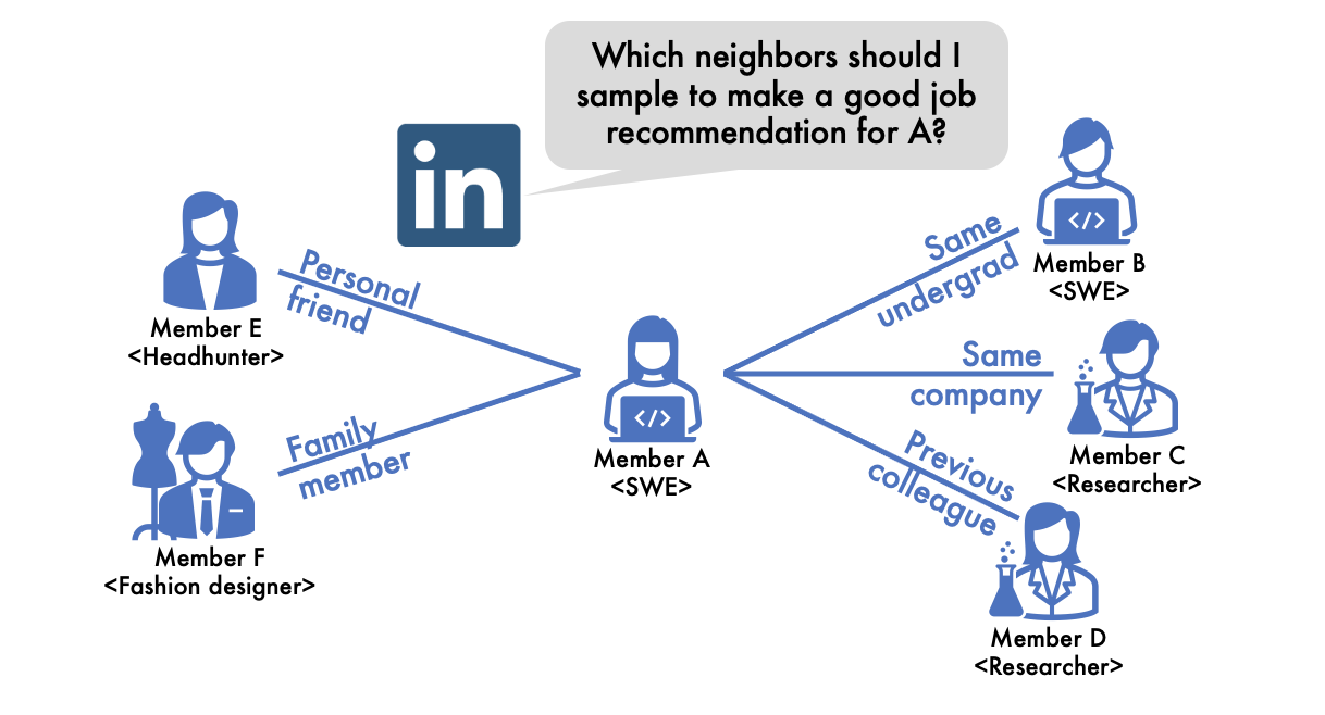
Figure 1: On LinkedIn, people are commonly connected with members from the same field who are likely to share skills and/or job preferences. Graph Convolutional Networks (GCNs) leverage this feature of the LinkedIn network and make better job recommendations by aggregating information from a member’s connections. For instance, to recommend a job to Member A, GCNs will aggregate information from Members B, C, and D who worked/are working in the same companies or have the same major.
TL;DR: Graph Convolutional Networks (GCNs) complement each node embedding with their neighboring node embeddings under a ‘homophily’ assumption, “connected nodes are relevant.” This leads to two critical problems when applying GCNs to real-world graphs: 1) scalability: numbers of neighboring nodes are sometimes too large to aggregate everything (e.g., Cristiano Ronaldo has 358 million connected accounts — his followers — on the Instagram’s member-to-member network), 2) low accuracy: nodes are sometimes connected with irrelevant nodes (e.g., people make connections with their personal friends who work in the totally different fields on LinkedIn). Here, we introduce a performance-adaptive sampling strategy for GCNs to solve both scalability and accuracy problems at once.
Graphs are ubiquitous. Any entities and interactions among them could be presented as graphs — nodes correspond to the individual entities and edges are generated between nodes when the corresponding entities have interactions between them. For instance, there are who-follows-whom graphs in social networks, who-pays-whom transaction networks in banking systems, and who-buys-which-products graphs in online malls. In addition to those originally graph-structured data, recently, few other computer science fields build new types of graphs by abstracting their concept (e.g., scene graphs in computer vision or knowledge graphs in NLP).
What are Graph Convolutional Networks?
As graphs contain rich contextual information — relationships among entities, various approaches have been proposed to include graph information in deep learning models. One of the most successful deep learning models combining graph information is Graph Convolutional Networks (GCNs) [1]. Intuitively, GCNs complement each node embeddings with their neighboring node embeddings, assuming neighboring nodes are relevant (we call this ‘homophily’), thus their information would help to improve a target node’s embedding. In Figure 1, on LinkedIn’s member-to-member networks, we refer to Member A‘s previous/current colleagues to make a job recommendation for Member A, assuming their jobs or skills are related to Member A‘s. GCNs aggregate neighboring node embeddings by borrowing the convolutional filter concept from Convolutional Neural Networks (CNNs) and replacing it with a first-order graph spectral filter.
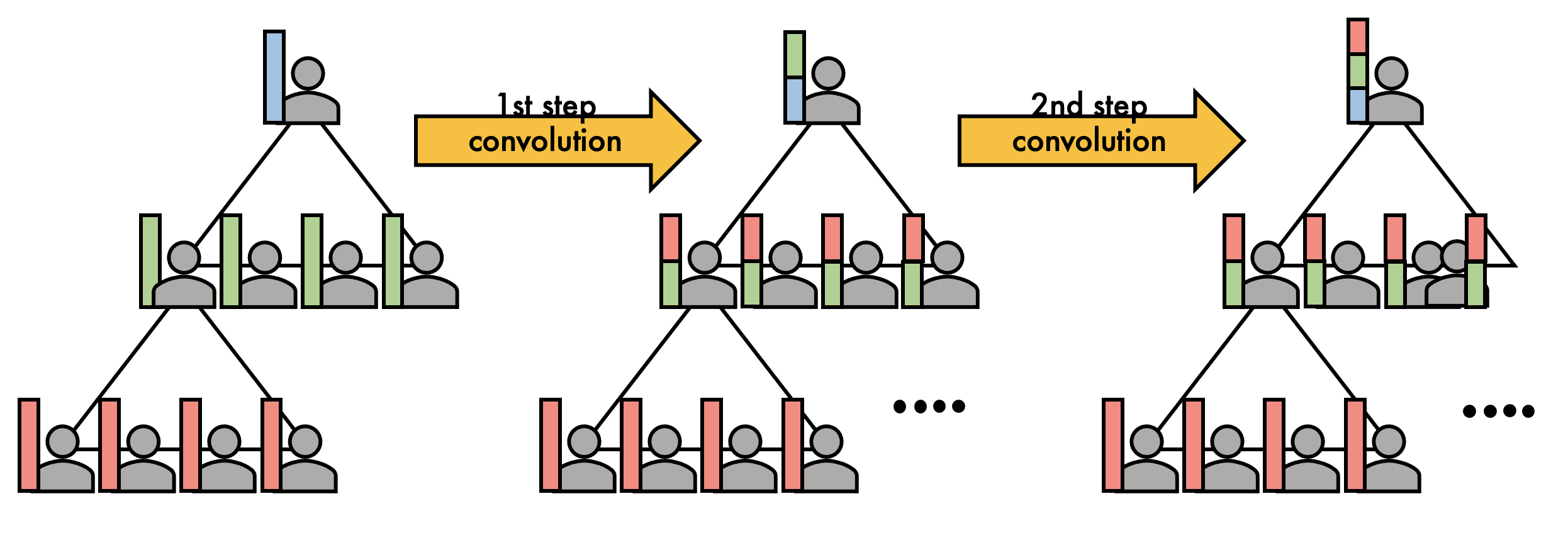
Figure 2. GCNs aggregate neighboring node embeddings to complement each node embeddings in convolution operations. After 2 steps of convolution operations, nodes have information of neighboring nodes within 2 hops.
When (h_i^{(l)}) denotes the hidden embedding of node (v_i) in the (l)-th layer, one-step convolution (we also call it one-step aggregation or one-step message-passing) in GCNs is described as follows:
where (a(v_i, v_j)) =1 when there is an edge from (v_i) to (v_j), otherwise 0; (N(i) = sum_{j=1}^{N} a(v_i, v_j)) is the degree of node (v_i); (alpha(cdot)) is a nonlinear function; (W^{(l)}) is the learnable transformation matrix. In short, GCNs average neighboring nodes (v_j)‘s embeddings (h_j^{(l)}), transform them with (W^{(l)}) and (alpha(cdot)), then update node (v_i)‘s embedding (h_i^{(l+1)}) using the aggregated and transformed neighboring embeddings. In practice, (h_i^{(0)}) is set with input node attributes and (h_i^{(L)}) is passed to an output layer specialized to a given downstream task. By stacking graph convolutional layers (L) times, (L)-layered GCNs complement each node embeddings with its neighboring nodes within (L) hops (Figure 2).
GCNs have garnered considerable attention as a powerful deep learning tool for representation learning of graph data. They demonstrate state-of-the-art performance on node classification, link prediction, and graph property prediction tasks. Currently, GCNs are one of most hot topics in graph mining and deep learning fields.
GCNs do not scale to large-scale real-world graphs.
However, when we adapt GCNs to million or billion-scaled real-world graphs (even trillion-scaled graphs for Google or Facebook), GCNs show a scalability issue. The main challenge comes from neighborhood expansion — GCNs expand neighbors recursively in the aggregation operations (i.e., convolution operations), leading to high computation and memory footprints. For instance, given a graph whose average degree is (d), (L)-layer GCNs access (d^L) neighbors per node on average (Figure 2). If the graph is dense or has many high degree nodes (e.g., Cristiano Ronaldo has 358 million followers on Instagram), GCNs need to aggregate a huge number of neighbors for most of the training/test examples.
The only way to alleviate this neighbor explosion problem is to sample a fixed number of neighbors in the aggregation operation, thereby regulating the computation time and memory usage. We first recast the original Equation (eqref{1}) as follows:
where (p(j|i) = frac{a(v_i, v_j)}{N(i)}) defines the probability of sampling (v_j) given (v_i). Then we approximate the expectation by Monte-Carlo sampling as follows [2]:
where (k) is the number of sampled neighbors for each node. Now, we can regulate the GCNS’ computation costs using the sampling number (k).
GCN performance is affected by how neighbors are sampled, more specifically, how sampling policies — (q(j|i)), a probability of sampling a neighboring node (v_j) given a source node (v_i) — are defined. Various sampling policies [2-5] have been proposed to improve the GCN performance. Most of them target to minimize the variance caused by sampling (i.e., variance of the estimator (h^{(l+1)}_i) in Equation (eqref{3})). Variance minimization makes the aggregation of the sampled neighborhood to approximate the original aggregation of the full neighborhood. In other words, their sampling policies set the full neighborhood as the optimum they should approximate. But, is the full neighborhood the optimum?
Are all neighbors really helpful?
Figure 3. In the real world, we make connections not only with people working in similar fields but also with personal friends or family members who have different career paths in LinkedIn. Which neighbor should we sample to make a better job recommendation?
To answer this question, let’s go back to the motivation of the convolution operation in GCNs. When two nodes are connected with each other in graphs, we regard them as related to each other. Based on this ‘homophily’ assumption, GCNs aggregate neighboring nodes’ embeddings via the convolution operation to complement a target node’s embedding. So the convolution operation in GCNs will shine only when neighbors are informative for the task.
However, real-world graphs always contain unintended noisy neighbors. For example, in LinkedIn’s member-to-member networks, members might make connections not only with her colleagues working in the same field, but also with her family members or personal friends who may have totally different career paths (Figure 3). These family members or personal friends are uninformative for the job recommendation task. When their embeddings are aggregated into the target member’s embedding via the convolution operations, the recommendation quality becomes degraded. Thus, to fully enjoy benefits of the convolution operations, we need to filter out noisy neighbors.
How could we filter out noisy neighbors? We find the answer in the sampling policy: we sample neighbors only informative for a given task. How could we sample informative neighbors for the task? We train a sampler to maximize the target task’s performance (instead of minimizing sampling variance).
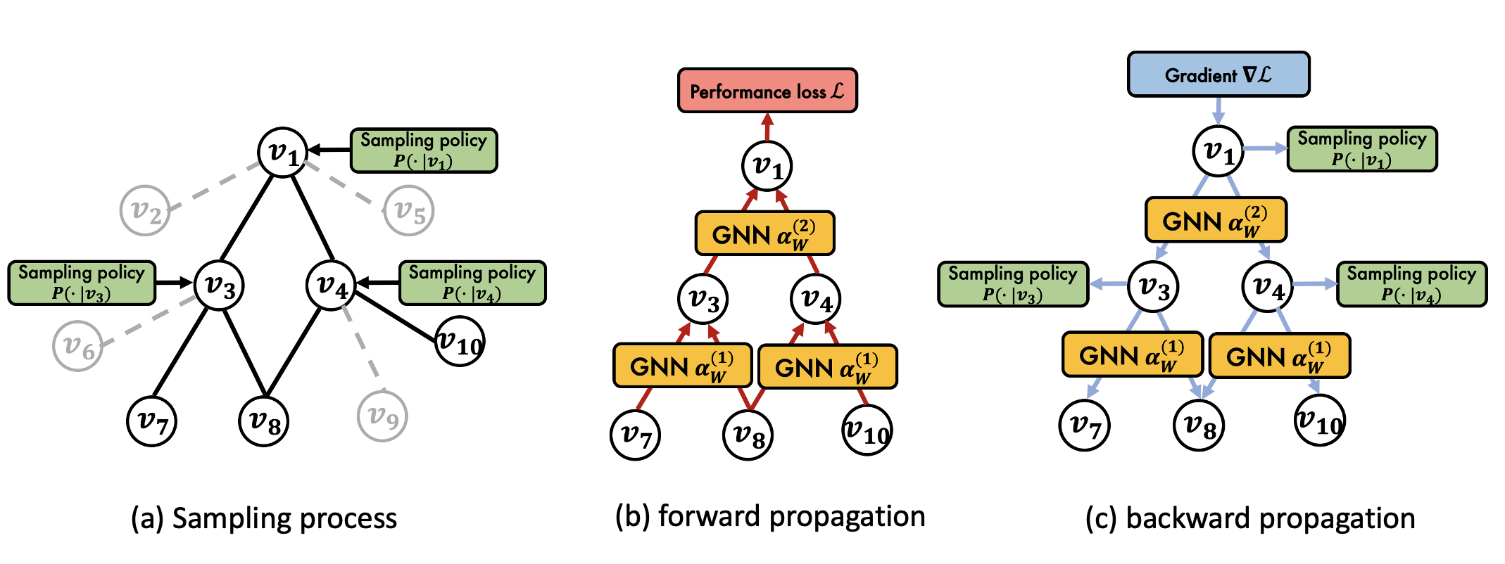
Figure 4. PASS is composed of three steps: (a) sampling, (b) feedforward propagation, and (c) backpropagation. In the backpropagation process, the GCN and the sampling policy are optimized jointly to minimize the GCN performance loss.
PASS: performance-adaptive sampling strategy for GCNs
We propose PASS, a performance-adaptive sampling strategy that optimizes a sampling policy directly for GCN performance. The key idea behind our approach is that we learn a sampling policy by propagating gradients of the GCN performance loss through the non-differentiable sampling operation. We first describe a learnable sampling policy function and how it operates in the GCN. Then we describe how to learn the parameters of the sampling policy by back-propagating gradients through the sampling operation.
Sampling policy: Figure 4 shows an overview of PASS. In the forward pass, PASS samples neighbors with its sampling policy (Figure 4(a)), then propagates their embeddings through the GCN (Figure 4(b)). Here, we introduce our parameterized sampling policy (q^{(l)}(j|i)) that estimates the probability of sampling node (v_j) given node (v_i) at the (l)-th layer. The policy (q^{(l)}(j|i)) is composed of two methodologies, importance (q^{(l)}_{imp}(j|i)) and random sampling (q^{(l)}_{rand}(j|i)) as follows:
where (W_s) is a transformation matrix; (h^{(l)}_i) is the hidden embedding of node (v_i) at the (l)-th layer; (N(i)) is the degree of node (v_i); (a_s) is an attention vector; and (q^{(l)}(cdot|i)) is normalized to sum to 1. (W_s) and (a_s) are learnable parameters of our sampling policy, which will be updated toward performance improvement.
When a graph is well-clustered (i.e., less noisy neighbors), nodes are connected with all informative neighbors. Then random sampling becomes effective since its randomness helps aggregate diverse informative neighbors, thus preventing the GCN from overfitting. By capitalizing on both importance and random samplings, our sampling policy better generalizes across various graphs. Since we don’t know whether a given graph is well-clustered or not in advance, (a_s) learns which sampling methodology is more effective on a given task.
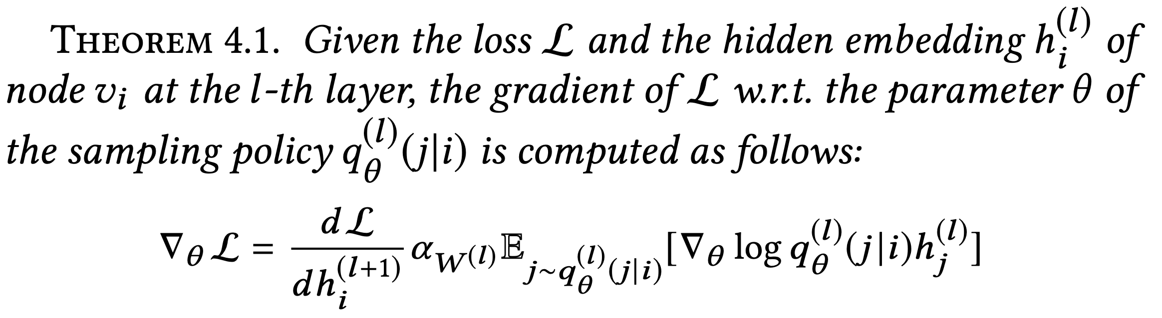
Training the Sampling Policy: after a forward pass with sampling, the GCN computes the performance loss (e.g., cross-entropy for node classification) then back-propagates gradients of the loss (Figure 4(c)). To learn a sampling policy maximizing the GCN performance, PASS trains the sampling policy based on gradients of the performance loss passed through the GCN. When (theta) denotes parameters ((W_s, a_s)) in our sampling policy (q^{(l)}_{theta}), we can write the sampling operation with (q^{(l)}_theta(j|i)) as follows:
[h^{(l+1)}_i = alpha_{W^{(l)}}(mathbb{E}_{jsim q^{(l)}_{theta}(j|i)}[h^{(l)}_j]), quad l = 0,dots,L-1]
Before being fed as input to the GCN transformation (alpha_{W^{(l)}})((cdot)), the hidden embeddings (h^{(l)}_j) go through an expectation operation (mathbb{E}_{jsim q^{(l)}_{theta}(j|i)})[(cdot)] under the sampling policy, which is non-differentiable. To pass gradients of the loss through the expectation, we apply the log derivative trick [6], widely used in reinforcement learning to compute gradients of stochastic policies. Then the gradient (nabla_theta mathcal{L}) of the loss (mathcal{L}) w.r.t. the sampling policy (q^{(l)}_{theta(j|i)}) is computed as follows:
Based on Theorem 4.1, we pass the gradients of the GCN performance loss to the sampling policy through the non-differentiable sampling operation and optimize the sampling policy for the GCN performance. You can find proof of the theorem in our original paper. PASS optimizes the sampling policy jointly with the GCN parameters to minimize the task performance loss, resulting in a considerable performance improvement.
Experimental Results
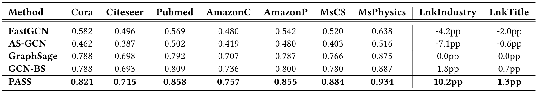
Table 1. PASS outperforms all baselines up to 10.4% on the benchmark datasets and up to 10.2% on LinkedIn production datasets (LnkIndustry, LnkTitle). Results on the benchmark datasets are presented in precision. Results on LinkedIn production datasets are presented in percentage points (pp) with respect to GraphSage (random sampling).
To examine the effectiveness of PASS, we run PASS on seven public benchmarks and two LinkedIn production datasets in comparison to four state-of-the-art sampling algorithms. GraphSage [2] samples neighbors randomly, while FastGCN [3], AS-GCN [4], and GCN-BS [5] do importance sampling with various sampling policy designs. Note that FastGCN, AS-GCN, and GCN-BS all target to minimize variance caused by neighborhood sampling. In Table 1, our proposed PASS method shows the highest accuracy among all baselines across all datasets on the node classification tasks. One interesting result is that GraphSage, which samples neighbors randomly, still shows good performance as compared to carefully designed importance sampling algorithms. The seven public datasets are well-clustered, which means most neighbors are relevant rather than noisy to a target node; thus there is not much room for improvement using importance sampling.
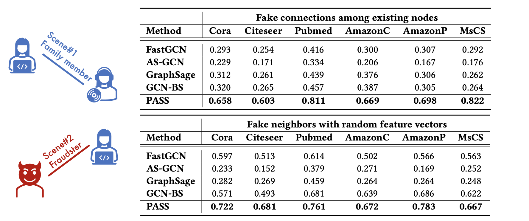
In the following experiment, we add noise to graphs. We investigate two different noise scenarios: 1) fake connections among existing nodes, and 2) fake neighbors with random feature vectors. These two scenarios are common in real-world graphs. The first “fake connection” scenario simulates connections made by mistake or unfit for the purpose (e.g., connections between family members in LinkedIn). The second “fake neighbor” scenario simulates fake accounts with random attributes used for fraudulent activities. For each node, we generate five true neighbors and five fake neighbors.
Table 2. PASS maintains high accuracy in various graph noise scenarios, while the accuracy of all other baselines plummets. PASS is effective not only in sampling informative neighbors but also in removing irrelevant neighbors.
Table 2 shows that PASS consistently maintains high accuracy across all scenarios, while the performance of all other methods plummets. GraphSage, which gives the same sampling probability to true neighbors and fake neighbors, shows a sharp drop in accuracy. Other importance sampling-based methods, FastGCN, AS-GCN, and GCN-BS, also see a sharp drop in accuracy. They target to minimize sampling variance; thus they are likely to sample high-degree or dense-feature nodes, which help stabilize the variance, regardless of their relationship with the target node. Then, they all fail to distinguish fake neighbors from true neighbors. On the other hand, PASS learns which neighbors are informative or fake from gradients of the performance loss. These results show that the optimization of the sampling policy towards performance brings robustness to graph noise.
How does PASS learn which neighbors to sample?
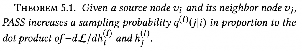
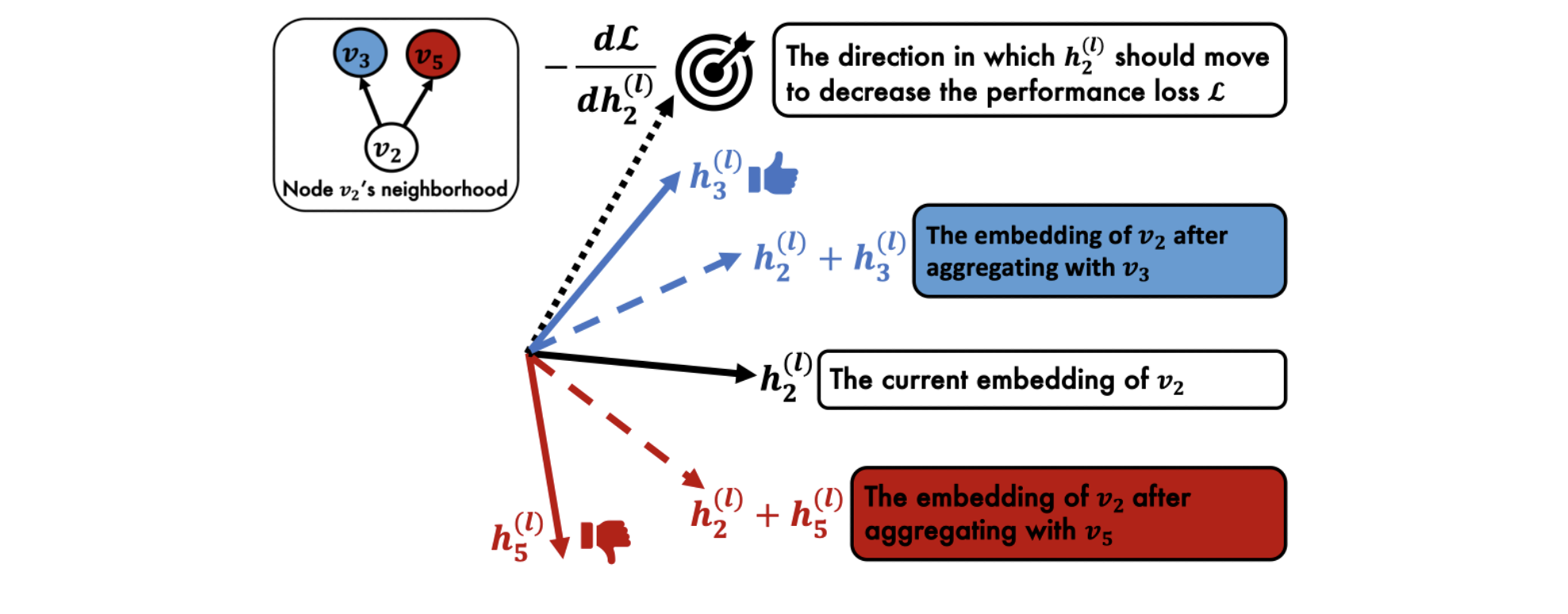
PASS demonstrates superior performance in sampling informative neighbors for a given task. How could PASS learn whether a neighbor is informative for the task? How could PASS decide a certain sampling probability for each neighbor? To understand how PASS actually works, we dissect the back-propagation process of PASS. In Theorem 5.1., we find out that, during the back-propagation phase, PASS measures the alignment between (-dmathcal{L}/dh^{(l)}_i) and (h^{(l)}_j) and increases the sampling probability (q^{(l)}(j|i)) in proportion to this alignment. Proof of Theorem 5.1. can be found in the original paper.
This is an intuitively reasonable learning mechanism. GCNs train their parameters to move the node embeddings (h^{(l)}_i) in the direction that minimizes the performance loss (mathcal{L}), i.e., the gradient (-dmathcal{L} / dh^{(l)}_i). PASS promotes this process by sampling neighbors whose embeddings are aligned with the gradient (-dmathcal{L}/dh^{(l)}_i). When (h^{(l)}_i) is aggregated with the embedding (h^{(l)}_j) of a sampled neighbor aligned with the gradient, it moves in the direction that reduces the loss (mathcal{L}).
Figure 5. Interpretation of why PASS assigns higher sampling probability to node (v_3) than (v_5) given target node (v_2). Node (v_3)’s embedding (h^{(l)}_3) helps (v_2)’s embedding (h^{(l)}_2) move in the direction (-dmathcal{L} / dh^{(l)}_2) that decreases the performance loss (mathcal{L}), while aggregating with node (v_5)’s embedding would move (h^{(l)}_2) in the opposite direction.
Let’s think about a simple example. In Figure 5, (h^{(l)}_3) is better aligned with (-dmathcal{L}/dh^{(l)}_2) than (h^{(l)}_5). Then PASS considers (v_3) more informative than (v_5) for (v_2) because node (v_3)’s embedding (h^{(l)}_3) helps (v_2)’s embedding (h^{(l)}_2) move in the direction (-dmathcal{L} / dh^{(l)}_2) that decreases the performance loss (mathcal{L}), while aggregating with node (v_5)’s embedding would move (h^{(l)}_2) in the opposite direction.
This reasoning process leads to two important considerations. First, it crystallizes our understanding of the aggregation operation in GCNs. The aggregation operation enables a node’s embedding to move towards its informative neighbors’ embeddings to reduce the performance loss. Second, this reasoning process shows the benefits of joint optimization of the GCN and sampling policy. Without optimizing the sampling policy jointly, the GCN depends solely on its parameters to move node embeddings towards the minimum performance loss. Joint optimization with the sampling policy helps the GCN to move the node embeddings more efficiently by aggregating with informative neighbors’ embeddings, leading to the minimum loss more efficiently.
PASS catches two birds, “accuracy” and “scalability”, with one stone.
Figure 6. PASS achieves both accuracy and scalability using a performance-adaptive sampling strategy.
Today, we introduced a novel sampling algorithm PASS for graph convolutional networks. By sampling neighbors informative for task performance, PASS improves both the accuracy and scalability of CGNs. In nine different real-world graphs, PASS consistently outperforms state-of-the-art samplers, being up to 10.4% more accurate. In the presence of graph noises, PASS shows up to 53.1% higher accuracy than the baselines, proving its ability to read the context and distinguish the noises. By dissecting the back-propagation process, PASS explains why a neighbor is considered informative and assigned a high sampling probability.
In this era of big data, new graphs and tasks are generated every day. Graphs become bigger and bigger, and different tasks require different relational information within the graphs. By sampling informative neighbors adaptively for a given task, PASS allows GCNs to be applied on larger-scale graphs and a more diverse range of tasks. We believe that PASS can bring even more impact on a wider range of users across academia and industry in the future.
Links: paper, video, slide, code will be released at the end of 2021.
If you would like to reference this article in an academic publication, please use this BibTeX:
@inproceedings{yoon2021performance,
  title={Performance-Adaptive Sampling Strategy Towards Fast and Accurate Graph Neural Networks},
  author={Yoon, Minji and Gervet, Th{'e}ophile and Shi, Baoxu and Niu, Sufeng and He, Qi and Yang, Jaewon},
  booktitle={Proceedings of the 27th ACM SIGKDD Conference on Knowledge Discovery & Data Mining},
  pages={2046--2056},
  year={2021}
}
References
Thomas N Kipf and Max Welling. 2016. Semi-supervised classification with graph convolutional networks. arXiv preprint arXiv:1609.02907 (2016).
Will Hamilton, Zhitao Ying, and Jure Leskovec. 2017. Inductive representation learning on large graphs. In Advances in neural information processing systems.
Jie Chen, Tengfei Ma, and Cao Xiao. 2018. Fastgcn: fast learning with graph convolutional networks via importance sampling. arXiv preprint arXiv:1801.10247 (2018).
Wenbing Huang, Tong Zhang, Yu Rong, and Junzhou Huang. 2018. Adaptive sampling towards fast graph representation learning. In Advances in neural information processing systems. 4558–4567
Ziqi Liu, Zhengwei Wu, Zhiqiang Zhang, Jun Zhou, Shuang Yang, Le Song, and Yuan Qi. 2020. Bandit Samplers for Training Graph Neural Networks. arXiv preprint arXiv:2006.05806 (2020).
Ronald J Williams. 1992. Simple statistical gradient-following algorithms for connectionist reinforcement learning. Machine learning 8, 3-4 (1992), 229–256.
Fig. 1: The safety envelope (in green) is an imaginary surface that separates the robot from all obstacles in its environment. As long as the robot never intersects the safety envelope, it is guaranteed to not collide with any obstacle. Our task is to estimate this envelope.
Safe navigation and obstacle detection
Consider the scene in Fig. 1 that a mobile robot wishes to navigate safely. The scene contains many obstacles such as walls, poles, and walking people. Obstacles could be arbitrarily distributed, their motion might be haphazard, and they may enter and leave the environment in an undetermined manner. This situation is commonly encountered in a variety of robotics tasks such as indoor and outdoor robot navigation, autonomous driving, and robot delivery. The robot must accurately and reliably detect all obstacles (static and dynamic) in the scene to avoid colliding with them and navigate safely. Therefore, it must estimate the safety envelope of the scene.
What is a safety envelope?
We define the safety envelope as an imaginary surface that separates the robot from all obstacles in its environment. As long as the robot never intersects the safety envelope, it is guaranteed to not collide with any obstacles! How can the robot accurately estimate the location of the safety envelope? Can it provide any guarantees about its ability to discover obstacles? In our recent paper published at RSS 2021, we answer these questions in the affirmative using a novel sensor called programmable light curtains.
What are light curtains?
Fig. 2: Comparing a standard LiDAR sensor and a programmable light curtain. A LiDAR detects points in the entire scene but sparsely. A light curtain detects points that intersect a user-specified surface at a much higher resolution.
A programmable light curtain is a 3D sensor recently invented at CMU. It can measure the depth of any user-specified 2D vertical surface (“curtain”) in the environment. A common strategy for 3D sensing is to use LiDARs. LiDARs have become ubiquitous in robotics and autonomous driving. However, they can be low resolution, expensive and slow. In contrast, light curtains are relatively inexpensive, faster, and of much higher resolution!
Most importantly, light curtains are a controllable sensor: the user selects a vertical 2D surface, and the light curtain detects objects intersecting that surface. This is a fundamentally different sensing paradigm from LiDARs. LiDARs passively sense the entire scene without any user input. However, light curtains can be actively controlled by the user to focus their sensing capacity on specific regions of interest. While controllability is clearly a desirable feature, it also presents a unique challenge: light curtains require the user to select which locations to sense. How should we place light curtains to accurately estimate the safety envelope of a scene?
Random curtains can reliably discover obstacles
Fig. 3: A heist scene from the movie Ocean’s Twelve. The robber needs to try extremely hard to avoid intersecting the randomly moving lasers. The same principle applies to randomly placed light curtains: they detect (sufficiently large) obstacles with very high probability. It is virtually impossible to evade random curtains!
Suppose we have a scene with no prior knowledge of where the obstacles are. How should we place light curtains to discover them? Surprisingly, we answered this question by taking inspiration from heist films such as Ocean’s Twelve. In a scene from this movie shown in Fig. 3, the robber attempts to evade a museum’s security system consisting of randomly moving laser detectors. The robber needs to try extremely hard, literally bending over backward, to avoid intersecting the lasers. Although the robber managed to pull it off in the movie, it is clear that this would be virtually impossible in the real world.
Fig. 4: Examples of random light curtains (in blue). The points on the obstacles that are intersected and detected by random curtains are shown in green. Random curtains are able to detect obstacles with high probability.
Light curtains are nothing but moving laser detectors! Therefore, our insight is to place curtains at randomlocations in the scene. We refer to them as “random curtains”, as shown in Fig. 4. It turns out to be incredibly hard for (sufficiently large) obstacles to avoid getting detected by random curtains. We place random curtains to quickly discover unknown objects and estimate the safety envelope of the scene.
In the section on theoretical analysis of random curtains near the end of this blog post, we will present a novel analytical technique that actually computes the probability of random curtains intersecting and detecting obstacles. The analytical probabilities act as safety guarantees for our perception system towards detecting and avoiding obstacles.
Forecasting safety envelopes
Fig. 5 We wish to estimate the safety envelope of a dynamic scene across time. Once the envelope is estimated in the current timestep, we use a machine learning-based forecasting model to predict the change in the location of the safety envelope. This allows us to efficiently track the safety envelope.
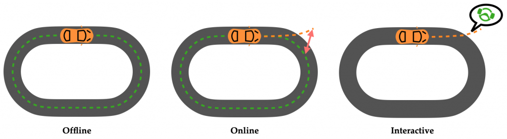
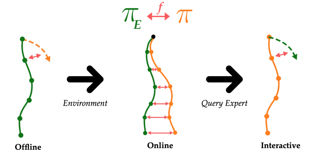
Assume that we have already estimated the safety envelope in the current timestep. As objects move and the scene changes with time, we wish to estimate the safety envelope for the next timestep. In this case, it may be inefficient to explore the scene from scratch by randomly placing curtains. Instead, we use machine learning to train a neural network to forecast how the safety envelope will evolve in the next timestep. The inputs to the network are all light curtain measurements from previous timesteps. The output is the predicted change in the envelope’s position in the next timestep. We use DAgger [Ross et. al. 2011], a standard imitation learning algorithm, to train such a forecasting model from data. By predicting how the safety envelope will move, we can directly sense the locations where obstacles are anticipated to be and efficiently track the safety envelope.
Active light curtain placement pipeline
Fig. 6: Our pipeline for estimating the safety envelope of a dynamic scene. It combines two components: a machine learning-based forecasting model to predict how the envelope will move, and random curtain placements to discover obstacles and update the predictions. Light curtains are also placed to sense the predicted location of the envelope.
Our overall pipeline for placing light curtains to estimate and track the safety envelope is as follows. Given previous light curtain measurements, we train a neural network to forecast how the safety envelope of the scene will evolve in the next timestep. We then place light curtains to sense the predicted locations. At the same time, we place random light curtains to discover obstacles and update our predictions. Finally, the light curtain measurements are input back to the forecasting method, closing the loop.
Real-world results
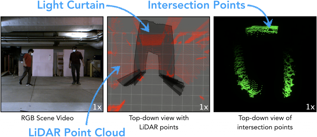
Here is our method in action in the real world! The scene consists of multiple people walking in front of the light curtain device at various speeds and in different patterns. Our method, which combines learning-based forecasting and random curtain placement, tries to estimate the safety envelope of this dynamic scene at each timestep.
The middle video shows the light curtain placed at the estimated location of the safety envelope in black. It also shows a LiDAR point cloud in red, used only for visualization purposes (our method only uses light curtain measurements). The video on the right shows intersection points, i.e. the points detected by the light curtain when it intersects object surfaces in green. These are aggregated across multiple frames to visualize the motion of obstacles.
Brisk Walking
Relaxed Walking
Many people (structured walking)
Many people (haphazard, occluded walking)
Fast motion
In all of the above videos, the light curtain is able to accurately estimate the safety envelope and produce a large number of intersection points. Due to the guarantees of high detection probability, our method generalizes to a varying number of obstacles (one vs. two vs. five people), a large range of motion (relaxed vs. brisk vs. extremely fast and sudden motion), and different patterns of motion (structured vs. complicated and haphazard).
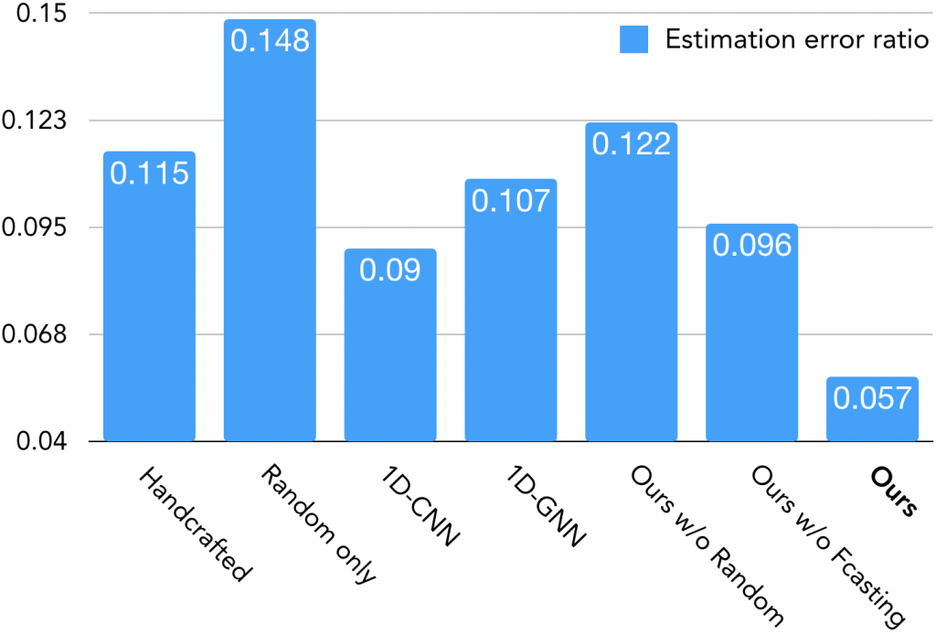
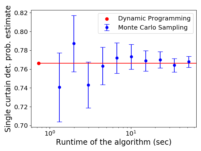
Fig. 7: Quantitative analysis of safety envelope estimation, compared to various baselines.
Fig. 7 shows a quantitative analysis of our method compared to various baselines. We compute the Huber loss (related to the “smooth-L1 loss“) of the ratio between the predicted and true safety envelope location. We compare against a non-learning based handcrafted baseline. The baseline carefully alternates between moving the light curtain forward and backward, resulting in “hugging” the obstacles. We also compare against using only random curtains and using various neural network architectures. We include ablation experiments that remove one component of our method at a time (random curtains and forecasting) to demonstrate that both are crucial to our performance. Our method outperforms all baselines. Please see our paper for more experiments and evaluation metrics.
Theoretical analysis of random curtain detection
Previously, we mentioned that random light curtains can detect obstacles with a high probability. Can we perform any theoretical analysis to actually compute this probability? Can we compute the probability of a random curtain detecting an obstacle of a given shape, size, and location? If so, these probabilities can act as safety guarantees that help certify the ability of our perception system to detect and avoid obstacles. Before we begin analyzing random curtains, we must first understand how they are generated.
Constraint Graph and generating random curtains
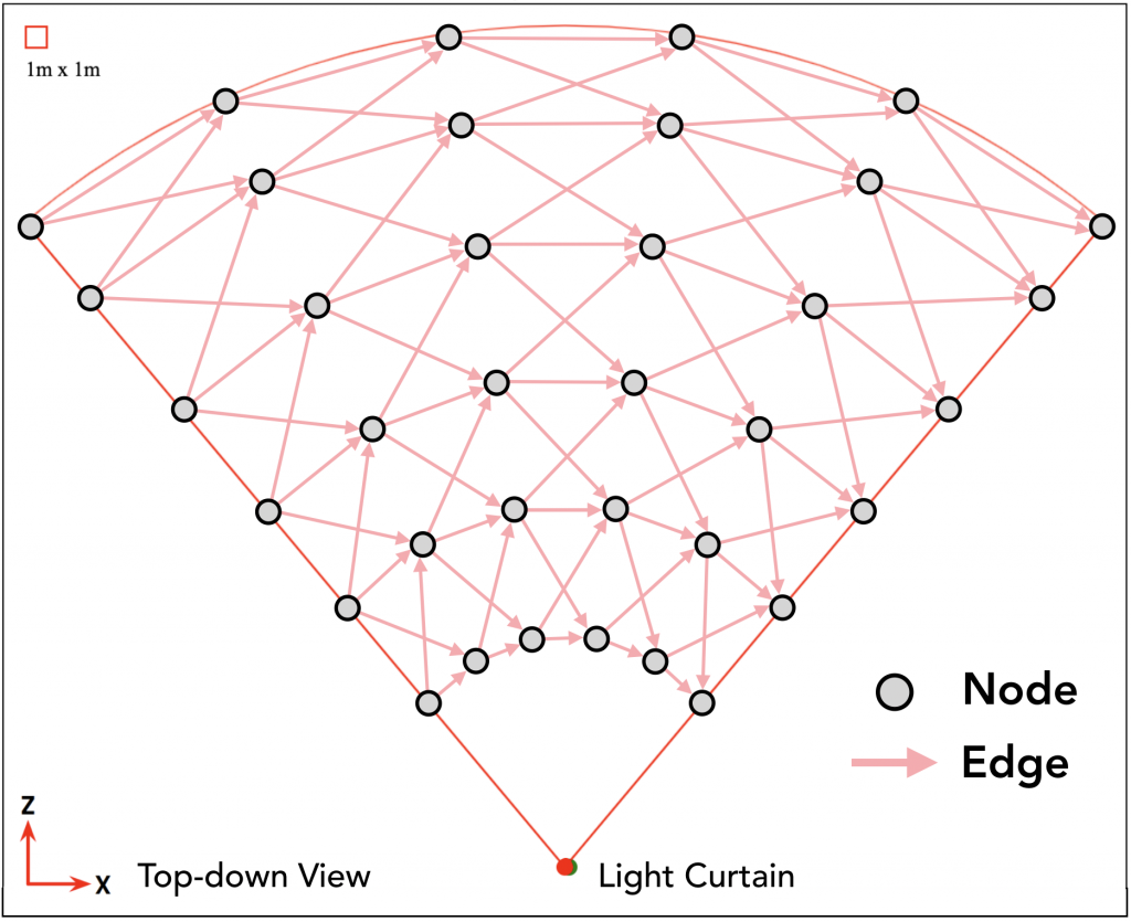
Fig. 8: The constraint graph from the top-down view. Nodes correspond to locations that can be imaged. Two nodes are connected by an edge if they can be imaged sequentially while satisfying the physical constraints of the light curtain device.
In order to generate any light curtain, we need to account for the physical constraints of the light curtain device. These are encoded into a constraint graph (see Fig. 8). The nodes of the graph represent locations where the light curtain might be placed. The nodes are organized into “camera rays” indexed by (t in {1, dots, T}) from left to right. A light curtain is created by imaging one node per ray, from left to right. An edge exists between two nodes if they can be imaged consecutively.
Fig. 9: Any path in the constraint graph represents a feasible light curtain. Random curtains can be generated by performing random walks in the graph.
What decides whether an edge exists between two nodes? The light curtain device contains a rotating mirror that redirects and shoots light into the scene. By specifying the angle of rotation, light can be beamed at the desired locations to be imaged. However, the mirror, being a physical device, has velocity and acceleration limits. Therefore, we add an edge between two nodes only if the mirror can rotate fast enough to image those two locations one after the other.
This means that any path in the constraint graph connecting the leftmost ray (t=1) to the rightmost ray (t=T) represents a feasible light curtain! Furthermore, random curtains can be generated by performing a random walk through the graph. The random walk is performed by starting from a node on the leftmost ray. In each iteration, a node on the next ray is randomly sampled among the neighbors of the current node from some probability distribution (e.g. uniform distribution). This process is repeated till the rightmost ray is reached. Fig. 9 shows examples of actual random curtains generated this way.
Computing detection probability using Dynamic Programming
Fig. 10 Given an obstacle (in blue and red), some random curtains detect the obstacle (in yellow) but some don’t. We wish to compute the probability of detection.
Assume that we are given the shape, size, and location of an obstacle (blue–red shape in Fig. 10). Some random curtains will intersect and detect the obstacle (detections are shown in yellow), but other random curtains will miss the obstacle. Can we compute the probability of detection?
A naive approach would be to enumerate the set of all feasible light curtains and sum the probabilities of sampling those curtains that detect the object. Unfortunately, this is impractical because the number of feasible curtains is exponentially large! Another approach is to use Monte Carlo sampling for estimating the detection probability. In this method, we sample a large number of random curtains and output the fraction of the sampled curtains that detect the obstacle. While this approach is simple, we will show later that it requires a large number of samples to be drawn, and only produces stochastic estimates of the true probability.
Instead, we have developed an analytical and efficient approach to compute the detection probability, using dynamic programming. We first divide the overall problem into multiple sub-problems. Let us represent (mathbf{x}_t) to be a node on the (t)-th ray. Let us define (P_mathrm{det}(mathbf{x}_t)) to be the the probability that “sub-curtains” i.e. partial random curtains starting from node (mathbf{x}_t) and ending at a rightmost node will detect the obstacle. We wish to compute (P_mathrm{det}(cdot)) for every node in the constraint graph. Conveniently, these sub-problems satisfy a recursive relationship! If the obstacle is detected at node (mathbf{x}_t), (P_mathrm{det}(mathbf{x}_t)) is trivially equal to (1). If not, it is equal to the sum of detection probabilities of sub-curtains starting at (mathbf{x}_t)’s child nodes (mathbf{x}_{t+1}), weighted by the probability (P(mathbf{x}_t rightarrow mathbf{x}_{t+1})) of transitioning to (mathbf{x}_{t+1}). This is expressed by the equation below.
Fig. 11: Dynamic programming exploits the structure of the constraint graph to efficiently and analytically compute the overall detection probability. It recursively iterates over all nodes and edges in the graph only once, from right to left.
In order to apply dynamic programming, we start at nodes on the rightmost ray (T). (P_mathrm{det}(cdot)) for these nodes is simply (1) or (0), depending on whether the obstacle is detected at these locations or not. Then, we iterate over all nodes in the graph from right to left (see Fig. 11) and apply the recursive formula in Eqn. 1. Once we have the sub-curtain detection probabilities for the leftmost nodes, the overall detection probability is simply (sum_{mathbf{x}_1} P_mathrm{init}(mathbf{x}_1)~P_mathrm{det}(mathbf{x}_1)), where (P_mathrm{init}(mathbf{x}_1)) is the probability of sampling (mathbf{x}_1) as the starting node of the random curtain.
Note that our method computes the true detection probability precisely — there is no stochasticity or noise in the estimates. It is also very efficient: we only need to iterate over all nodes and edges in the graph once.
An example of random curtain analysis
Fig. 12: The probability of detecting an average-sized car and an average-sized pedestrian by random curtains, as a function of the time taken to place multiple random curtains. The detection probability increases exponentially as more random curtains are placed.
Let us look at an example of random curtain analysis in Fig. 12. The X-axis shows the time taken to place multiple random curtains at 60 Hz. The Y-axis shows the detection probability of an average-sized car and an average-sized pedestrian. Average sizes were computed from KITTI, a large-scale autonomous driving benchmark dataset. Let (p) be the probability of detecting an obstacle by a single random curtain. If (n) curtains are sampled independently and placed, the probability that at least one of them will detect the object is (1-(1-p)^n), which increases exponentially with (n). Thanks to the high speed of light curtains, within as low as 67 milliseconds, we are able to guarantee the detection of an average-sized pedestrian with more than 95% probability and an average-sized car with more than 99% probability!
Comparison to sampling-based estimation
Fig. 13: Comparing the speed and precision of estimating the random curtain detection probability using dynamic programming (our method) and Monte Carlo sampling.
In traditional Monte Carlo estimation, we sample a large number of random curtains by performing multiple forward passes through the constraint graph. Then, we output the fraction of the sampled curtains that detect the obstacle. This produces an unbiased estimate of the detection probability, with a variance that decreases with the number of samples used. Fig. 13 show the estimates produced by each method with 95% confidence intervals, versus their runtime (in log-scale). Monte Carlo (MC) sampling produces noisy estimate of the true probability whereas our dynamic programming (DP) approach produces precise estimates (zero uncertainty); such precise estimates are useful for reliably evaluating the safety and robustness of our perception system. Furthermore, DP is orders of magnitude faster (takes 0.8 seconds) than MC since MC requires a large number of samples to converge to our estimate.
We have created an interactive web-based demo of random curtain analysis! The user can draw any shape, size, and location of the obstacle. The demo runs dynamic programming to compute the random curtain detection probability and displays the analysis. The demo also generates random curtains and visualizes detections of the obstacle. Click on the link to check it out!
Conclusion
We presented a method to estimate the safety envelope of a scene: a hypothetical surface that separates the robot from all obstacles in the environment. We used programmable light curtains, an actively controllable, resource-efficient sensor to directly estimate the safety envelope. Using a dynamic programming-based approach, we showed that random light curtains can discover obstacles with high-probability guarantees. We combined this with a machine learning-based forecasting method to efficiently track the safety envelope. This enables our robot perception system to accurately estimate safety envelopes, while our probabilistic guarantees help certify its accuracy and safety. This work is a step towards safe robot navigation using inexpensive controllable sensors.
Further reading
If you’re interested in more details, please check out the links to the full paper, the project website, talk, demo, and more!
This material is based upon work supported by the National Science Foundation under Grants No. IIS-1849154, IIS-1900821 and by the United States Air Force and DARPA under Contract No. FA8750-18-C-0092. All opinions, findings, and conclusions or recommendations expressed in this post are those of the author(s) and do not necessarily reflect the views of Carnegie Mellon University, National Science Foundation, United States Air Force and DARPA.
Imitation learning (IL) is the problem of finding a policy, (pi), that is as close as possible to an expert’s policy, (pi_E). IL algorithms can be grouped broadly into (a) online, (b) offline, and (c) interactive methods. We provide, for each setting, performance bounds for learned policies that apply for all algorithms, provably efficient algorithmic templates for achieving said bounds, and practical realizations that out-perform recent work.
From beating the world champion at Go (Silver et al.) to getting cars to drive themselves (Bojarski et al.), we’ve seen unprecedented successes in learning to make sequential decisions over the last few years. When viewed from an algorithmic viewpoint, many of these accomplishments share a common paradigm: imitation learning (IL). In imitation learning, one is given access to samples of expert behavior (e.g. moves chosen by Monte-Carlo Tree Search or steering angles recorded from an expert driver) and tries to learn a policy that mimics this behavior. Unlike reinforcement learning, imitation learning does not require careful tuning of a reward function, making it easier to scale to real-world tasks where one is able to gather expert behavior (like Go or driving). As we continue to apply imitation learning algorithms to safety-critical problems, it becomes increasingly important for us to have strong guarantees on their performance: while wrong steps in Go lead to a lost game at worst, mistakes of self-driving cars could result in far worse. In our ICML’21 Paper Of Moments and Matching: A Game Theoretic Framework for Closing the Imitation Gap, we provide bounds on how well any imitation algorithm can do, as well as provably efficient algorithms for achieving these bounds.
A Taxonomy of Imitation Learning Algorithms
Let’s focus on the problem of trying to teach a car to drive around a track from expert demonstrations. We instrument the car with cameras and sensors that measure the angle of the wheel and how hard the pedals are being pushed. Then, in terms of increasing requirements, the approaches we could take are:
Offline: Have the expert drive laps, recording their states (camera images) and actions (pedals/wheel). Use your favorite supervised learning algorithm to regress from states to actions. This approach is called Behavioral Cloning.
Online: Record expert states and actions. Then, have the car try to drive around the track and measure the delta between learner and expert trajectories. Train the policy to minimize this delta. GAIL is an algorithm that uses a discriminator network to measure this delta.
Interactive: (0) Start with an empty dataset D. (1) Record the car driving a sample lap. (2) Ask the expert driver what they would have done for each recorded image. Append this data to D. (3) Regress over data in D. (4) Go back to 1. This approach is known as DAgger.
One of our key insights is that all three of these approaches can be seen as minimizing a sort of divergence from expert behavior. Concretely,
Offline: We measure a divergence between learner and expert actions on states from expert demonstrations.
Online: We measure a divergence between learner and expert trajectories.
Interactive: We measure a divergence between learner and expert actions but on states from learner rollouts.
Also notice that as we transition from Offline to Online IL, we add a requirement of access to the environment or an accurate simulator. As we move from Online to Interactive IL, we also need access to a queryable expert. Let (pi) denote the policy, (pi_E) denote the expert’s policy, and (f) denote the divergence. We can visualize our thoughts thus far as:
With this divergence-minimizing perspective in mind, we’re able to introduce a unifying, game-theoretic perspective.
A Game-Theoretic Perspective on IL
A natural question at this point might be: what divergence should one use to measure the difference between learner and expert behavior? Examples abound in the literature: Kullback-Liebler? Wasserstein? Jensen-Shannon? Total Variation? Maximum Mean Discrepancy? Without prior knowledge about the problem, it’s really hard to say. For example, KL Divergence has a mode-covering effect — this means that if half the data was the expert swerving left to avoid a tree and half the data was them swerving right, the learner would learn to pick a point in the middle and drive straight into the tree!
If we’re not sure what divergence is the right choice, we can just minimize all of them, which is equivalent to minimizing a worst-case or adversarially-chosen one. Using (pi) and (pi_E) to denote the learner and expert policies, we can write out the optimization problem for each setting:
Online: $$ min_{pi} max_f mathbb{E}_{s, a sim pi}[f(s, a)] – mathbb{E}_{s, a sim pi_E}[f(s, a)]$$
Interactive: $$ min_{pi} max_f mathbb{E}_{s, a sim pi}[f(s, a) – f(s, pi_E(s))] $$
Each of these equations is in the form of a two-player zero-sum game between a learner (pi) and a discriminator (f). Two-player zero-sum games have been extensively studied in game theory, allowing us to use standard tools to analyze and solve them. Notice the similarity of the forms of these games — the only real difference is which state-action distributions the divergence is calculated between. Thus, we can view all three classes of imitation learning as solving a games with different classes of discriminators. This game-theoretic perspective is extremely powerful for a few reasons:
As we have access to more information (e.g. a simulator or a queryable expert), we’re able to evaluate more powerful discriminators. Minimizing these more powerful discriminators leads to tighter performance bounds. Specifically, we show that the difference between learner and expert performance for offline IL scales quadratically with the horizon of the problem, and linearly for online / interactive IL. Quadratically compounding errors translate to poor real-world performance. Thus, one perspective on our bounds is that they show that access to a simulator or a queryable expert is both necessary and sufficient for learning performant policies. We recommend checking out the full paper for the precise upper and lower bounds.
These performance bounds apply for all algorithms in each class — after all, you can’t do better by considering a more restrictive class of divergences. This means our bounds apply for a lot of prior work (e.g. Behavioral Cloning, GAIL, DAgger, MaxEnt IRL, …). Importantly, these bounds also apply for all non-adversarial algorithms: they’re just optimizing over a singleton discriminator class.
Our game-theoretic perspective also tells us that finding a policy that minimizes the worst-case divergence is equivalent to finding a Nash Equilibrium of the corresponding game, a problem we know how to solve provably efficiently for two-player zero-sum games. By solving a particular game, we inherit the performance bounds that come with the class of divergences considered.
Together, these three points tell us that a game-theoretic perspective allows us to unify imitation learning as well as efficiently find strong policies!
A Practical Prescription for each IL Setting
Let’s dig into how we can compute Nash equilibria efficiently in theory and in practice for all three games. Intuitively, a Nash equilibrium is a strategy for each player such that no player wants to unilaterally deviate. This means that each player is playing a best-response to every other player. We can find such an equilibrium by competing two types of algorithms:
No-Regret: slow, stable, choosing best option over history.
Best-Response: fast, choosing best option to last iterate of other player.
Classic analysis shows that having one player follow a no-regret algorithm and the other player follow a best-response algorithm will, within a polynomial number of iterations, converge to an approximate Nash equilibrium of the game. The intuition of the proof is that if player 1 is steadily converging to a strategy that performs well even when player 2 choses their strategy adversarially, player 1 can’t have much of an incentive to deviate, meaning their strategy must be half of a Nash equilibrium.
We’d like to emphasize the generality of this approach to imitation learning: you can plug in any no-regret algorithm and both our policy performance and efficiency results still hold. There’s a plethora of algorithms that can be developed from this no-regret reduction perspective!
We instantiate this general template into an implementable procedure for each setting. We compare our approaches against similar recent work. We plot the performance of our methods in orange. (J(pi)) refers to learner’s expected cumulative reward while (pi_E) in green is the expert’s performance. As stated above, our goal is for the learner to match expert performance.
Offline: We adopt a model similar to a Wasserstein GAN where the learner acts as the generator and the discriminator tries to distinguish between learner and expert actions on expert states. We set the learner’s learning rate to be much lower than that of the discriminator, simulating no-regret on policy vs. best response on divergence. We term this approach Adversarial Value-moment IL, or AdVIL. We find it to be competitive with recent work:
Online: We repurpose the replay buffer of an off-policy RL algorithm as the discriminator by assigning negative rewards to actions that don’t directly match the expert. We impute a reward of +1 for expert behavior and -1/k for learner behavior from a past round, where k is the round number. The slow-moving append-only replay buffer implements a no-regret algorithm against a policy that best-responds via RL at each round. We term this approach Adversarial Reward-moment IL, or AdRIL, and find that it can significantly outperform other online IL algorithms at some tasks:
Interactive: We modify DAgger to use adversarially chosen losses at each round instead of a fixed function. At each round, a discriminator network is trained between the last policy and the expert. Then, for all samples for that round, this discriminator network is used as the loss function. Then, just like DAgger, the learner minimizes loss over the history of samples and loss functions for all rounds. Thus, the learner is following a no-regret algorithm against a best-response by the discriminator. We call this algorithm DAgger-esque Qu-moment IL, or DAeQuIL.
To demonstrate the potential advantages of DAeQuIL over DAgger, we test out both algorithms on a simulated UAV forest navigation task, where the expert demonstrates a wide variety of tree avoidance behaviors (left). DAgger attempts to match the mean of these interactively queried action labels, leading to it learning to crash directly into the first tree it sees (center). DAeQuIL, on the other hand, is able to learn to swerve out of the way of trees and navigate successfully through the forest (right).
Parting Thoughts
We provide, for all three settings of imitation learning, performance bounds for learned policies, a provably efficient reduction to no-regret online learning, and practical algorithms. If you’re interested in learning more, I recommend you check out:
There are lots of interesting areas left to explore in imitation learning, including imitation from observation alone that would allow one to leverage the large corpus of instructional videos online to train robots. Another direction that we’re particularly excited about is mimicking expert behavior, even in the presence of unobserved confounders. Stay tuned!
DISCLAIMER: All opinions expressed in this post are those of the author and do not represent the views of CMU.
Figure 1: Overview: To avoid out-of-distribution actions in the Offline Reinforcement Learning problem, we propose to implicitly constrain the policy by modifying the action space instead of enforcing explicit constraints. The policy is trained to output a latent action which will be passed into a decoder pretrained with the dataset. We demonstrate that our method provides competitive performance in both simulation and real-robot experiments.
Offline RL: Learning a policy from a static dataset
The goal of Reinforcement Learning (RL) is to learn to perform a task by interacting with the environment. It has achieved significant success in a lot of applications such as games and robotics. One major challenge in RL is that it requires a huge amount of interactive data collected in the environment to learn a policy. However, data collection is expensive and potentially dangerous in many real-world applications, such as robotics in safety-critical situations (e.g., around humans) or healthcare problems. Worse, RL algorithms also usually assume that the dataset used to update the policy comes from the current policy or its own training process.
To use data more wisely, we may consider Offline Reinforcement Learning. The goal of offline RL is to learn a policy from a static dataset of transitions without further data collection. Although we may still need a large amount of data, the assumption of static datasets allows more flexibility in data collection. For example, in robotics, we can include human demonstrations, reuse rollouts from previous experiments, and share data within the community. In this way, the dataset is more likely to be scaled up in size even when data collection is expensive.
Figure 2: In contrast to a common reinforcement learning pipeline that collects data and updates the policy alternatively, Offline Reinforcement Learning aims to learn a policy from a static dataset without further data collection.
One important feature of offline RL is that it requires no assumption about the performance of the policy that is used to collect the dataset. This is in contrast to behavior cloning, where we assume that the dataset is collected by an expert, so that we can directly “copy” the actions given states without reasoning about the future reward. In offline RL, the dataset could be collected by a policy (or several policies) with arbitrary performance.
At first glance, off-policy algorithms seem to be able to meet the above requirements. Off-policy algorithms save the agent’s interactions during training in a replay buffer and train the policy by sampling transitions from the replay buffer (Lillicrap 2015, Haarnoja 2018). However, as shown in previous work (Fujimoto 2018b), when we apply off-policy algorithms to a static dataset, the performance can be very poor due to out-of-distribution actions. In the off-policy algorithm, the Q-function is updated by the Bellman operator:
As explained in Fujimoto (2018b), if the policy selects an action (pi(s_{t+1})) that is not included in this static dataset, then the term (hat{Q}^pi(s_{t+1},pi(s_{t+1}))) may have a large extrapolation error. The extrapolation error will be accumulated by the Bellman operator and exacerbated by the policy updates. These errors eventually lead to significant overestimation bias that can hurt the performance. This has always been an issue for Q-learning-based methods (Thrun 1993, Fujimoto 2018a), but it is especially problematic when applied on a static dataset because the policy is not able to try out and correct the overly-optimistic actions. The problem is more significant when the action space is large, such as continuous action space with high dimensions.
Objectives for Offline RL algorithms to avoid out-of-distribution actions
To fix the issue discussed above and to fully utilize the dataset, we need two objectives in offline RL. First, the policy should be constrained to select actions within the support of the dataset. The policy that represents the probability distribution (p(a|s)) of the dataset is usually called the behavior policy, denoted as (pi_B). We aim to maximize the return of the policy (G_t) subject to the constraint that (pi_B(a|s)) is larger than a threshold (epsilon):
An illustration of this constraint is shown in Figure 3 below. Given a behavior policy ( pi_B(a|s) ) on the top figure, the agent policy ( pi) should only choose actions within the green region where ( pi_B(a|s) > epsilon). On the other hand, the constraint cannot be overly restrictive. Specifically, the policy should not be affected by the density of (pi_B). In the example in Figure 3, the policy should have the flexibility to choose any action within the green region even if it deviates from the most probable action of (pi_B) and the “shape” of the distribution (pi) is very different from the shape of (pi_B).
Figure 3: An illustration of the two objectives of offline RL: Given a behavior policy distribution at a state (s) (top), the policy (bottom) should (1) only choose actions within the green region where (pi_B > epsilon) (2) not be restricted by the density of the behavior policy (pi_B).
Figure 4 below shows a more intuitive example. Consider an agent in a grid world. Suppose that the agent has a dataset of transitions marked as blue dots and arrows. The agent aims to find a path to get to the goal without the information of the other parts of the map. As shown on the left figure, it cannot select out-of-distribution actions because it might be dangerous. As shown on the right figure, if action (a_1) appears 10 times in the dataset, and action (a_0) appears 5 times in the dataset, it should not choose action (a_1) just because it appears more often in the dataset; as shown, this might be a suboptimal action for the task.
Figure 4: An intuitive explanation of the two objectives in offline RL: (1) Left: Choosing out-of-distribution actions may lead to a dangerous state. (2) Right: The action selection given a state should not be biased by the probability of the actions of the dataset.
Previous methods struggled with achieving both of these objectives. For example, BCQ (Fujimoto 2018b) proposes to sample from the behavior policy, perturb around it and then take the action that maximizes the Q-value. This method will be restricted by the density of the behavior policy distribution if the sample size 𝑁 is not large enough. Another line of work uses explicit policy constraints in the optimization process (Jaques 2019, Kumar 2019, Wu 2019). They try to force the agent policy to be close to the behavior policy in terms of different measures of distance, such as KL or MMD (Figure 1). The explicit constraints create difficulties in the optimization and distance metrics such as KL will be affected by the density (see Appendix E in our paper).
Proposed Method: Policy in Latent Action Space (PLAS)
In our paper, PLAS: Latent Action Space for Offline Reinforcement Learning (CoRL 2020), we propose a method that can satisfy both the objectives discussed above by simply modifying the action space of the policy – i.e., the policy will only select actions when ( pi_B(a|s) > epsilon), but will not be restricted by the density of the distribution ( pi_B(a|s)). In our method, we first model the behavior policy using a Conditional Variational Autoencoder (CVAE) as in previous work (Fujimoto 2018b, Kumar 2019). The CVAE is trained to reconstruct actions conditioned on the states. The decoder of the CVAE creates a mapping from the latent space to the action space. Instead of training a policy in the action space of the environment, we propose to learn a Policy in the Latent Action Space (PLAS) of the CVAE and then use the pretrained decoder to output an action in the original action space.
Figure 5: Proposed Method: Policy in Latent Action Space (PLAS). We propose to first train a CVAE using the dataset and freeze the decoder. Second, we train a policy in the latent action space. The latent action will be passed into the decoder and transformed into an action within the distribution of the dataset. In contrast to previous work, it forms an implicit policy constraint in the latent action space.
Using the above approach, we can naturally constrain the policy to select actions within the dataset because the action is chosen from the latent space. The prior of the latent variable of CVAE is set to be a normal distribution for simplicity, following the common practice. To constrain the latent policy from selecting actions that are too “far away” from this prior, we use a tanH activation at the output of the policy; this implicitly constrains the policy to select within a fixed number of standard deviations of the mean of the latent prior. It is important to note that the action output from the decoder should be conditioned on the state because we care about (pi_B(a|s) > epsilon) instead of (pi_B(a)>epsilon). This approach also satisfies the second objective because the policy can select any action within the latent space and will not be affected by the density of the behavior policy.
Experiments: Cloth Sliding and D4RL benchmark
This modification over the action space can be built on top of any off-policy algorithm with either a stochastic or deterministic policy. In our experiment, we use TD3 (Fujimoto 2018a) with a deterministic latent policy. We evaluate our algorithm on a wide range of continuous control tasks, including a real robot experiment on cloth sliding and the D4RL benchmark.
The task for the real-robot experiment is to slide along the edge of the cloth without dropping it. The dataset we use consists of a replay buffer from a previous experiment (around 7000 timesteps) and 5 episodes of expert trajectories (around 300 timesteps). Our method outperforms all the baselines and achieves similar performance as the expert.
Figure 6: Results from the real robot experiment. Left: Performance of PLAS on the cloth-sliding task. More videos can be found here. Right: Training curves of PLAS and the baselines. PLAS outperforms the other baselines and achieves similar performance as the expert.
On the D4RL benchmark, our method also achieves consistent performance across a wide range of datasets with different environments and qualities despite its simplicity. We provide some of the qualitative and quantitative results below in Figures 7 and 8. Check out the full results on the D4RL benchmark in the paper. More videos can be found on our website.
Figure 7: We evaluate our method on different environments and datasets from the D4RL benchmark. Here are some examples of trained policies in Hopper-v2, Walker2d-v2, Adroit Hammer, and the FrankaKitchen environment. The policies are able to perform the tasks without further data collection. More videos can be found here.Figure 8: Training curves on the medium expert datasets on the locomotion tasks. Our method achieves comparable performance as the expert on the medium expert datasets. More results can be found in the paper.
To further analyze the result, we plot the estimation error of the learned Q-functions in Figure 9. During the evaluation, we compare the estimated Q-value of the state-action pairs with their true return from the rollouts. Our method has the lowest mean squared error (MSE) while the baselines have either more significant overestimation or underestimation.
Figure 9: Analysis of Q-functions on the Walker2d-v2 Medium Expert dataset: (a) Mean squared error (b) The percentage of overestimated Q-values. Our method has the lowest MSE without significant overestimation or underestimation.
As mentioned earlier in the objectives, our method focuses on avoiding out-of-distribution actions. In our experiment, we analyze the effect of out-of-distribution actions by introducing an additional component: we add a perturbation layer that is trained together with the latent policy, inspired by Fujimoto 2018b. The perturbation layer outputs a residual over the action output of the decoder. This allows the final policy output to deviate from the support of the dataset in a controlled way. More precisely, restricting the range of the output of the perturbation layer is essentially constraining the action output to be close to the dataset in terms of the L-infinity norm. In Figure 10, we plot the performance of our method with different ranges of allowed perturbation. We found that out-of-distribution actions introduced by the perturbation layer are usually harmful to datasets with high-quality rollouts such as the medium-expert datasets. However, it could be helpful for some of the random or medium datasets depending on the environment. The full analysis of the perturbation layer can be found in Appendix D. The results shed light on the disentangled contributions of in-distribution generalization and out-of-distribution generalization in offline reinforcement learning.
Figure 10: Effect of the perturbation layer on different datasets. More allowed perturbation is usually harmful to the datasets with high-quality rollouts such as the medium expert datasets, but it could be helpful for the medium or random datasets for certain environments.
Conclusion and Discussion
We propose a simple and straightforward approach to offline RL: Policy in the Latent Action Space (PLAS). To summarize:
Our approach naturally avoids out-of-distribution actions while allowing the flexibility for improvement over the performance of the dataset through implicit constraints.
It achieves competitive performance in both simulated environments and a real robot experiment on cloth manipulation.
We provided the analyses on Q-function estimation error and the separation of in-distribution vs. out-of-distribution generalization in Offline RL.
Please visit our website for the paper, code, and more videos.
Our method can be extended in different ways. First, it will benefit from a better generative model. For example, using normalizing flow to replace VAE could potentially lead to theoretical guarantees and better evaluation performance. Second, it can also be extended to allow better “out-of-distribution” generalization. We hope that our method will pave the way for future possibilities of applying reinforcement learning algorithms to real-world applications by using the static datasets more efficiently.
Acknowledgements
This material is based upon work supported by the United States Air Force and DARPA under Contract No. FA8750-18-C-0092, LG Electronics and the National Science Foundation under Grant No. IIS-1849154. Any opinions, findings, and conclusions or recommendations expressed in this material are those of the author(s) and do not necessarily reflect the views of United States Air Force and DARPA and the National Science Foundation.
DISCLAIMER: All opinions expressed in this post are those of the author and do not represent the views of Carnegie Mellon University.
Fig 1: A formal relationship between interpretability and complexity. Going from left to right, we consider increasingly complex functions. As the complexity increases, local linear explanations can approximate the function only in smaller and smaller neighborhoods. These neighborhoods, in other words, need to become more and more disjoint as the function becomes more complex. Indeed, we quantify “disjointedness” of the neighborhoods via a term denoted by (rho_S) and relate it to the complexity of the function class, and subsequently, its generalization properties.
Introduction
There has been a growing interest in interpretable machine learning (IML), towards helping users better understand how their ML models behave. IML has become a particularly relevant concern especially as practitioners aim to apply ML in important domains such as healthcare [Caruana et al., ’15], financial services [Chen et al., ’18], and scientific discovery [Karpatne et al., ’17].
While much of the work in IML has been qualitative and empirical, in our recent ICLR21 paper, we study how concepts in interpretability can be formally related to learning theory. At a high level, the connection between these two fields seems quite natural. Broadly, one can consider there to be a trade-off between notions of a model’s interpretability and its complexity. That is, as a model’s decision boundary gets more complicated (e.g., compare a sparse linear model vs. a neural network) it is harder in a general sense for a human to understand how it makes decisions. At the same time, learning theory commonly analyzes relationships between notions of complexity for a class of functions (e.g., the number of parameters required to represent those functions) and the functions’ generalization properties (i.e., their predictive accuracy on unseen test data). Therefore, it is natural to suspect that, through some appropriate notion of complexity, one can establish connections between interpretability and generalization.
How do we establish this connection? First, IML encompasses a wide range of definitions and problems, spanning both the design of inherently interpretable models as well as post-hoc explanations for black-boxes (e.g. including but not limited to approximation [Riberio et al., ’16], counterfactual [Dhurandhar et al., ’18], and feature importance-based explanations [Lundberg & Lee, ’17]). In our work, we focus on a notion of interpretability that is based on the quality of localapproximation explanations. Such explanations are a common and flexible post-hoc approach for IML, used by popular methods such as LIME [Riberio et al., ’16] and MAPLE [Plumb et al., ‘18] which we’ll briefly outline later in the blog. We then answer two questions that relate this notion of local explainability to important statistical properties of the model:
Performance Generalization: How can a model’s predictive accuracy on unseen test data be related to the interpretability of the learned model?
Explanation Generalization: We look at a novel statistical problem that arises in a growing subclass of local approximation algorithms (such as MAPLE and RL-LIM [Yoon et al., ‘19]). Since these algorithms learn explanations by fitting them on finite data, the explanations may not necessarily fit unseen data well. Hence, we ask, what is the quality of those explanations on unseen data?
In what follows, we’ll first provide a quick introduction to local explanations. Then, we’ll motivate and answer our two main questions by discussing a pair of corresponding generalization guarantees that are in terms of how “accurate” and “complex” the explanations are. Here, the “complexity” of the local explanations corresponds to how large of a local neighborhood the explanations span (the larger the neighborhood, the lower the complexity — see Fig 1 for a visualization). For question (1), this results in a bound that roughly captures the idea that an easier-to-locally-approximate (f) enjoys better performance generalization. For question (2), our bound tells us that, when the explanations can accurately fit all the training data that fall within largeneighborhoods, the explanations are likely to fit unseen data better. Finally, we’ll examine our insights in practice by verifying that these guarantees capture non-trivial relationships in a few real-world datasets.
Local Explainability
Local approximation explanations operate on a basic idea: use a model from a simple family (like a linear model) to locally mimic a model from a more complex family (like a neural network model). Then, one can directly inspect the approximation (e.g. by looking at the weights of the linear model). More formally, for a given black-box model (f : mathcal{X} rightarrow mathcal{Y}), the explanation system produces at any input (x in mathcal{X}) , a ”simple” function (g_x(cdot) : mathcal{X} rightarrow mathcal{Y}) that approximates (f) in a local neighborhood around (x) . Here, we assume (f in mathcal{F}) (the complex model class) and (g_x in mathcal{G}_{text{local}} ) (the simple model class).
As an example, here’s what LIME (Local Interpretable Model-agnostic Explanations) does. At any point (x), in order to produce the corresponding explanation (g_x), LIME would sample a bunch of perturbed points in the neighborhood around (x) and label them using the complex function (f(x)). It would then learn a simple function that fits the resulting dataset. One can then use this simple function to better understand how (f) behaves in the locality around (x).
Performance Generalization
Our first result is a generalization bound on the squared error loss of the function (f). Now, a typical generalization bound would look something like
$$text{TestLoss}(f) ≤ text{TrainLoss}(f) + sqrt{ frac{text{Complexity}(mathcal{F})}{text{# of training examples}} }$$
where the bound is in terms of how well (f) fits the training data, and also how “complex” the function class (mathcal{F}) is. In practice though, (mathcal{F}) can often be a very complex class, rendering these bounds too large to be meaningful.
Yet while (mathcal{F}) is complex, what if the function (f) might itself have been picked from a subset of (mathcal{F}) that is in some way much simpler? For example, this is the case in neural networks trained by gradient descent [Zhang et al., ‘17, Neyshabur et al., ‘15]). Capturing this sort of simplicity could lead to more interesting bounds that (a) aren’t as loose and/or (b) shed insight into what meaningful properties of (f) can influence how well it generalizes. While there are many different notions of simplicity that different learning theory results have studied, here we are interested in quantifying simplicity in terms of how “interpretable” (f) is, and relate that to generalization.
To state our result, imagine that we have a training set (S = {(x_i,y_i)}_{i=1}^{m})sampled from the data distribution (D). Then, we show the following bound on the test-time squared error loss:
Train Loss: The first term, as is typical of many generalization bounds, is simply the training error of (f) on (S).
Explanation Quality (MNF): The second term captures a notion of how interpretable (f) is, measuring how accurate the set of local explanations (g) is with a quantity that we call the “mirrored neighborhood fidelity” (MNF). This metric is actually a slight modification of a standard notion of local explanation quality used in IML literature, called neighborhood fidelity (NF) [Riberio et al., ’16; Plumb et al., ‘18]. More concretely, we explain how MNF and NF are calculated below in Fig 2.
Fig 2. How MNF is calculated: We use orange to denote “source points” (where explanations are generated) and teal to denote “target points” (where approximation error is computed). To compute the inner expectation for MNF, we sample a single target point (x sim D). Then, we sample a source point (x’) from a “neighborhood” distribution (N_x) (typically a distribution centered at (x)). We then measure how well (f) is approximated at (x) by the explanation generated at (x’). Averaging over (x) and (x’), we define (text{MNF} = mathbb{E}_{x sim D} mathbb{E}_{x’ sim N_{x}}[(g_{x’}(x) – f(x))^2]). To get NF, we simply need to swap (x) and (x’) in the innermost term: (text{NF} = mathbb{E}_{x sim D} mathbb{E}_{x’ sim N_{x}}[(g_{x}(x’) – f(x’))^2]).
While notationally the differences between MNF and the standard notion of NF are slight, there are some noteworthy differences and potential (dis)advantages of using MNF over NF from an interpretability point of view. At a high level, we argue that MNF offers more robustness (when compared to NF) to any potential irregular behavior of (f) off the manifold of the data distribution. We discuss this in greater detail in the full paper.
Complexity of Explanation System: Finally, the third and perhaps the most interesting term measures how complex the infinite set of explanation functions ({g_x}_{x in mathcal{X}}) is. As it turns out, this system of explanations ({g_x}_{x in mathcal{X}}), which we will call (g), has a complexity that can be nicely decomposed into two factors. One factor, namely (mathcal{R}(mathcal{G}_{text{local}})), corresponds to the (Rademacher) complexity of the simple local class (mathcal{G}_{text{local}}), which is going to be a very small quantity, much smaller than the complexity of (mathcal{F}). Think of this factor as typically scaling linearly with the number of parameters for (mathcal{G}_{text{local}}) and also with the dataset size (m) as (1/sqrt{m}). The second factor is (rho_S), and is what we call the “neighborhood disjointedness” factor. This factor lies between ([1, sqrt{m}]) and is defined by how little overlap there is between the different local neighborhoods specified for each of the training datapoints in (S). When there is absolutely no overlap, (rho_S) can be as large as (sqrt{m}), but when all these neighborhoods are exactly the same, (rho_S) equals (1).
Implications of the overall bound: Having unpacked all the terms, let us take a step back and ask: assuming that (f) has fit the training data well (i.e., the first term is small), when are the other two terms large or small? We visualize this in Fig 1. Consider the case where MNF can be made small by approximating (f) by (g) on very large neighborhoods (Fig 1 left). In such a case, the neighborhoods would overlap heavily, thus keeping (rho_S) small as well. Intuitively, this suggests good generalization when (f) is “globally simple”. On the other hand, when (f) is too complex, then we need to either shrink the neighborhoods or increase the complexity of (mathcal{G}_{text{local}}) to keep MNF small. Thus, one would either suffer from MNF or (rho_S) exploding, suggesting bad generalization. In fact, when (rho_S) is as large as (sqrt{m}), the bound is “vacuous” as the complexity term no longer decreases with the dataset size (m), suggesting no generalization!
Explanation Generalization
We’ll now turn to a different, novel statistical question which arises when considering a number of recent IML algorithms. Here we are concerned with how well explanations learned from finite data generalize to unseen data.
To motivate this question more clearly, we need to understand a key difference between canonical and finite-sample-based IML approaches. In canonical approaches (e.g. LIME), at different values of (x’), the explanations (g_{x’}) are learned by fitting on a fresh bunch of points (S_{x’}) from a (user-defined) neighborhood distribution (N_{x’}) (see Fig 3, top). But a growing number of approaches such as MAPLE and RL-LIM learn their explanations by fitting (g_{x’}) on a “realistic” dataset (S) drawn from (D) (rather than from an arbitrary distribution) and then re-weighting the datapoints in (S) depending on a notion of their closeness to (x’) (see Fig 3, bottom).
Now, while the canonical approaches effectively train (g) on an infinite dataset (cup_{x’ in mathcal{X}} S_{x’}), recent approaches train (g) on only that finite dataset (S) (reused for every (x’)).
Using a realistic (S) has certain advantages (as motivated in this blog post), but on the flip side, since (S) is finite, it can potentially result in a severe chance of overfitting (we visualize this in Fig 3 right). This makes it valuable to seek a guarantee on the approximation error of (g) on test data (“Test MNF”) in terms of its fit on the training data (S) (“Train MNF”). In our paper, we derive such a result below:
As before, what this bound implies is that when the neighborhoods have very little overlap, there is poor generalization. This indeed makes sense: if the neighborhoods are too tiny, any explanation (g_{x’}) would have been trained on a very small subset of (S) that falls within its neighborhood. Thus the fit of (g_{x’}) won’t generalize to other neighboring points.
Fig 3. Difference between canonical local explanations (a) vs. finite-sample-based explanations (b and c): On the top panel (a), we visualize how one would go about generating explanations for different source points in a canonical method like LIME. In the bottom panels (b and c), we visualize the more recent approaches where one uses (and reuses) a single dataset for each explanation. Crucially, to learn an explanation at a particular source point, these procedures correspondingly re-weight this common dataset (visualized by the orange square boxes which are more opaque for points closer to each source point). In panel (b), the common dataset is large enough that it leads to good explanations; but in panel (c), the dataset is too small that the explanations do not generalize well to their neighborhoods.
Experiments
While our theoretical results offer insights that make sense qualitatively, we also want to make a case empirically that they indeed capture meaningful relationships between the quantities involved. Particularly, we explore this for neural networks trained on various regression tasks from the UCI suite and in the context of the “explanation generalization” bound. That is we learn explanations to fit a finite dataset (S) by minimizing Train MNF, and then evaluate what Test MNF is like. Here, there are two important relationships we empirically establish:
Dependence on (rho_S): Given that our bounds may be vacuous for large (rho_S=sqrt{m}), does this quantity actually scale well in practice (i.e. less than (O(sqrt{m})))? Indeed, we observe that we can find reasonably large choices of the neighborhood size ( sigma ) without causing Train MNF to become too high (somewhere around (sigma = 1) in Fig 4 bottom) and for which we can also achieve a reasonably small (rho_S approx O(m^{0.2})) (Fig 4 top).
Dependence on neighborhood size: Do wider neighborhoods actually lead to improved generalization gaps? From Fig 4 bottom, we do observe that as the neighborhood width increases, TrainMNF and TestMNF overall get closer to each other, indicating that the generalization gap decreases (Fig 4 bottom).
Fig 4. Empirical study of our bounds For various neighborhood widths (sigma), in the top, we plot the approximate exponent of (rho_S)‘s polynomial growth rate i.e., the exponent (c) in (rho_S = O(|S|^c)). Below, we plot train/test MNF. We observe a tradeoff here: increasing (rho_S) results in better values of (rho_S) but hurts the MNF terms.
Conclusion
We have shown how a model’s local explainability can be formally connected to some of its various important statistical properties. One direction for future work is to consider extending these ideas to high-dimensional datasets, a challenging setting where our current bounds become prohibitively large. Another direction would be to more thoroughly explore these bounds in the context of neural networks, for which researchers are in search of novel types of bounds [Zhang et al., ‘17; Nagarajan and Kolter ‘19].
Separately, when it comes to the interpretability community, it would be interesting to explore the advantages/disadvantages of evaluating and learning explanations via MNF rather than NF. As discussed here, MNF appears to have reasonable connections to generalization, and as we show in the paper, it may also promise more robustness to off-manifold behavior.
To learn more about our work, check out our upcoming ICLR paper. Moreover, for a broader discussion about IML and some of the most pressing challenges in the field, here is a link to a recent white paper we wrote.
References
Jeffrey Li, Vaishnavh Nagarajan, Gregory Plumb, and Ameet Talwalkar, 2021, “A Learning Theoretic Perspective on Local Explainability“, ICLR 2021.
Rich Caruana, Yin Lou, Johannes Gehrke, Paul Koch, Marc Sturm, and Noemie Elhadad, 2015, “Intelligible models for healthcare: Predicting pneumonia risk and hospital 30-day readmission.” ACM SIGKDD, 2015.
Chaofan Chen, Kancheng Lin, Cynthia Rudin, Yaron Shaposhnik, Sijia Wang, and Tong Wang, 2018, “An interpretable model with globally consistent explanations for credit risk.” NeurIPS 2018 Workshop on Challenges and Opportunities for AI in Financial Services: the Impact of Fairness, Explainability, Accuracy, and Privacy, 2018.
Anuj Karpatne, Gowtham Atluri, James H. Faghmous, Michael Steinbach, Arindam Banerjee, Auroop Ganguly, Shashi Shekhar, Nagiza Samatova, and Vipin Kumar, 2017, “Theory-guided data science: A new paradigm for scientific discovery from data.” IEEE Transactions on Knowledge and Data Engineering, 2017.
Marco Tulio Ribeiro, Sameer Singh, and Carlos Guestrin, 2016, “Why should I trust you?: Explaining the predictions of any classifier.” ACM SIGKDD, 2016.
Scott M. Lundberg, and Su-In Lee, 2017, “A unified approach to interpreting model predictions.” NeurIPS, 2017.
Amit Dhurandhar, Pin-Yu Chen, Ronny Luss, Chun-Chen Tu, Paishun Ting, Karthikeyan Shanmugam, and Payel Das, 2018, “Explanations based on the Missing: Towards Contrastive Explanations with Pertinent Negatives” NeurIPS, 2018.
Jinsung Yoon, Sercan O. Arik, and Tomas Pfister, 2019, “RL-LIM: Reinforcement learning-based locally interpretable modeling”, arXiv 2019 1909.12367.
Gregory Plumb, Denali Molitor and Ameet S. Talwalkar, 2018, “Model Agnostic Supervised Local Explanations“, NeurIPS 2018.
Vaishnavh Nagarajan and J. Zico Kolter, 2019, “Uniform convergence may be unable to explain generalization in deep learning”, NeurIPS 2019
Behnam Neyshabur, Ryota Tomioka, Nathan Srebro, 2015, “In Search of the Real Inductive Bias: On the Role of Implicit Regularization in Deep Learning”, ICLR 2015 Workshop.
Chiyuan Zhang, Samy Bengio, Moritz Hardt, Benjamin Recht, Oriol Vinyals, 2017, “Understanding deep learning requires rethinking generalization”, ICLR’ 17.
Valerie Chen, Jeffrey Li, Joon Sik Kim, Gregory Plumb, and Ameet Talwalkar, 2021, “Towards Connecting Use Cases and Methods in Interpretable Machine Learning“, arXiv 2021 2103.06254.
Figure 1. Due to feasibility or ethical requirements, a prediction model may only access a subset of the confounding factors that affect both the decision and outcome. We propose a procedure for learning valid counterfactual predictions in this setting.
In machine learning, we often want to predict the likelihood of an outcome if we take a proposed decision or action. A healthcare setting, for instance, may require predicting whether a patient will be re-admitted to the hospital if the patient receives a particular treatment. In the child welfare setting, a social worker needs to assess the likelihood of adverse outcomes if the agency offers family services. In such settings, algorithmic predictions can be used to help decision-makers. Since the prediction target depends on a particular decision (e.g., the particular medical treatment, or offering family services), we refer to these predictions as counterfactual.
In general, for valid counterfactual inference, we need to measure all factors that affect both the decision and the outcome of interest. However, we may not want to use all such factors in our prediction model. Some factors such as race or gender may be too sensitive to use for prediction. Some factors may be too complex to use when model interpretability is desired, or some factors may be difficult to measure at prediction time.
Child welfare example: The child welfare screening task requires a social worker to decide which calls to the child welfare hotline should be investigated. In jurisdictions such as Allegheny County, the social worker makes their decision based on allegations in the call and historical information about individuals associated with the call, such as their prior child welfare interaction and criminal justice history. Both the call allegations and historical information may contain factors that affect both the decision and future child outcomes, but the child welfare agency may be unable to parse and preprocess call information in real-time for use in a prediction system. The social worker would still benefit from a prediction that summarizes the risk based on historical information. Therefore, the goal is a prediction based on a subset of the confounding factors.
Figure 2. Algorithmic predictions can help child welfare hotline screeners decide which cases to investigate. However, these predictions cannot access allegations in the call because of limitations in real-time processing.
Healthcare example: Healthcare providers may make decisions based on the patient’s history as well as lab results and diagnostic tests, but the patient’s health record may not be in a form that can be easily input to a prediction algorithm.
Figure 3. Predictions used to inform medical treatment decisions may not have access to all confounding factors.
How can we make counterfactual predictions using only a subset of confounding factors?
We propose a method for using offline data to build a prediction model that only requires access to the available subset of confounders at prediction time. Offline data is an important part of the solution because if we know nothing about the unmeasured confounders, then in general we cannot make progress. Fortunately, in our settings of interest, it is often possible to obtain an offline dataset that contains measurements of the full set of confounders as well as the outcome of interest and historical decision.
What is “runtime confounding?”
Runtime confounding occurs when all confounding factors are recorded in the training data, but the prediction model cannot use all confounding factors as features due to sensitivity, interpretability, or feasibility requirements.As examples,
It may not be possible to measure factors efficiently enough for use in the prediction model but it is possible to measure factors offline with sufficient processing time. Child welfare agencies typically do record call allegations for offline processing.
It may be undesirable to use some factors that are too sensitive or too complex for use in a prediction model.
Formally, let (V in mathbb{R}^{d_v}) denote the vector of factors available for prediction and (Z in mathbb{R}^{d_z}) denote the vector of confounding factors unavailable for prediction (but available in the training data). Given (V), our goal is to predict an outcome under a proposed decision; we wish to predict the potential outcome (Y^{A=a}) that we would observe under decision (a).
Prediction target: $$nu(v) := mathbb{E}[Y^{A=a} mid V = v] .$$ In order to estimate this hypothetical counterfactual quantity, we need assumptions that enable us to identify this quantity with observable data. We require three assumptions that are standard in causal inference:
Assumption 1: The decision assigned to one unit does not affect the potential outcomes of another unit. Assumption 2: All units have some non-zero probability of receiving decision (a) (the decision of interest for prediction). Assumption 3: (V,Z) describe all factors that jointly affect the decision and outcome.
These assumptions enable us to identify our target estimand as $$nu(v) = mathbb{E}[ mathbb{E}[Y mid A = a, V = v, Z =z] mid V =v].$$
This suggests that we can estimate an outcome model (mu(v,z) := mathbb{E}[Y mid A = a, V = v, Z =z]) and then regress the outcome model estimates on (V).
The simple plug-in (PL)approach:
Estimate the outcome model (mu(v,z)) by regressing (Y sim V, Zmid A = a). Use this model to construct pseudo-outcomes (hat{mu}(V,Z)) for each case in our training data.
Regress (hat{mu}(V,Z) sim V) to yield a prediction model that only requires knowledge of (V).
Figure 4. The Plug-in (PL) learning procedure. The full set of confounders ((V, Z)) is used to build an outcome model. The output of the outcome model and the available predictors (V) are used to build a prediction model.
How does the PL approach perform?
Yields valid counterfactual predictions under our three causal assumptions.
Not optimal: Consider the setting in which (d_z >> d_v), for instance, in the child welfare setting where (Z) corresponds to the natural language in the hotline call. The PL approach requires us to efficiently estimate a more challenging high-dimensional target (mathbb{E}[Y mid A = a, V = v, Z =z]) when our target is a lower-dimensional quantity (nu(V)).
We can better take advantage of the lower-dimensional structure of our target estimand using doubly-robust techniques, which are popular in causal inference because they give us two chances to get our estimation right.
Our proposed doubly-robust (DR) approach
In addition to estimating the outcome model like the PL approach, a doubly-robust approach also estimates a decision model (pi(v,z) := mathbb{E}[mathbb{I}{A=a} mid V = v, Z =z]), which is known as the propensity model in causal inference. This is particularly helpful in settings where it is easier to estimate the decision model than the outcome model.
We propose a doubly-robust (DR) approach that also involves two stages:
Regress (Y sim V, Zmid A = a) to yield outcome model (hat{mu}(v,z)). Regress (mathbb{I}{A=a} sim V, Z) to yield decision model (hat{pi}(v,z)).
Figure 5. Our proposed doubly-robust (DR) learning procedure. The full set of confounders ((V, Z)) is used to build an outcome model and a decision model. The output of the outcome and decision models and the available predictors (V) are used to build a prediction model.
When does the DR approach perform well?
When we can build either a very good outcome model or a very good decision model
If both the decision model and outcome model are somewhat good
The DR approach can achieve oracle optimality–that is, it achieves the same regression error (up to constants) as an oracle with access to the true potential outcomes (Y^a).
We can see this by bounding the error of our method (hat{nu}) with the sum of the oracle error and a product of error terms on the outcome and decision models:
where (tilde{nu}(v)) denotes the function we would get in our second-stage estimation if we had oracle access to (Y^a).
So as long as we can estimate the outcome and decision models such that their product of errors is smaller than the oracle error, then the DR approach is oracle-efficient. This result holds for any regression method, assuming that we have used sample-splitting to learn (hat{nu}), (hat{mu}), and (hat{pi}).
While the DR approach has this desirable theoretical guarantee, in practice is it possible that the PL approach may perform better depending on the dimensionality of the problem.
How do I know which method I should use?
To determine which method will work best in a given setting, we provide an evaluation procedure that can be applied to any prediction method to estimate its mean-squared error. Under our three causal assumptions, the prediction error of a model (hat{nu}) is identified as
Defining the error regression (eta(v,z) = mathbb{E}[(Y-hat{nu}(V))^2 mid V = v, Z =a, A = a] ), we propose the following doubly-robust estimator for the MSE on a validation sample of (n) cases:
Under mild assumptions, this estimator is (sqrt{n}) consistent, enabling us to get error estimates with confidence intervals.
DR achieves lowest MSE in synthetic experiments
We perform simulations on synthetic data to show how the level of confounding and dimensionalities of (V) and (Z) determine which method performs best. Synthetic experiments enable us to evaluate the methods on the ground-truth counterfactual outcomes. We compare the PL and DR approaches to a biased single-stage approach that estimates (mathbb{E}[Y mid V, A =a]), which we refer to as the treatment-conditional regression (TCR) approach.
MSE of the plug-in (PL), doubly-robust (DR), and treatment conditional regression (TCR) approaches to counterfactual prediction under runtime confounding as we vary the level of confounding ((k_z)) in the left-hand panel and as we vary (d_v), the dimensionality of our predictors (V), in the right-hand panel.
In the left-hand panel above, we compare the method as we vary the amount of confounding. When there is no confounding ((k_z = 0)), the TCR approach performs best as expected. Under no confounding, the TCR approach is no longer biased and efficiently estimates the target of interest in one stage. However, as we increase the level of confounding, the TCR performance degrades faster than the PL and DR methods. The DR method performs best under any non-zero level of confounding.
The right-hand panel compares the methods as we vary the dimensionality of our predictors. We hold the total dimensionality of ((V, Z)) fixed at (500) (so (d_z = 500 – d_v)). The DR approach performs best across the board, and the TCR approach performs well when the dimensionality is low because TCR avoids the high-dimensional second stage regression. However, this advantage disappears as (d_v) increases. The gap between the PL and DR methods is largest for low (d_v) because the DR method is able to take advantage of the lower dimensional target. At high (d_v) the PL error approaches the DR error.
DR is comparable to PL in a real-world task
We compare the methods on a real-world child welfare screening task where the goal is to predict the likelihood that a case will require services under the decision “screened in for investigation” using historical information as predictors and controlling for confounders that are sensitive (race) and hard to process (the allegations in the call). Our dataset consists of over 30,000 calls to the child welfare hotline in Allegheny County, PA. We evaluate the methods using our proposed real-world evaluation procedure since we do not have access to the ground-truth outcomes for cases that were not screened in for investigation.
Child welfare screening task: estimated MSE. The PL and DR methods achieve lower MSE than the TCR approach. Parentheses denote 95% confidence intervals.
We find that the DR and PL approach perform comparably on this task, both outperforming the TCR method.
Recap
Runtime confounding arises when it is undesirable or impermissible to use some confounding factors in the prediction model.
We propose a generic procedure to build counterfactual predictions when the factors are available in offline training data.
In theory, our approach is provably efficient in the oracle sense
In practice, we recommend building the DR, PL, and TCR approaches and using our proposed evaluation scheme to choose the best performing model.
Figure 1. A toy linear regression example illustrating Tilted Empirical Risk Minimization (TERM) as a function of the tilt hyperparameter (t). Classical ERM ((t=0)) minimizes the average loss and is shown in pink. As (t to -infty ) (blue), TERM finds a line of best fit while ignoring outliers. In some applications, these ‘outliers’ may correspond to minority samples that should not be ignored. As (t to + infty) (red), TERM recovers the min-max solution, which minimizes the worst loss. This can ensure the model is a reasonable fit for all samples, reducing unfairness related to representation disparity.
In machine learning, models are commonly estimated via empirical risk minimization (ERM), a principle that considers minimizing the average empirical loss on observed data. Unfortunately, minimizing the average loss alone in ERM has known drawbacks—potentially resulting in models that are susceptible to outliers, unfair to subgroups in the data, or brittle to shifts in distribution. Previous works have thus proposed numerous bespoke solutions for these specific problems.
In contrast, in this post, we describe our work in tilted empirical risk minimization (TERM), which provides a unified view on the deficiencies of ERM (Figure 1). TERM considers a modification to ERM that can be used for diverse applications such as enforcing fairness between subgroups, mitigating the effect of outliers, and addressing class imbalance—all in one unified framework.
What is Tilted ERM (TERM)?
Empirical risk minimization is a popular technique for statistical estimation where the model, (theta in R^d), is estimated by minimizing the average empirical loss over data, ({x_1, dots, x_N}):
$$overline{R} (theta) := frac{1}{N} sum_{i in [N]} f(x_i; theta).$$
Despite its popularity, ERM is known to perform poorly in situations where average performance is not an appropriate surrogate for the problem of interest. In our work (ICLR 2021), we aim to address deficiencies of ERM through a simple, unified framework—tilted empirical risk minimization (TERM). TERM encompasses a family of objectives, parameterized by the hyperparameter (t):
TERM recovers ERM when (t to 0). It also recovers other popular alternatives such as the max-loss ((t to +infty)) and min-loss ((t to -infty)). While the tilted objective used in TERM is not new and is commonly used in other domains,1 it has not seen widespread use in machine learning.
In our work, we investigate tilting by: (i) rigorously studying properties of the TERM objective, and (ii) exploring its utility for a number of ML applications. Surprisingly, we find that this simple and general extension to ERM is competitive with state-of-the-art, problem-specific solutions for a wide range of problems in ML.
TERM: Properties and Interpretations
Given the modifications that TERM makes to ERM, the first question we ask is: What happens to the TERM objective when we vary (t)? Below we explore properties of TERM with varying (t) to better understand the potential benefits of (t)-tilted losses. In particular, we find:
Figure 2. We present a toy problem where there are three samples with individual losses: (f_1, f_2), and (f_3). ERM will minimize the average of the three losses, while TERM aggregates them via exponential tilting parameterized by a family of (t)’s. As (t) moves from (-infty) to (+infty), (t)-tilted losses smoothly move from min-loss to avg-loss to max-loss. The colored dots are optimal solutions of TERM for (t in (-infty, +infty)). TERM is smooth for all finite (t) and convex for positive (t).
TERM with varying (t)’s reweights samples to magnify/suppress outliers (as in Figure 1).
TERM smoothly moves between traditional ERM (pink line), the max-loss (red line), and min-loss (blue line), and can be used to trade-off between these problems.
TERM approximates a popular family of quantile losses (such as median loss, shown in the orange line) with different tilting parameters. Quantile losses have nice properties but can be hard to directly optimize.
Next, we discuss these properties and interpretations in more detail.
Varying (t) reweights the importance of outlier samples
First, we take a closer look at the gradient of the t-tilted loss, and observe that the gradients of the t-tilted objective (widetilde{R}(t; theta)) are of the form:
This indicates that the tilted gradient is a weighted average of the gradients of the original individual losses, and the weights are exponentially proportional to the loss values. As illustrated in Figure 1, for positive values of (t), TERM will thus magnify outliers (samples with large losses), and for negative t’s, it will suppress outliers by downweighting them.
TERM offers a trade-off between the average loss and min-/max-loss
Another perspective on TERM is that it offers a continuum of solutions between the min and max losses. As (t) goes from 0 to (+infty), the average loss will increase, and the max-loss will decrease (going from the pink star to the red star in Figure 2), smoothly trading average-loss for max-loss. Similarly, for (t<0), the solutions achieve a smooth tradeoff between average-loss and min-loss. Additionally, as (t >0) increases, the empirical variance of the losses across all samples also decreases. In the applications below we will see how these properties can be used in practice.
TERM solutions approximate superquantile methods
Finally, we note a connection to another popular variant on ERM: superquantile methods. The (k)-th quantile loss is defined as the (k)-th largest individual loss among all samples, which may be useful for many applications. For example, optimizing for the median loss instead of mean may be desirable for applications in robustness, and the max-loss is an extreme of the quantile loss which can be used to enforce fairness. However, minimizing such objectives can be challenging especially in large-scale settings, as they are non-smooth (and generally non-convex). The TERM objective offers an upper bound on the given quantile of the losses, and the solutions of TERM can provide close approximations to the solutions of the quantile loss optimization problem.
[Note] All discussions above assume that the loss functions belong to generalized linear models. However, we empirically observe competitive performance when applying TERM to broader classes of objectives, including deep neural networks. Please see our paper for full statements and proofs.
TERM Applications
TERM is a general framework applicable to a variety of real-world machine learning problems. Using our understanding of TERM from the previous section, we can consider ‘tilting’ at different hierarchies of the data to adjust to the problem of interest. For instance, one can tilt at the sample level, as in the linear regression toy example. It is also natural to perform tilting at the group level to upweight underrepresented groups. Further, we can tilt at multiple levels to address practical applications requiring multiple objectives. In our work, we consider applying TERM to the following problems:
[positive (t)’s]: handling class imbalance, fair PCA, variance reduction for generalization
[hierarchical tilting with (t_1<0, t_2>0)]: jointly addressing robustness and fairness
For all applications considered, we find that TERM is competitive with or outperforms state-of-the-art, problem-specific tailored baselines. In this post, we discuss three examples on robust classification with (t<0), fair PCA with (t>0), and hierarchical tilting.
Robust classification
Crowdsourcing is a popular technique for obtaining data labels from a large crowd of annotators. However, the quality of annotators varies significantly as annotators may be unskilled or even malicious. Thus, handling a large amount of noise is essential for the crowdsourcing setting. Here we consider applying TERM ((t<0)) to the application of mitigating noisy annotators.
Specifically, we explore a common benchmark—taking the CIFAR10 dataset and simulating 100 annotators where 20 of them are always correct and 80 of them assign labels uniformly at random. We use negative (t)’s for annotator-level tilting, which is equivalent to assigning annotator-level weights based on the aggregate value of their loss.
Figure 3 demonstrates that our approach performs on par with the oracle method that knows the qualities of annotators in advance. Additionally, we find that the accuracy of TERM alone is 5% higher than that reported by previous approaches which are specifically designed for this problem.
Figure 3. TERM removes the impact of noisy annotators.
Fair principal component analysis (PCA)
While the previous application explored TERM with (t<0), here we consider an application of TERM with positive (t)’s to fair PCA. PCA is commonly used for dimension reduction while preserving useful information of the original data for downstream tasks. The goal of fair PCA is to learn a projection that achieves similar (or the same) reconstruction errors across subgroups.
Applying standard PCA can be unfair to underrepresented groups. Figure 4 demonstrates that the classical PCA algorithm results in a large gap in the representation quality between two groups (G1 and G2).
To promote fairness, previous methods have proposed to solve a min-max problem via semidefinite programming, which scales poorly with the problem dimension. We apply TERM to this problem, reweighting the gradients based on the loss on each group. We see that TERM with a large (t) can recover the min-max results where the resulting losses on two groups are almost identical. In addition, with moderate values of (t), TERM offers more flexible tradeoffs between performance and fairness by reducing the performance gap less aggressively.
Figure 4. TERM applied to PCA recovers the min-max fair solution with a large t, while offering more flexibility to trade performance on Group 1 (G1) for performance on Group 2 (G2).
Solving compound issues: multi-objective tilting
Finally, we note that in practice, multiple issues can co-exist in the data, e.g., we may have issues with both class imbalance and label noise. In these settings we can adopt hierarchical TERM as described previously to address compound issues. Depending on the application, one can choose whether to apply tilting at each level (e.g., possibly more than two levels of hierarchies exist in the data), and at either direction ((t>0) or (t<0)). For example, we can perform negative tilting at the sample level within each group to mitigate outlier samples, and perform positive tilting across all groups to promote fairness.
We test this protocol on the HIV-1 data with logistic regression. In Table 1 below, we find that TERM is superior to all baselines which perform well in their respective problem settings (only showing a subset here) when considering noisy samples and class imbalance simultaneously.
Table 1. Hierarchical TERM can address both class imbalance and noisy samples
More broadly, the idea of tilting can be applied to other learning problems, like GAN training, meta-learning, and improving calibration and generalization for deep learning. We encourage interested readers to view our paper, which explores a more comprehensive set of applications.
[Solving TERM] Wondering how to solve TERM? In our work, we discuss the properties of the objective in terms of its smoothness and convexity behavior. Based on that, we develop both batch and (scalable) stochastic solvers for TERM, where the computation cost is within 2(times) of standard ERM solvers. We describe these algorithms as well as their convergence guarantees in our paper.
Discussion
Our work explores tilted empirical risk minimization (TERM), a simple and general alternative to ERM, which is ubiquitous throughout machine learning. Our hope is that the TERM framework will allow machine learning practitioners to easily modify the ERM objective to handle practical concerns such as enforcing fairness amongst subgroups, mitigating the effect of outliers, and ensuring robust performance on new, unseen data. Critical to the success of such a framework is understanding the implications of the modified objective (i.e., the impact of varying (t)), both theoretically and empirically. Our work rigorously explores these effects—demonstrating the potential benefits of tilted objectives across a wide range of applications in machine learning.
Thanks to Maruan Al-Shedivat, Ahmad Beirami, Virginia Smith, and Ivan Stelmakh for feedback on this blog post.
Footnotes
1 For instance, this type of exponential smoothing (when (t>0)) is commonly used to approximate the max. Variants of tilting have also appeared in other contexts, including importance sampling, decision making, and large deviation theory.