Posts in category: PyTorch

We are announcing TorchMultimodal Beta, a PyTorch domain library for training SoTA multi-task multimodal models at scale. The library provides composable building blocks (modules, transforms, loss functions) to accelerate model development, SoTA model architectures (FLAVA, MDETR, Omnivore) from published research, training and evaluation scripts, as well as notebooks for exploring these models. The library is under active development, and we’d love to hear your feedback! You can find more details on how to get started here.

Why TorchMultimodal?

Interest is rising around AI models that understand multiple input types (text, images, videos and audio signals), and optionally use this understanding to generate different forms of outputs (sentences, pictures, videos). Recent work from FAIR such as FLAVA, Omnivore and data2vec have shown that multimodal models for understanding are competitive with unimodal counterparts, and in some cases are establishing the new state-of-the art. Generative models such as Make-a-video and Make-a-scene are redefining what modern AI systems can do.

As interest in multimodal AI has grown, researchers are looking for tools and libraries to quickly experiment with ideas, and build on top of the latest research in the field. While the PyTorch ecosystem has a rich repository of libraries and frameworks, it’s not always obvious how components from these interoperate with each other, or how they can be stitched together to build SoTA multimodal models.

TorchMultimodal solves this problem by providing:

• Composable and easy-to-use building blocks which researchers can use to accelerate model development and experimentation in their own workflows. These are designed to be modular, and can be easily extended to handle new modalities.

• End-to-end examples for training and evaluating the latest models from research. These should serve as starting points for ongoing/future research, as well as examples for using advanced features such as integrating with FSDP and activation checkpointing for scaling up model and batch sizes.

Introducing TorchMultimodal

TorchMultimodal is a PyTorch domain library for training multi-task multimodal models at scale. In the repository, we provide:

• Building Blocks. A collection of modular and composable building blocks like models, fusion layers, loss functions, datasets and utilities. Some examples include:

  • Contrastive Loss with Temperature. Commonly used function for training models like CLIP and FLAVA. We also include variants such as ImageTextContrastiveLoss used in models like ALBEF.

  • Codebook layers which compresses high dimensional data by nearest neighbor lookup in an embedding space and is a vital component of VQVAEs (provided as a model in the repository).

  • Shifted-window Attention window based multi-head self attention which is a vital component of encoders like Swin 3D Transformers.

  • Components for CLIP. A popular model published by OpenAI which has proven to be extremely effective at learning text and image representations.

  • Multimodal GPT. An abstraction that extends OpenAI’s GPT architecture for multimodal generation when combined with the generation utility.

  • MultiHeadAttention. A critical component for attention-based models with support for fast auto-regressive decoding.

• Examples. A collection of examples that show how to combine these building blocks with components and common infrastructure (Lightning, TorchMetrics) from across the PyTorch Ecosystem to replicate state-of-the-art models published in literature. We currently provide five examples, which include.

  • FLAVA [paper]. Official code for the paper accepted at CVPR, including a tutorial on finetuning FLAVA.

  • MDETR [paper]. Collaboration with authors from NYU to provide an example which alleviates interoperability pain points in the PyTorch ecosystem, including a notebook on using MDETR for phrase grounding and visual question answering.

  • Omnivore [paper]. First example in TorchMultimodal of a model which deals with Video and 3D data, including a notebook for exploring the model.

  • MUGEN [paper]. Foundational work for auto-regressive generation and retrieval, including demos for text-video generation and retrieval with a large-scale synthetic dataset enriched from OpenAI coinrun.

  • ALBEF [paper] Code for the model, including a notebook for using this model for Visual Question Answering.

The following code snippet showcases an example usage of several TorchMultimodal components related to CLIP:

# instantiate clip transform
clip_transform = CLIPTransform()

# pass the transform to your dataset. Here we use coco captions
dataset = CocoCaptions(root= ..., annFile=..., transforms=clip_transform)
dataloader = DataLoader(dataset, batch_size=16)

# instantiate model. Here we use clip with vit-L as the image encoder
model= clip_vit_l14()

# define loss and other things needed for training
clip_loss = ContrastiveLossWithTemperature()
optim = torch.optim.AdamW(model.parameters(), lr = 1e-5)
epochs = 1

# write your train loop
for _ in range(epochs):
	for batch_idx, batch in enumerate(dataloader):
		image, text = batch
		image_embeddings, text_embeddings = model(image, text)
		loss = contrastive_loss_with_temperature(image_embeddings, text_embeddings)
		loss.backward()
		optimizer.step()

Apart from the code, we are also releasing a tutorial for fine-tuning multimodal foundation models, and a blog post (with code pointers) on how to scale up such models using techniques from PyTorch Distributed (FSDP and activation checkpointing). We hope such examples and tutorials will serve to demystify a number of advanced features available in the PyTorch ecosystem.

What’s Next?

While this is an exciting launch, there’s a lot more to come. The library is under development and we are working on adding some of the exciting developments in the space of diffusion models, and examples to showcase common trends from research. As you explore and use the library, we’d love to hear any feedback you might have! You can find more details on how to get started here.

Team

The primary contributors and developers of TorchMultimodal include Ankita De, Evan Smothers, Kartikay Khandelwal, Lan Gong, Laurence Rouesnel, Nahiyan Malik, Rafi Ayub and Yosua Michael Maranatha.

Read More

Cutting-edge AI models are becoming extremely large. The cost and overhead of training these models is increasing rapidly, and involves large amounts of engineering and guesswork to find the right training regime. FSDP reduces these costs significantly by enabling you to train much larger models with the same amount of resources. FSDP lowers the memory footprint on your GPUs, and is usable via a lightweight configuration that requires substantially less effort, typically with just a few lines of code.

The main performance gains in FSDP come from maximizing the overlap between network communication and model computation, and eliminating the memory redundancy inherent in traditional data parallel training (DDP). PyTorch FSDP can train models approximately 4x larger on the same server resources as DDP and 20x larger if we combine activation checkpointing and activation offloading.

Since PyTorch 1.12, FSDP is now in beta status, and has added a number of new features that can be tuned to further accelerate your model training.

In this series of blog posts, we will explain multiple performance optimizations you can run with FSDP to boost your distributed training speed and model sizes within the context of your available server resources. We use the HuggingFace T5 3B, 11B and DeepVit, in fine-tuning mode, as the running examples throughout the series.

As a preview of some of the optimizations discussed in this series, we show the before and after performance scaled in Flops below (Note that these results can vary based on your server resources and model architecture).

>>>>> gd2md-html alert: inline image link here (to images/image1.png). Store image on your image server and adjust path/filename/extension if necessary.
(Back to top)(Next alert)
>>>>>

*T5 3B Performance measured on AWS A100 and A10 servers. Original with no optimizations and Tuned with the applied optimization

>>>>> gd2md-html alert: inline image link here (to images/image2.png). Store image on your image server and adjust path/filename/extension if necessary.
(Back to top)(Next alert)
>>>>>

*T5 11B Performance measured on A100 servers. Original with no optimizations and Tuned with the applied optimization

In this first post, we will provide a quick overview of FSDP and how it can make training large- scale AI models more efficient. We will highlight briefly the multiple performance options available, and dive deeper into the details on these in upcoming posts. We will then conclude with an overview on how to leverage AWS parallel cluster for large- scale training with FSDP.

Performance optimization gains on T5 models over non-optimized.

In our experiments with the T5 3B model, using the transformer wrapping policy resulted in >2x higher throughput measured in TFLOPS versus the default wrapping policy. Activation checkpointing resulted in 10x improvement by reinvesting the freed memory from the checkpoints into larger batch size. _Mixed precision _with BFloat16 resulted in ~5x improvement versus FP32 and finally the _full sharding strategy_ versus zero2 (DDP) resulted in 1.5x improvement.

We ran similar experiments for a larger model, T5 11B, but the larger model size resulted in some changes to the experiment space. Specifically, we found that two optimizations, transformer wrapping policy and activation checkpointing, were needed to enable us to run these experiments on 3 nodes (each node had 8 A100 gpus with 80 GB of memory). With these optimizations, we could fit a batch size of 50 and get higher throughput compared to removing each one of them. Thus rather than running on/off solely for a single optimization test as with the 3B model, the larger model experiments were done with 1 of 3 optimizations turned on/off while always running the other two in order to allow a usable batch size for both test states for each item.

Based on TFLOP comparisons, with the 11B model, we saw even more payoff from the optimizations. Mixed precision(~10x improvement) and activation checkpointing (~100x improvement) had a much larger impact with the 11B model compared to the 3B parameter model. With mixed precision we could fit ~2x larger batch sizes and with activation checkpointing >15x batch sizes (from 3 with no activation checkpointing to 50 with activation checkpointing) which translated into large throughput improvements.

We also have observed that for these larger models > 3B, using Zero2 sharding strategy would result in minimal room left in memory for the batch data, and had to go with very small batch sizes (e.g 1-2) that essentially makes full sharding strategy a necessity to enable fitting larger batches sizes.

Note – this tutorial assumes a basic understanding of FSDP. To learn more about basics of FSDP please refer to the getting started and advanced FSDP tutorials.

**What is FSDP? How does it make Large-Scale Training More Efficient **

FSDP expands upon distributed data parallel, by parallelizing not just data, but the model parameters, the optimizer states and gradients associated with the model. Specifically – each GPU only stores a subset of the entire model **and the associated subset of optimizer states and gradients. **

To show the evolution of distributed training, we can start from the beginning, where AI models were simply trained on a single GPU.

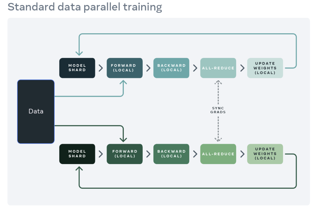
DDP (Distributed Data Parallel) was the initial step up from training with only a single GPU, and was an effort to address the data and model size growth, where multiple GPUs each housed their own copy of the same model. The gain here is that the data for each batch could be split and processed independently on each GPU, all at the same time,thus parallelizing the processing of the data set and increasing training speed by the increasing number of GPUs. The tradeoff is the need to communicate the gradients between each GPU to synchronize the models after the backward pass.

FSDP expands on scaling models by removing the redundancy of optimizer calculations and state storage, as well as gradient and memory storage of model parameters that are present in DDP (DDP = Distributed Data Parallel). This redundancy reduction, along with increased communication overlap where model parameter communication takes place at the same time as model computation, is what allows FSDP to train much larger models with the same resources as DDP.

A key point is that this efficiency also allows for AI models that are larger than a single GPU to be trained. The model size available for training is now increased to the aggregate memory of all GPUs, rather than the size of a single GPU. (And as a point of note, FSDP can go beyond aggregated GPU memory by leveraging CPU memory as well, though we will not directly cover this aspect here).

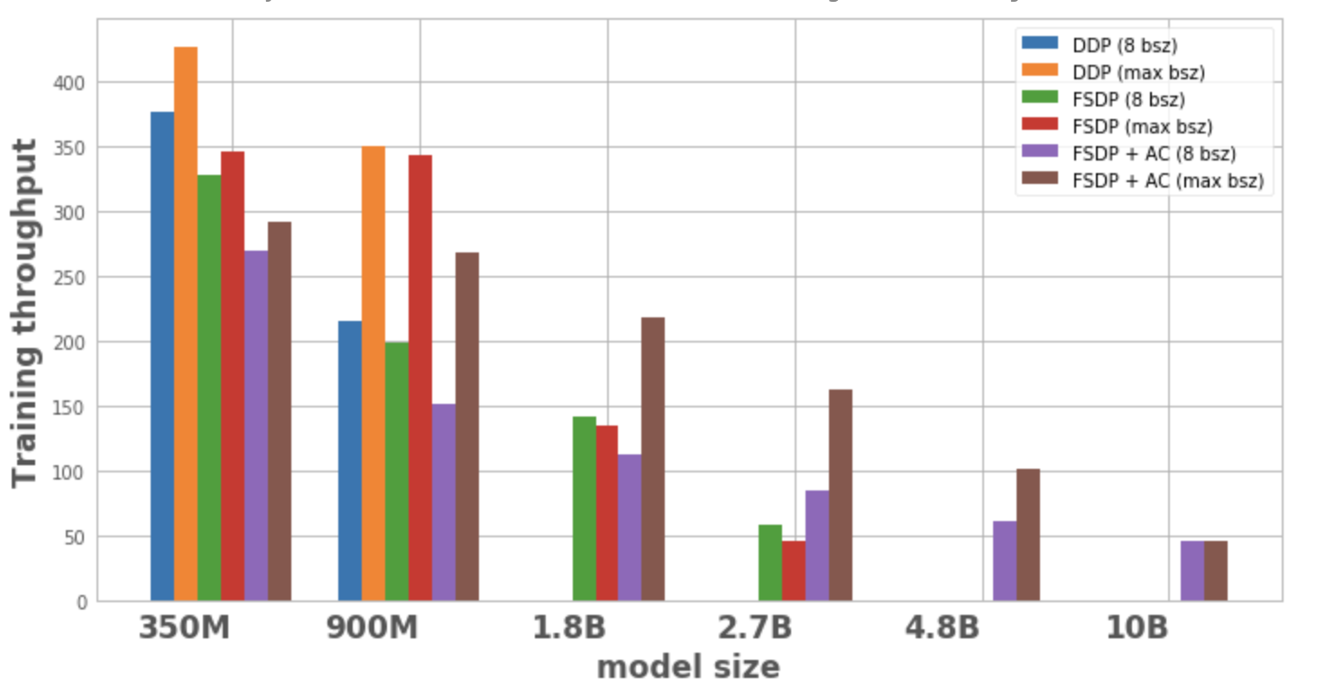
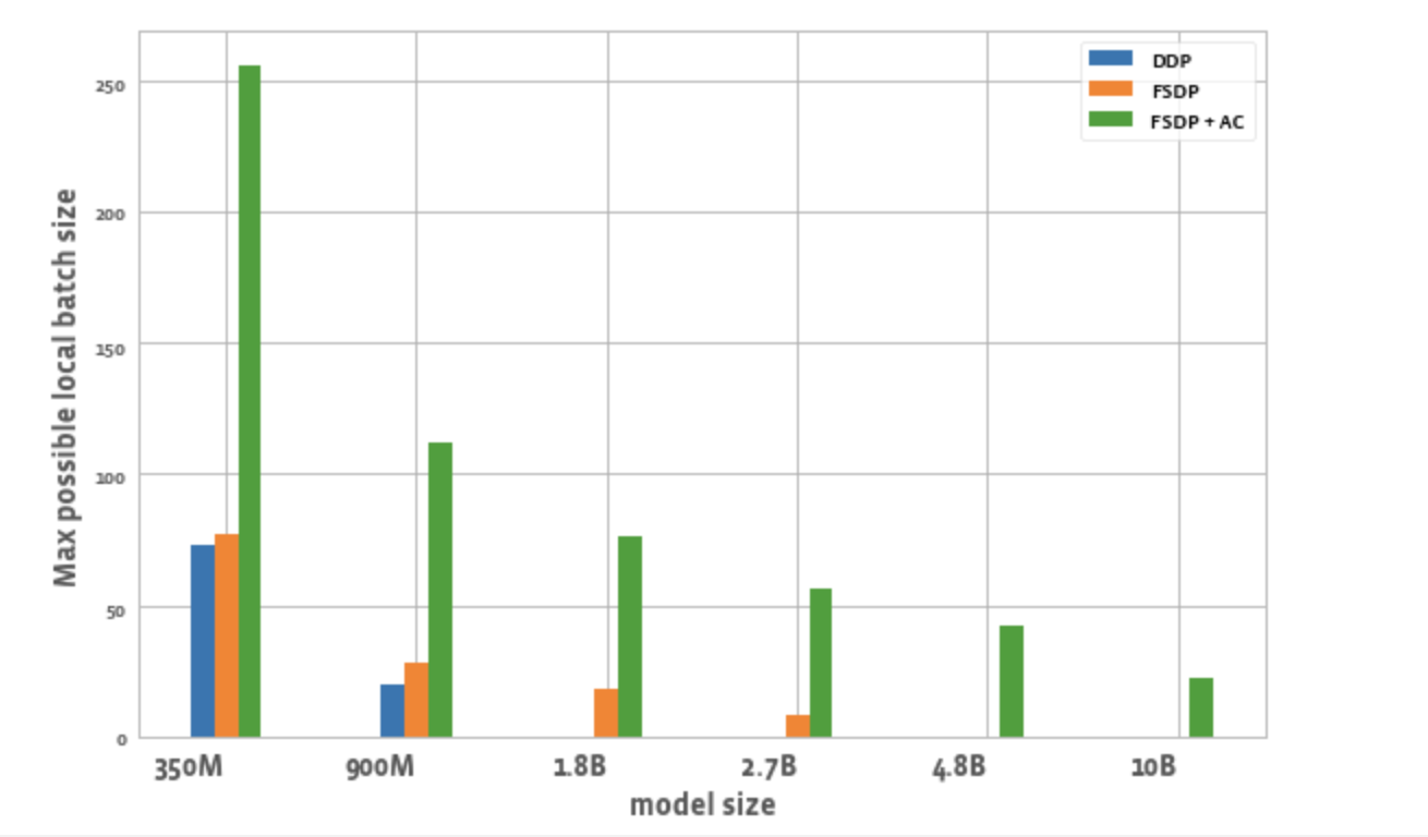
As discussed in a previous blog post, with DDP the largest model that we could train on 32, A100 gpus with 40 GB memory (4 nodes) was up to 3B parameters, and batch size of 128, with the help of activation checkpointing. By contrast, using FSDP we were able to train up to 81B model size, combining activation checkpointing, along with activation and parameter offloading. In another experiment, we benchmarked a 1T parameter model with FSDP using 512 gpus.

>>>>> gd2md-html alert: inline image link here (to images/image3.png). Store image on your image server and adjust path/filename/extension if necessary.
(Back to top)(Next alert)
>>>>>

For intuition on the parameter level workings of FSDP, below we show an animation detailing how the model parameters are sharded and communicated assuming a two GPU scenario and a simple 8 parameter model:

>>>>> gd2md-html alert: inline image link here (to images/image4.gif). Store image on your image server and adjust path/filename/extension if necessary.
(Back to top)(Next alert)
>>>>>

Above – the animations walk through the steps involved with the initial sharding of the model amongst ranks, and we start the all_gathers and forward pass.

>>>>> gd2md-html alert: inline image link here (to images/image5.gif). Store image on your image server and adjust path/filename/extension if necessary.
(Back to top)(Next alert)
>>>>>

We continue through the model with the forward pass. After each FSDP unit completes, non-locally owned params are dropped to free memory, and optionally activations can be checkpointed. This continues until we finish the forward pass and compute the loss.

>>>>> gd2md-html alert: inline image link here (to images/image6.gif). Store image on your image server and adjust path/filename/extension if necessary.
(Back to top)(Next alert)
>>>>>

_During the backward pass, another all_gather is used to load the parameters and the gradients are computed. These gradients are then reduce_scattered so that the local owners of each param can aggregate and prepare to update the weights. _

>>>>> gd2md-html alert: inline image link here (to images/image7.gif). Store image on your image server and adjust path/filename/extension if necessary.
(Back to top)(Next alert)
>>>>>

_Finally, each rank passes the summed gradients through the optimizer states and updates the weights to complete the mini-batch. _

With the model now distributed across the entire set of available GPUs, the logical question is how data moves through the model given this sharding of model parameters.

This is accomplished by FSDP coordinating with all GPUs to effectively share (communicate) the respective parts of the model. The model is decomposed into FSDP units and parameters within each unit are flattened and then sharded across all GPUs. Within each FSDP unit, GPU’s are assigned interleaving ownership of individual model parameters.

By interleaving, we mean the following – assuming 2 gpus with an id of 1 and 2, the FSDP unit ownership pattern would be [12121212], rather than a contiguous chunk of [111222].

During training, an all_gather is initiated and the locally owned model parameters within a FSDP unit are shared by the owner GPU with the other non-owners, when they need it, on a ‘just in time’ type basis. FSDP prefetches parameters to overlap all_gather communication with computation.

When those requested parameters arrive, the GPU uses the delivered parameters, in combination with the parameters it already owns, to create a fully populated FSDP unit. Thus there is a moment where each GPU hits peak memory usage while holding a fully populated FSDP unit.

It then processes the data through the FSDP unit, and drops the parameters it received from other GPU’s to free up memory for the next unit…the process continues over and over proceeding through the entire model to complete the forward pass. The process is then repeated (in general) for the backward pass.
(note – this is a simplified version for understanding..there is additional complexity but this should help construct a basic mental model of the FSDP process).

This eliminates much of the memory redundancy present in DDP, but imposes the cost of higher amounts of network communication to shuttle these requested parameters back and forth amongst all the GPUs. ** Overlapping the communication timing with the computation taking place is the basis of many of the performance improvements we’ll discuss in this series.** The key gains are frequently based on the fact that communication can often take place at the same time as computation. As you can surmise, having high communication speed is vital for FSDP performance.

How do I optimize my training with FSDP?

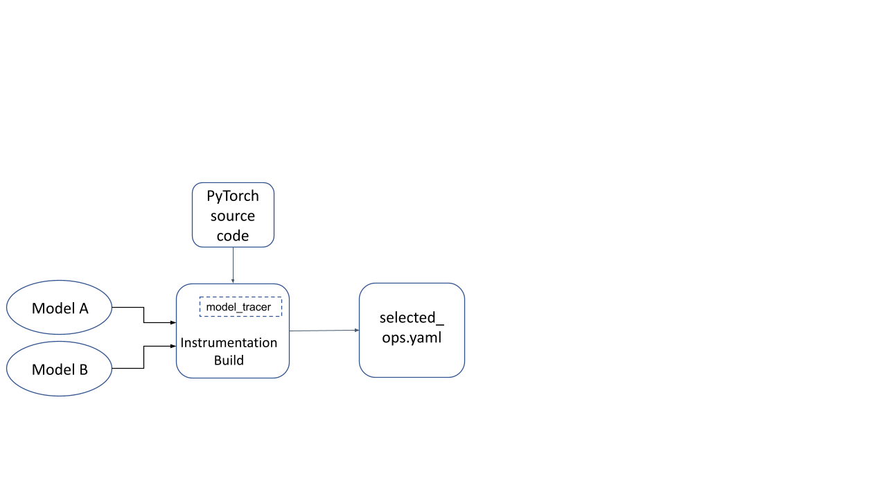
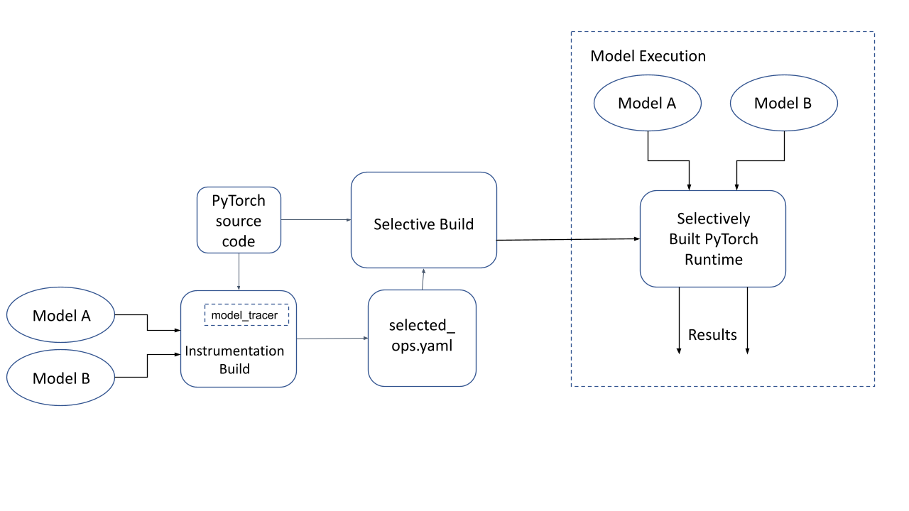
There are four main performance improvements we will cover – the transformer wrapper, activation checkpointing, mixed precision, and selecting the proper sharding strategy. The flowchart below will help as a checklist for tuning options that we will discuss in this post.

>>>>> gd2md-html alert: inline image link here (to images/image8.png). Store image on your image server and adjust path/filename/extension if necessary.
(Back to top)(Next alert)
>>>>>

Wrapping policy – for transformers, use Transformer wrapping policy

The first performance optimization is leveraging the FSDP transformer wrapper for transformer models.

One of the pre-defined wrapping policy is size_based_autowrap_policy. With size_based_autowrap_policy, FSDP will traverse the module structure from bottom to top, a new FSDP unit will be created once the current unit has at least the ‘min_num_params’ specified within the size policy (this defaults to 1e8, or 100M). If the module can not be created as an FSDP unit, FSDP will continue to check its parent module. This size based wrapping policy may not be ideal for some model structures, PyTorch distributed team is actively working on a new default wrapping policy in the next release which is based on size and also module execution order, users can simply tune the size and achieve the optimized performance.

In the current release, you can greatly improve your performance when running Transformer models by using the ‘transformer wrapper’. You will need to provide the appropriate layer class for your model. Here, layer class is the class that houses the Multi-Head Attention and Feed Forward Network.

FSDP will then form the FSDP units around the layer class rather than arbitrary breaks based on parameter size. By sharding the model around layer classes that are uniformly repeated within the transformer, FSDP can create uniform FSDP units that better balance the overlap of computation and communication. By contrast, size based wrapping can produce very uneven or skewed shards for models, which then have uneven matching of compute vs communication overlap. As discussed earlier, the main driver of FSDP high performance is the overlap of communication and computation, and hence why the Transformer wrapper provides improved performance. Note that the Transformer wrapper can also be used for non-transformer models if these models have a list of uniform layers.

Let’s compare the performance difference on a T5, 3B parameter model when running under the default wrapper and the transformer wrapper.

For default wrapping, we don’t need to take any action – we simply pass the model to FSDP as shown:

model = FSDP(
      model,
      device_id=torch.cuda.current_device(),
  )

In this case FSDP will simply wrap the whole model in a single FSDP unit.

Running on an NVIDIA A100-SXM4–40GB with 8 GPUs, we are able to reach 2.3 TFlops and 95% GPU memory utilization with a batch size of 14.

However, since T5 is a transformer model, we are better served to leverage the transformer wrapper for this model.

To use that, we need to isolate the layer class for the transformer, and then pass it in to create our transformer wrapper.

from transformers.models.t5.modeling_t5 import T5Block

And now we can create our Transformer wrapper:

transformer_auto_wrapper_policy = functools.partial(
        transformer_auto_wrap_policy,
        transformer_layer_cls={
            T5Block,  # < ---- Your Transformer layer class
        },
    )

With our model aware wrapper ready, we can initialize FSDP:

# invoke FSDP with your transformer wrapper policy:
model = FSDP(
        model,
        auto_wrap_policy=transformer_auto_wrapper_policy,
        device_id=torch.cuda.current_device(),  # streaming init
    )

Running this wrapped model, we can see some substantial performance gains.
We can fit nearly double the batch size, going to 28, and with better memory and communication efficiency, we see a TFlops increase to 5.07 from 2.3.

Thus, we’ve increased our training throughput by over 200% (2.19x) due to providing greater model info to FSDP! The transformer wrapping policy results in more fine-grained and balanced FSDP units each holding a layer class, which leads to a more effective communication-computation overlap.

>>>>> gd2md-html alert: inline image link here (to images/image9.png). Store image on your image server and adjust path/filename/extension if necessary.
(Back to top)(Next alert)
>>>>>

Above: Graphical comparison of TFlops based on wrapper type

If you are training a Transformer model, it pays to configure your training with FSDP using the transformer wrapper. For more information on how to isolate your layer class, please see our in depth video on Transformer wrapping here, where we walk through a number of transformers showing where the layer class can be found.

Mixed precision -_ use BF16 if you have an Ampere architecture GPU_

FSDP supports a flexible mixed precision policy that gives you granular control over parameters, gradients and buffer data types. This lets you easily leverage BFloat16 or FP16 to increase your training speed by up to 70%.

*Note that BFloat 16 is only available on Ampere type GPUs. On AWS this is available with p4dn and g5 instances.

By way of comparison, we can show a 77% speed improvement when comparing fully tuned BFloat16 vs FP32 on an 8B DeepVit model.

>>>>> gd2md-html alert: inline image link here (to images/image10.png). Store image on your image server and adjust path/filename/extension if necessary.
(Back to top)(Next alert)
>>>>>

We have obtained even greater acceleration using BFloat16 in fine-tuning a 3B HuggingFace T5 model as shown in the figures below. We observed that because of the lower precision the validation loss of BFloat16 is slightly behind in the first few epochs, but it is able to catch up and results in the same final accuracy as FP32.

>>>>> gd2md-html alert: inline image link here (to images/image11.png). Store image on your image server and adjust path/filename/extension if necessary.
(Back to top)(Next alert)
>>>>>

To use mixed precision, we create a policy with our desired data types, and pass it in during the FSDP initialization.
To create our policy, we need to import the MixedPrecision class, and then define our custom policy using our customized class:

from torch.distributed.fsdp import MixedPrecision

bfSixteen = MixedPrecision(
   param_dtype=torch.bfloat16,
   # Gradient communication precision.
   reduce_dtype=torch.bfloat16,
   # Buffer precision.
   buffer_dtype=torch.bfloat16,
)

model = FSDP(
       model,
       auto_wrap_policy=transformer_auto_wrapper_policy,
       mixed_precision=bfloatPolicy)

You can mix and match the precision for parameters, gradients and buffers as you prefer:

comboPolicy = MixedPrecision(
        # Param precision
        param_dtype=torch.bfloat16,
        # Gradient communication precision.
        reduce_dtype=torch.float32,
        # Buffer precision.
        buffer_dtype=torch.float32,
    )

For training with FP16, you will need to also use the ShardedGradScaler, which we will cover in subsequent posts. For BFloat16, it is a drop-in replacement.

AnyPrecision Optimizer – _going beyond mixed precision with full BF16 training _

Mixed precision training, both in FSDP and elsewhere, maintains the working weights in the reduced datatype (BF16 or FP16) while keeping the master weights in full FP32. The reason for the master weights in FP32 is that running in pure BF16 will result in ‘weight stagnation’, where very small weight updates are lost due to the lower precision, and the accuracy flatlines over time while FP32 weights can continue to improve from these small updates.

In order to resolve this dilemma, we can use the new AnyPrecision optimizer available in TorchDistX (Torch Distributed Experimental) that allows you to successfully train and keep the master weights in pure BF16 instead of FP32. In addition, unlike the typical storage of optimizer states in FP32, AnyPrecision is able to maintain states in pure BF16 as well.

AnyPrecision enables pure BF16 training by maintaining an extra buffer that tracks the precision lost during the weight updates and re-applies that during the next update…effectively resolving the weight stagnation issue without requiring FP32.

As a comparison of the throughput gains available with pure BF16 training using AnyPrecision, we ran experiments using FSDP with the T5 11B model with regular FP32 training, Mixed Precision training with BF16, and pure BF16 training using the AnyPrecision optimizer on 3 nodes with A100 gpus as mentioned previously.

>>>>> gd2md-html alert: inline image link here (to images/image12.png). Store image on your image server and adjust path/filename/extension if necessary.
(Back to top)(Next alert)
>>>>>

As shown above, training with AnyPrecision and pure BF16 resulted in 2x the throughput vs Mixed Precision, and over 20x improvement vs FP32.

The potential tradeoff is the impact on final accuracy – in the cases we tested, the accuracy was equal or better than FP32 due to a regularization effect from the slightly reduced precision, but your results may vary.

AnyPrecision optimizer is available for you to test with here, and is a drop in replacement for AdamW optimizer.

Activation checkpointing – increasing throughput by trading compute for memory

>>>>> gd2md-html alert: inline image link here (to images/image13.png). Store image on your image server and adjust path/filename/extension if necessary.
(Back to top)(Next alert)
>>>>>

FSDP supports activation checkpointing once the model has been sharded, and makes it easy to implement. The graph above shows ~4x throughput improvement using activation checkpointing.

Activation checkpointing is where the intermediate activations are freed during the forward pass, and a checkpoint is left as a placeholder. This generally increases available GPU memory by over 30%.

The tradeoff is that during the backward pass, these previously removed intermediate activations must be re-calculated again using information in the checkpoint (duplicate compute), but by leveraging the increased GPU memory, one can increase the batch size such that the net throughput can increase substantially.

# verify we have FSDP activation support ready by importing:
from torch.distributed.algorithms._checkpoint.checkpoint_wrapper import (
   checkpoint_wrapper,
   CheckpointImpl,
   apply_activation_checkpointing_wrapper,
)

The steps required to implement activation checkpointing is to first import the FSDP checkpointing functions. We need declare our checkpointer wrapper type which is non-reentrant and create a check function to identify which layer to wrap as follows

non_reentrant_wrapper = partial(
    checkpoint_wrapper,
    offload_to_cpu=False,
    checkpoint_impl=CheckpointImpl.NO_REENTRANT,
)

check_fn = lambda submodule: isinstance(submodule, T5Block)

apply_activation_checkpointing_wrapper(
       model, checkpoint_wrapper_fn=non_reentrant_wrapper, check_fn=check_fn
   )

Important note – this must be run after the model has been initialized with FSDP.

However, hopefully you’ve seen how some initial tuning with FSDP options can have a large impact on your training performance.

With that, we turn our attention from how to scale within FSDP, to how to scale your server hardware for FSDP using AWS.

Large Scale Training with FSDP on AWS – For multi-node prioritize high speed network

AWS provides several services that can be used to run distributed training with FSDP:
Amazon EC2 Accelerated Computing instances, AWS ParallelCluster, and Amazon Sagemaker.

In this series of blog posts, we used Amazon EC2 p4d instances in a single-instance multi-GPU configuration and in a multi-instance configuration using AWS ParallelCluster and SageMaker in order to run our training jobs.

Here, we’ll focus specifically on AWS parallel cluster and provide an overview of how to utilize it for training purposes.

AWS ParallelCluster Setup

>>>>> gd2md-html alert: inline image link here (to images/image14.png). Store image on your image server and adjust path/filename/extension if necessary.
(Back to top)(Next alert)
>>>>>

Workflow on Clusters

The high level idea is to have a cluster that has a head node which controls the compute nodes. The actual training job runs on the compute nodes. Overall steps to run a training job on a cluster are as follows:

1. Set up an AWS ParallelCuster (we discuss below)
2. Connect to the head node, and import the training code/ setup the environment.
3. Pull the data and place it in a shared folder that compute nodes can access (FSx Lustre drive).
4. Run the training job using a job scheduler (in this case Slurm).

Setup AWS ParallelCuster

To setup AWS** **ParallelCluster,

1. Deploy a network stack. This step is optional since you could use your account default VPC and let AWS ParallelCluster create your subnets and security groups. However, we prefer to compartmentalize our desired network infrastructure and do this deployment via a CloudFormation stack.

   Since we deploy a public and a private subnet, we want to create them into an Availability Zone that contains our target instances, in this case p4d. We consult their availability in the region we use (us-east-1) through the following AWS CLI command:

   aws ec2 describe-instance-type-offerings --location-type availability-zone --filters Name=instance-type,Values=p4d.24xlarge --region us-east-1 --output table

   We see three availability zones containing p4d instances, we pick one of them (us-east-1c, yours may be different) when deploying our network stack. This can be done with the AWS Console or the AWS CLI. In our case we use the latter as follows

   ` aws cloudformation create-stack –stack-name VPC-Large-Scale –capabilities CAPABILITY_IAM –template-body file://VPC-Large-Scale.yaml –parameters ParameterKey=SubnetsAZ,ParameterValue=us-east-1c`

   CloudFormation will deploy our new VPC, subnets, security groups and endpoints on our behalf. Once done, you can retrieve the IDs of the public and private subnets by querying the stack outputs and the values PublicSubnet and PrivateSubnet.

   For example, using the AWS CLI for the private subnet:

   aws cloudformation describe-stacks --stack-name VPC-Large-Scale --query "Stacks[0].Outputs[?OutputKey=='PrivateSubnet'].OutputValue" --output text

2. Create ParallelCluster, The cluster configuration file specifies the resources for our cluster. These resources include instance type for Head node, compute nodes, access to S3 buckets, shared storage where our data will be located. We will use Amazon FSx for Lustre that offers a fully managed shared storage service with Lustre.

   Here is an example of a cluster configuration file. We can use AWs ParallelCluster CLI to create the cluster. Please note that the private and public subnet IDs will need to be replaced by the ones you retrieved earlier. You will be able to control the cluster using the AWS ParallelCluster CLI to start, stop, pause, etc.

   pcluster create-cluster --cluster-name my-hpc-cluster --cluster-configuration cluster.yaml
   

3. SSH to Head node – once the cluster is ready, we can connect to the Head node using the SSH protocol, pull our training code with and place the data in the shared storage specified in the cluster configuration file.

   pcluster ssh --cluster-name cluster -i your-key_pair
   

4. Launch the training job – now that we have the data and training code, we can launch the slurm job for training. Here is an example of a slurm script to launch the job using torchrun.

More details on how to set up the cluster is out of the scope of this post, however we will have a separate post on it.

What’s next?

With this post we provided a high level overview of FSDP and how it efficiently scales distributed AI training. The flowchart included will help provide a checklist for you to review tuning options discussed such as the transformer wrapper and activation checkpointing.
In the next posts, we will continue with the T5 model and go deeper into each of the topics above, specifically with sharding strategy and other optimizations to provide more insight and details. For now, a good reference for the sharding strategy is in our video tutorial here:

If you have questions or find an issue, please find the authors Less, Hamid and Geeta or open an issue on PyTorch github.

Special thanks to:

Pytorch Distributed team, Shen Li, Rohan Varma, Yanli Zhao, Andrew Gu, Anjali Sridhar, Ana Simoes, Pierre-Yves Aquilanti, Sundar Ranganathan, and the broader AWS team for supporting us with providing infrastructure and technical support for running the large scale experiments.

Resources:

FSDP video series

Getting started with FSDP

Advanced tutorial on FSDP

API documentation

Read More

TorchVision is extending its Transforms API! Here is what’s new:

• You can use them not only for Image Classification but also for Object Detection, Instance & Semantic Segmentation and Video Classification.
• You can import directly from TorchVision several SoTA data-augmentations such as MixUp, CutMix, Large Scale Jitter and SimpleCopyPaste.
• You can use new functional transforms for transforming Videos, Bounding Boxes and Segmentation Masks.

The interface remains the same to assist the migration and adoption. The new API is currently in Prototype and we would love to get early feedback from you to improve its functionality. Please reach out to us if you have any questions or suggestions.

Limitations of current Transforms

The stable Transforms API of TorchVision (aka V1) only supports single images. As a result it can only be used for classification tasks:

from torchvision import transforms
trans = transforms.Compose([
   transforms.ColorJitter(contrast=0.5),
   transforms.RandomRotation(30),
   transforms.CenterCrop(480),
])
imgs = trans(imgs)

The above approach doesn’t support Object Detection, Segmentation or Classification transforms that require the use of Labels (such as MixUp & CutMix). This limitation made any non-classification Computer Vision tasks second-class citizens as one couldn’t use the Transforms API to perform the necessary augmentations. Historically this made it difficult to train high-accuracy models using TorchVision’s primitives and thus our Model Zoo lagged by several points from SoTA.

To circumvent this limitation, TorchVision offered custom implementations in its reference scripts that show-cased how one could perform augmentations in each task. Though this practice enabled us to train high accuracy classification, object detection & segmentation models, it was a hacky approach which made those transforms impossible to import from the TorchVision binary.

The new Transforms API

The Transforms V2 API supports videos, bounding boxes, labels and segmentation masks meaning that it offers native support for many Computer Vision tasks. The new solution is a drop-in replacement:

from torchvision.prototype import transforms
# Exactly the same interface as V1:
trans = transforms.Compose([
    transforms.ColorJitter(contrast=0.5),
    transforms.RandomRotation(30),
    transforms.CenterCrop(480),
])
imgs, bboxes, labels = trans(imgs, bboxes, labels)

The new Transform Classes can receive any arbitrary number of inputs without enforcing specific order or structure:

# Already supported:
trans(imgs)  # Image Classification
trans(videos)  # Video Tasks
trans(imgs_or_videos, labels)  # MixUp/CutMix-style Transforms
trans(imgs, bboxes, labels)  # Object Detection
trans(imgs, bboxes, masks, labels)  # Instance Segmentation
trans(imgs, masks)  # Semantic Segmentation
trans({"image": imgs, "box": bboxes, "tag": labels})  # Arbitrary Structure
# Future support:
trans(imgs, bboxes, labels, keypoints)  # Keypoint Detection
trans(stereo_images, disparities, masks)  # Depth Perception
trans(image1, image2, optical_flows, masks)  # Optical Flow

The Transform Classes make sure that they apply the same random transforms to all the inputs to ensure consistent results.

The functional API has been updated to support all necessary signal processing kernels (resizing, cropping, affine transforms, padding etc) for all inputs:

from torchvision.prototype.transforms import functional as F
# High-level dispatcher, accepts any supported input type, fully BC
F.resize(inpt, resize=[224, 224])
# Image tensor kernel
F.resize_image_tensor(img_tensor, resize=[224, 224], antialias=True)
# PIL image kernel
F.resize_image_pil(img_pil, resize=[224, 224], interpolation=BILINEAR)
# Video kernel
F.resize_video(video, resize=[224, 224], antialias=True)
# Mask kernel
F.resize_mask(mask, resize=[224, 224])
# Bounding box kernel
F.resize_bounding_box(bbox, resize=[224, 224], spatial_size=[256, 256])

The API uses Tensor subclassing to wrap input, attach useful meta-data and dispatch to the right kernel. Once the Datasets V2 work is complete, which makes use of TorchData’s Data Pipes, the manual wrapping of input won’t be necessary. For now, users can manually wrap the input by:

from torchvision.prototype import features
imgs = features.Image(images, color_space=ColorSpace.RGB)
vids = features.Video(videos, color_space=ColorSpace.RGB)
masks = features.Mask(target["masks"])
bboxes = features.BoundingBox(target["boxes"], format=BoundingBoxFormat.XYXY, spatial_size=imgs.spatial_size)
labels = features.Label(target["labels"], categories=["dog", "cat"])

In addition to the new API, we now provide importable implementations for several data augmentations that are used in SoTA research such as MixUp, CutMix, Large Scale Jitter, SimpleCopyPaste, AutoAugmentation methods and several new Geometric, Colour and Type Conversion transforms.

The API continues to support both PIL and Tensor backends for Images, single or batched input and maintains JIT-scriptability on the functional API. It allows deferring the casting of images from uint8 to float which can lead to performance benefits. It is currently available in the prototype area of TorchVision and can be imported from the nightly builds. The new API has been verified to achieve the same accuracy as the previous implementation.

Current Limitations

Though the functional API (kernels) remain JIT-scriptable and fully-BC, the Transform Classes, though they offer the same interface, can’t be scripted. This is because they use Tensor Subclassing and receive arbitrary number of inputs which are not supported by JIT. We are currently working to reduce the dispatching overhead of the new API and to improve the speed of existing kernels.

An end-to-end example

Here is an example of the new API using the following image. It works both with PIL images and Tensors:

import PIL
from torchvision import io, utils
from torchvision.prototype import features, transforms as T
from torchvision.prototype.transforms import functional as F
# Defining and wrapping input to appropriate Tensor Subclasses
path = "COCO_val2014_000000418825.jpg"
img = features.Image(io.read_image(path), color_space=features.ColorSpace.RGB)
# img = PIL.Image.open(path)
bboxes = features.BoundingBox(
    [[2, 0, 206, 253], [396, 92, 479, 241], [328, 253, 417, 332],
     [148, 68, 256, 182], [93, 158, 170, 260], [432, 0, 438, 26],
     [422, 0, 480, 25], [419, 39, 424, 52], [448, 37, 456, 62],
     [435, 43, 437, 50], [461, 36, 469, 63], [461, 75, 469, 94],
     [469, 36, 480, 64], [440, 37, 446, 56], [398, 233, 480, 304],
     [452, 39, 463, 63], [424, 38, 429, 50]],
    format=features.BoundingBoxFormat.XYXY,
    spatial_size=F.get_spatial_size(img),
)
labels = features.Label([59, 58, 50, 64, 76, 74, 74, 74, 74, 74, 74, 74, 74, 74, 50, 74, 74])
# Defining and applying Transforms V2
trans = T.Compose(
    [
        T.ColorJitter(contrast=0.5),
        T.RandomRotation(30),
        T.CenterCrop(480),
    ]
)
img, bboxes, labels = trans(img, bboxes, labels)
# Visualizing results
viz = utils.draw_bounding_boxes(F.to_image_tensor(img), boxes=bboxes)
F.to_pil_image(viz).show()

Development milestones and future work

Here is where we are in development:

• Design API
• Write Kernels for transforming Videos, Bounding Boxes, Masks and Labels
• Rewrite all existing Transform Classes (stable + references) on the new API:
  • Image Classification
  • Video Classification
  • Object Detection
  • Instance Segmentation
  • Semantic Segmentation
• Verify the accuracy of the new API for all supported Tasks and Backends
• Speed Benchmarks and Performance Optimizations (in progress – planned for Dec)
• Graduate from Prototype (planned for Q1)
• Add support of Depth Perception, Keypoint Detection, Optical Flow and more (future)

We are currently in the process of Benchmarking each Transform Class and Functional Kernel in order to measure and improve their performance. The scope includes optimizing existing kernels which will be adopted from V1. Early findings indicate that some improvements might need to be upstreamed on the C++ kernels of PyTorch Core. Our plan is to continue iterating throughout Q4 to improve the speed performance of the new API and enhance it with additional SoTA transforms with the help of the community.

We would love to get early feedback from you to improve its functionality. Please reach out to us if you have any questions or suggestions.

Read More

Summary

We are bringing a number of improvements to the current PyTorch libraries, alongside the PyTorch 1.13 release. These updates demonstrate our focus on developing common and extensible APIs across all domains to make it easier for our community to build ecosystem projects on PyTorch.

Along with 1.13, we are releasing updates to the PyTorch Libraries, please find them below.

TorchAudio

(Beta) Hybrid Demucs Model and Pipeline

Hybrid Demucs is a music source separation model that uses both spectrogram and time domain features. It has demonstrated state-of-the-art performance in the Sony^® Music DeMixing Challenge. (citation: https://arxiv.org/abs/2111.03600)

The TorchAudio v0.13 release includes the following features

• MUSDB_HQ Dataset, which is used in Hybrid Demucs training (docs)
• Hybrid Demucs model architecture (docs)
• Three factory functions suitable for different sample rate ranges
• Pre-trained pipelines (docs)
• SDR Results of pre-trained pipelines on MUSDB_HQ test set
• Tutorial that steps through music source separation using the pretrained pipeline (docs)

* Trained on the training data of MUSDB-HQ dataset.
** Trained on both training and test sets of MUSDB-HQ and 150 extra songs from an internal database that were specifically produced for Meta.

from torchaudio.pipelines import HDEMUCS_HIGH_MUSDB_PLUS

bundle = HDEMUCS_HIGH_MUSDB_PLUS
model = bundle.get_model()
sources_list = model.sources

mixture, samplerate = torchaudio.load(“song.wav”)
sources = model(mixture)
audios = dict(zip(sources_list, sources)

Special thanks to Alexandre Defossez for the guidance.

(Beta) Datasets and Metadata Mode for SUPERB Benchmark

TorchAudio adds support for various audio-related datasets used in downstream tasks for benchmarking self-supervised learning models. With the addition of several new datasets, there is now support for the downstream tasks in version 1 of the SUPERB benchmark, which can be found in the s3prl repository.

For these datasets, we also add metadata support through a get_metadata function, enabling faster dataset iteration or preprocessing without the need to load waveforms. The function returns the same features as __getitem__, except it returns the relative waveform path rather than the loaded waveform.

Datasets with metadata functionality

• LIBRISPEECH (docs)
• LibriMix (docs)
• QUESST14 (docs)
• SPEECHCOMMANDS (docs)
• (new) FluentSpeechCommands (docs)
• (new) Snips (docs)
• (new) IEMOCAP (docs)
• (new) VoxCeleb1 (Identification, Verification)

(Beta) Custom Language Model support in CTC Beam Search Decoding

TorchAudio released a CTC beam search decoder in release 0.12, with KenLM language model support. This release, there is added functionality for creating custom Python language models that are compatible with the decoder, using the torchaudio.models.decoder.CTCDecoderLM wrapper.

For more information on using a custom language model, please refer to the documentation and tutorial.

(Beta) StreamWriter

torchaudio.io.StreamWriter is a class for encoding media including audio and video. This can handle a wide variety of codecs, chunk-by-chunk encoding and GPU encoding.

writer = StreamWriter("example.mp4")
writer.add_audio_stream(
    sample_rate=16_000,
    num_channels=2,
)
writer.add_video_stream(
    frame_rate=30,
    height=96,
    width=128,
    format="rgb24",
)
with writer.open():
    writer.write_audio_chunk(0, audio)
    writer.write_video_chunk(1, video)

For more information, refer to the documentation and the following tutorials

• StreamWriter Basic Usage
• StreamWriter Advanced Usage
• Hardware-Accelerated Video Decoding and Encoding

TorchData

For a complete list of changes and new features, please visit our repository’s 0.5.0 release note.

(Prototype) DataLoader2

DataLoader2 was introduced in the last release to execute DataPipe graph, with support for dynamic sharding for multi-process/distributed data loading, multiple backend ReadingServices, and DataPipe graph in-place modification (e.g. shuffle control).

In this release, we further consolidated the API for DataLoader2 and a detailed documentation is now available here. We continue to welcome early adopters and feedback, as well as potential contributors. If you are interested in trying it out, we encourage you to install the nightly version of TorchData.

(Beta) Data Loading from Cloud Service Providers

We extended our support to load data from additional cloud storage providers via DataPipes, now covering AWS, Google Cloud Storage, and Azure. A tutorial is also available. We are open to feedback and feature requests.

We also performed a simple benchmark, comparing the performance of data loading from AWS S3 and attached volume on an AWS EC2 instance. The results are visible here.

torch::deploy (Beta)

torch::deploy is now in Beta! torch::deploy is a C++ library for Linux based operating systems that allows you to run multiple Python interpreters in a single process. You can run your existing eager PyTorch models without any changes for production inference use cases. Highlights include:

• Existing models work out of the box–no need to modify your python code to support tracing.
• Full support for your existing Python environment including C extensions.
• No need to cross process boundaries to load balance in multi-GPU serving environments.
• Model weight can be shared between multiple Python interpreters.
• A vastly improved installation and setup process.

torch::deploy::InterpreterManager manager(4);

// access one of the 4 interpreters
auto I = manager.acquireOne();

// run infer from your_model.py
I.global("your_model", "infer")({at::randn({10, 240, 320})});

Learn more here.

(Beta) CUDA/ROCm/CPU Backends

torch::deploy now links against standard PyTorch Python distributions so all accelerators that PyTorch core supports such as CUDA and AMD/HIP work out of the box.

• Can install any device variant of PyTorch via pip/conda like normal.
• https://pytorch.org/get-started/locally/

(Prototype) aarch64/arm64 support

torch::deploy now has basic support for aarch64 Linux systems.

• We’re looking to gather feedback on it and learn more about arm use cases for eager PyTorch models.
• Learn more / share your use case at https://github.com/pytorch/multipy/issues/64

TorchEval

(Prototype) Introducing Native Metrics Support for PyTorch

TorchEval is a library built for users who want highly performant implementations of common metrics to evaluate machine learning models. It also provides an easy to use interface for building custom metrics with the same toolkit. Building your metrics with TorchEval makes running distributed training loops with torch.distributed a breeze.

Learn more with our docs, see our examples, or check out our GitHub repo.

TorchMultimodal Release (Beta)

Please watch for upcoming blogs in early November that will introduce TorchMultimodal, a PyTorch domain library for training SoTA multi-task multimodal models at scale, in more details; in the meantime, play around with the library and models through our tutorial.

TorchRec

(Prototype) Simplified Optimizer Fusion APIs

We’ve provided a simplified and more intuitive API for setting fused optimizer settings via apply_optimizer_in_backward. This new approach enables the ability to specify optimizer settings on a per-parameter basis and sharded modules will configure FBGEMM’s TableBatchedEmbedding modules accordingly. Additionally, this now let’s TorchRec’s planner account for optimizer memory usage. This should alleviate reports of sharding jobs OOMing after using Adam using a plan generated from planner.

(Prototype) Simplified Sharding APIs

We’re introducing the shard API, which now allows you to shard only the embedding modules within a model, and provides an alternative to the current main entry point – DistributedModelParallel. This lets you have a finer grained control over the rest of the model, which can be useful for customized parallelization logic, and inference use cases (which may not require any parallelization on the dense layers). We’re also introducing construct_module_sharding_plan, providing a simpler interface to the TorchRec sharder.

(Beta) Quantized Comms

Applying quantization or mixed precision to tensors in a collective call during model parallel training greatly improves training efficiency, with little to no effect on model quality. TorchRec now integrates with the quantized comms library provided by FBGEMM GPU and provides an interface to construct encoders and decoders (codecs) that surround the all_to_all, and reduce_scatter collective calls in the output_dist of a sharded module. We also allow you to construct your own codecs to apply to your sharded module. The codces provided by FBGEMM allow FP16, BF16, FP8, and INT8 compressions, and you may use different quantizations for the forward pass and backward pass.

TorchSnapshot (Beta)

Along with PyTorch 1.13, we are releasing the beta version of TorchSnapshot, which is a performant, memory-efficient checkpointing library for PyTorch applications, designed with large, complex distributed workloads in mind. Highlights include:

• Performance: TorchSnapshot provides a fast checkpointing implementation employing various optimizations, including zero-copy serialization for most tensor types, overlapped device-to-host copy and storage I/O, parallelized storage I/O
• Memory Use: TorchSnapshot’s memory usage adapts to the host’s available resources, greatly reducing the chance of out-of-memory issues when saving and loading checkpoints
• Usability: Simple APIs that are consistent between distributed and non-distributed workloads

Learn more with our tutorial.

TorchVision

We are happy to introduce torchvision v0.14 (release note). This version introduces a new model registration API to help users retrieving and listing models and weights. It also includes new image and video classification models such as MViT, S3D, Swin Transformer V2, and MaxViT. Last but not least, we also have new primitives and augmentation such as PolynomicalLR scheduler and SimpleCopyPaste.

(Beta) Model Registration API

Following up on the multi-weight support API that was released on the previous version, we have added a new model registration API to help users retrieve models and weights. There are now 4 new methods under the torchvision.models module: get_model, get_model_weights, get_weight, and list_models. Here are examples of how we can use them:

import torchvision
from torchvision.models import get_model, get_model_weights, list_models


max_params = 5000000

tiny_models = []
for model_name in list_models(module=torchvision.models):
    weights_enum = get_model_weights(model_name)
    if len([w for w in weights_enum if w.meta["num_params"] <= max_params]) > 0:
        tiny_models.append(model_name)

print(tiny_models)
# ['mnasnet0_5', 'mnasnet0_75', 'mnasnet1_0', 'mobilenet_v2', ...]

model = get_model(tiny_models[0], weights="DEFAULT")
print(sum(x.numel() for x in model.state_dict().values()))
# 2239188

(Beta) New Video Classification Models

We added two new video classification models, MViT and S3D. MViT is a state of the art video classification transformer model which has 80.757% accuracy on the Kinetics400 dataset, while S3D is a relatively small model with good accuracy for its size. These models can be used as follows:

import torch
from torchvision.models.video import *

video = torch.rand(3, 32, 800, 600)
model = mvit_v2_s(weights="DEFAULT")
# model = s3d(weights="DEFAULT")
model.eval()
prediction = model(images)

Here is the table showing the accuracy of the new video classification models tested in the Kinetics400 dataset.

We would like to thank Haoqi Fan, Yanghao Li, Christoph Feichtenhofer and Wan-Yen Lo for their work on PyTorchVideo and their support during the development of the MViT model. We would like to thank Sophia Zhi for her contribution implementing the S3D model in torchvision.

(Stable) New Architecture and Model Variants

For Classification Models, we’ve added the Swin Transformer V2 architecture along with pre-trained weights for its tiny/small/base variants. In addition, we have added support for the MaxViT transformer. Here is an example on how to use the models:

import torch
from torchvision.models import *

image = torch.rand(1, 3, 224, 224)
model = swin_v2_t(weights="DEFAULT").eval()
# model = maxvit_t(weights="DEFAULT").eval()
prediction = model(image)

Here is the table showing the accuracy of the models tested on ImageNet1K dataset.

We would like to thank Ren Pang and Teodor Poncu for contributing the 2 models to torchvision.

(Stable) New Primitives & Augmentations

In this release we’ve added the SimpleCopyPaste augmentation in our reference scripts and we up-streamed the PolynomialLR scheduler to PyTorch Core. We would like to thank Lezwon Castelino and Federico Pozzi for their contributions. We are continuing our efforts to modernize TorchVision by adding more SoTA primitives, Augmentations and architectures with the help of our community. If you are interested in contributing, have a look at the following issue.

Torch-TensorRT

(Prototype) TensorRT with FX2TRT frontend

Torch-TensorRT is the PyTorch integration for TensorRT, providing high performance inference on NVIDIA GPUs. Torch-TRT allows for optimizing models directly in PyTorch for deployment providing up to 6x performance improvement.

Torch-TRT is an AoT compiler which ingests an nn.Module or TorchScript module, optimizes compatible subgraphs in TensorRT & leaves the rest to run in PyTorch. This gives users the performance of TensorRT, but the usability and familiarity of Torch.

Torch-TensorRT is part of the PyTorch ecosystem, and was released as v1.0 in November ‘21. There are currently two distinct front-ends: Torchscript & FX. Each provides the same value proposition and underlying operation with the primary difference being the input & output formats (TS vs FX / Python).

The Torchscript front-end was included in v1.0 and should be considered stable. The FX front-end is first released in v1.2 and should be considered a Beta.

Relevant Links:

• Github
• Documentation
• Generic (TS) getting started guide
• FX getting started guide

(Stable) Introducing Torch-TensorRT

Torch-TensorRT is an integration for PyTorch that leverages inference optimizations of TensorRT on NVIDIA GPUs. It takes advantage of TensorRT optimizations, such as FP16 and INT8 reduced precision, graph optimization, operation fusion, etc. while offering a fallback to native PyTorch when TensorRT does not support the model subgraphs. Currently, there are two frontend paths existing in the library that help to convert a PyTorch model to tensorRT engine. One path is through Torch Script (TS) and the other is through FX frontend. That being said, the models are traced by either TS or FX into their IR graph and then converted to TensorRT from it.

Learn more with our tutorial.

TorchX

TorchX 0.3 updates include a new list API, experiment tracking, elastic training and improved scheduler support. There’s also a new Multi-Objective NAS tutorial using TorchX + Ax.

(Prototype) List

The newly added list command and API allows you to list recently launched jobs and their statuses for a given scheduler directly from within TorchX.

• This removes the need for using secondary tools to list the jobs.
• Full programmatic access to recent jobs for integration with custom tools.

$ torchx list -s kubernetes
APP HANDLE                                                       APP STATUS
-----------------------------------------------            -----------------
kubernetes://torchx/default:train-f2nx4459p5crr   SUCCEEDED

Learn more with our documentation.

(Prototype) Tracker

TorchX Tracker is a new prototype library that provides a flexible and customizable experiment and artifact tracking interface. This allows you to track inputs and outputs for jobs across multiple steps to make it easier to use TorchX with pipelines and other external systems.

from torchx import tracker

app_run = tracker.app_run_from_env()
app_run.add_metadata(lr=lr, gamma=gamma) # hyper parameters
app_run.add_artifact("model", "storage://path/mnist_cnn.pt") # logs / checkpoints
app_run.add_source(parent_run_id, "model") # lineage

Example:

• https://github.com/pytorch/torchx/tree/main/torchx/examples/apps/tracker
• https://pytorch.org/torchx/main/tracker.html

(Prototype) Elastic Training and Autoscaling

Elasticity on Ray and Kubernetes – automatic scale up of distributed training jobs when using a supported scheduler. Learn more with our documentation.

(Prototype) Scheduler Improvements: IBM® Spectrum LSF

Added prototype support for the IBM Spectrum LSF scheduler.

(Beta) AWS Batch Scheduler

The AWS Batch scheduler integration is now in beta.

• log fetching and listing jobs is now supported.
• Added configs for job priorities and queue policies
• Easily access job UI via ui_url
  https://pytorch.org/torchx/main/schedulers/aws_batch.html

(Prototype) AnyPrecision Optimizer

Drop in replacement for AdamW optimizer that reduces GPU memory, enables two main features:

• Ability to successfully train the entire model pipeline in full BFloat16.
  Kahan summation ensures precision. This can improve training throughput, especially on huge models, by reduced memory and increased computation speed.
• Ability to change the variance state to BFloat16. This can reduce overall memory required for model training with additional speed improvements.

Find more information here.

Read More