The case fatality rate quantifies how dangerous COVID-19 is, and how risk of death varies with strata
like geography, age, and race. Current estimates of the COVID-19 case fatality rate (CFR) are biased
for dozens of reasons, from under-testing of asymptomatic cases to government misreporting. We provide
a careful and comprehensive overview of these biases and show how statistical thinking and modeling can
combat such problems. Most importantly, data quality is key to unbiased CFR estimation. We show that a
relatively small dataset collected via careful contact tracing would enable simple and potentially more
accurate CFR estimation.
What is the case fatality rate, and why do we need to estimate it?
The case fatality rate (CFR) is the proportion of fatal COVID-19 cases. The term is ambiguous,
since its value depends on the definition of a ‘case.’ No perfect definition of the case
fatality rate exists, but in this article, I define it loosely as the proportion of deaths among all
COVID-19-infected individuals.
The CFR is a measure of disease severity. Furthermore, the relative CFR (the ratio of CFRs
between two subpopulations) enables data-driven resource-allocation
by quantifying relative risk. In other words, the CFR tells us how drastic our response
needs to be; the relative CFR helps us allocate scarce resources to populations that have a
higher risk of death.
Although the CFR is defined as the number of fatal infections, we can not
expect that dividing the number of deaths by the number of cases will give us a
good estimate of the CFR. The problem is that both the numerator (#deaths) and
the denominator (#infections) of this fraction are uncertain for systematic
reasons due to the way data is collected. For this reason, we call that
estimator “the naive estimator”, or simply deaths/cases, and denote it as $E_{rm naive}$.
Why are (all) CFR estimates biased?
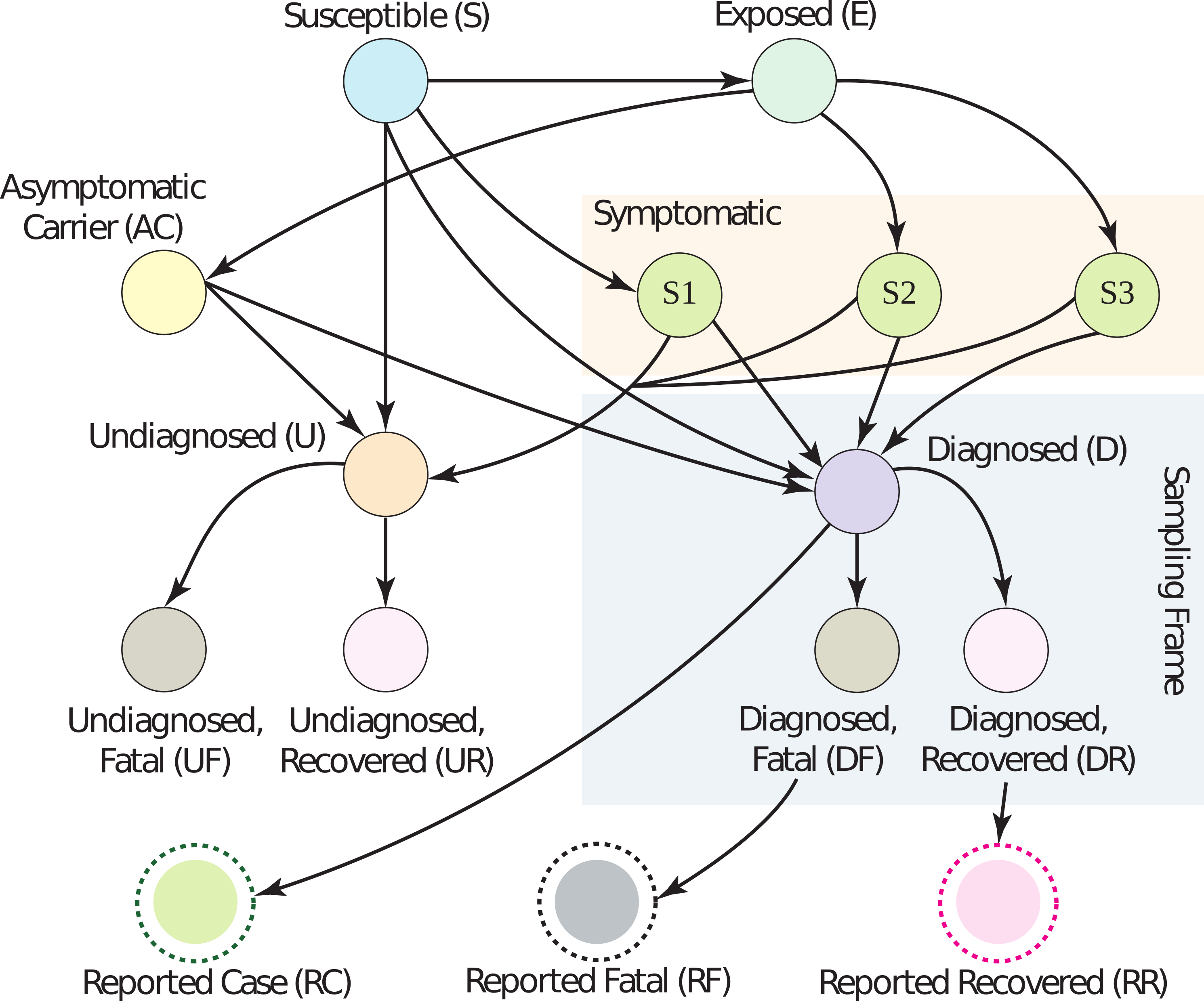
Dozens of biases can corrupt the estimation of the CFR. Surveillance data
gives partial information within the ‘sampling frame’ (light blue rectangle). Edges on
the graph correspond roughly to conditional probabilities; e.g., the edge from D to DF
is the probability a person dies if they are diagnosed with COVID-19.
In short, all CFR estimates are biased because the publicly available data is biased.
We have reasson to believe that we are losing at least 99.8% of our sample efficiency due to this bias.
There is a “butterfly effect” caused by non-random sampling: a tiny correlation between the
sampling method and the quantity of interest can have huge, destructive effects on an
estimator. Even assuming a tiny 0.005 correlation between the population we test and the
population infected, testing 10,000 people for SARS-CoV-2 is equivalent to testing 20
individuals randomly. For estimating the fatality rate, the situation is even worse,
since we have ample evidence that severe cases are preferentially diagnosed and
reported. In the words of Xiao-Li Meng, “compensating for [data] quality with quantity is
a doomed game.” In our HDSR article, we show that in order for the naive estimator $E_{rm naive}$ to converge
to the correct CFR, there must be no correlation between fatality and being tested — but
severe cases are much more likely to be tested. Government and health organizations have been
explicitly reserving tests for severe cases due to shortages, and severe cases are likely to go
to the hospital and get tested, while asymptomatic ones are not.
The primary source of COVID-19 data is population surveillance: county-level aggregate
statistics reported by medical providers who diagnose patients on-site. Usually, somebody
feels sick and goes to a hospital, where they get tested and diagnosed. The hospital reports the
number of cases, deaths, and sometimes recoveries to local authorities, who release the data
on a weekly basis. In reality, there are many differences
in data collection between nations, local governments, and even hospitals.
Dozens of biases are induced by this method of surveillance, falling coarsely into five categories:
under-ascertainment of mild cases, time lags, interventions, group characteristics (e.g.
age, sex, race), and imperfect reporting and attribution. An extensive (but not exhaustive) discussion
of the magnitude and direction of these biases is in Section 2 of our article. Without mincing words, current data
is extremely low quality. The vast majority of people who get COVID-19 go undiagnosed, there are
misattributions of symptoms and deaths, data reported by governments is often (and perhaps purposefully)
incorrect, cases are defined inconsistently across countries, and there are many time-lags. (For example,
cases are counted as ‘diagnosed’ before they are ‘fatal’, leading to a downward bias in the CFR if the
number of cases is growing over time.) Figure 1 has a graphical model describing these many relationships;
look to the paper for a detailed explanation of what biases occur across each edge.
Correcting for biases is sometimes possible using outside data sources, but can result in a worse
estimator overall due to partial bias cancellation. This is easier to see through example than it is to explain.
Assume the true CFR is some value $p$ in the range 0 to 1 (i.e., deaths/infections is equal to $p$). Then,
assume that because of under-ascertainment of mild cases, there are too many fatal cases being reported, which
means $E_{rm naive}$ converges to $bp > p$ (in other words, it is higher than it should be by a factor of $b$).
Also assume the time-lag between diagnosis and death causes the proportion of
deaths to diagnoses to decrease by the same factor $b$. Then, $E_{rm naive}$ converges to $b(p/b)=p$,
the correct value. So, even though it might seem to be an objectively good idea to correct for time-lag between
diagnosis and death, it would actually result in a worse estimator in this case, since time-lag is helping us out
by cancelling out under-ascertainment.
The mathematical form of the naive estimator $E_{rm naive}$ allows us to see easily what we need to do to make it unbiased.
With $p$ being the true CFR, $q$ being the reporting rate, and $r$ being the covariance between death and diagnosis,
the mean of $E_{rm naive}$ is:
This equation is pretty easy to understand. We wanted $mu$ to be equal to $p$. Instead, we got an expression
that depends on $r$, $q$, and $N$. The $r/q$ term is the price we pay if people who are diagnosed are more likely
to eventually die. We want $r/q=0$, but in practice, $r/q$ is probably much larger than $p$. (Actually, if we
assume the CFR is around 0.5% and the measured CFR is 5.2% on June 22, 2020, then $r/q ge 0.047 gg 0.005$.) In
other words, $r/q$ is the bias, and it can be large. The term $p$ is the true CFR, which we want.
And the factor $(1−(1−q)^N)$ is what we pay because of non-response; however, it’s not a big deal, because
it disappears quite fast as the number of samples $N$ grows. So really, our primary concern should be
achieving $r=0$, because — and I cannot stress this enough — $r/q$ does not decrease with more samples;
it only decreases with higher quality samples.
What are strategies for fixing the bias?
In our article, we outline a testing procedure that helps fix some of the above dataset biases. If we
collect data properly, even the naive estimator $E_{rm naive}$ has good performance.
In particular, data should be collected via a procedure like the following:
-
Diagnose person $P$ with COVID-19 by any means, like at a hospital.
-
Reach out to contacts of $P$. If a contact has no symptoms, ask them to commit to getting a COVID-19 test.
-
Test committed contacts after the virus has incubated.
-
Keep data with maximum granularity while respecting ethics/law.
-
Follow up after a few weeks to ascertain the severity of symptoms.
-
For committed contacts who didn’t get tested, call and note if they are asymptomatic.
This protocol is meant to decrease the covariance between fatality and diagnosis. If patients commit to
testing before they develop symptoms, this covariance simply cannot exist.
However, there may still be issues with people dropping out of the study; if this is a problem in practice,
it can be mitigated by a combination of incentives (payments) and consistent follow-ups.
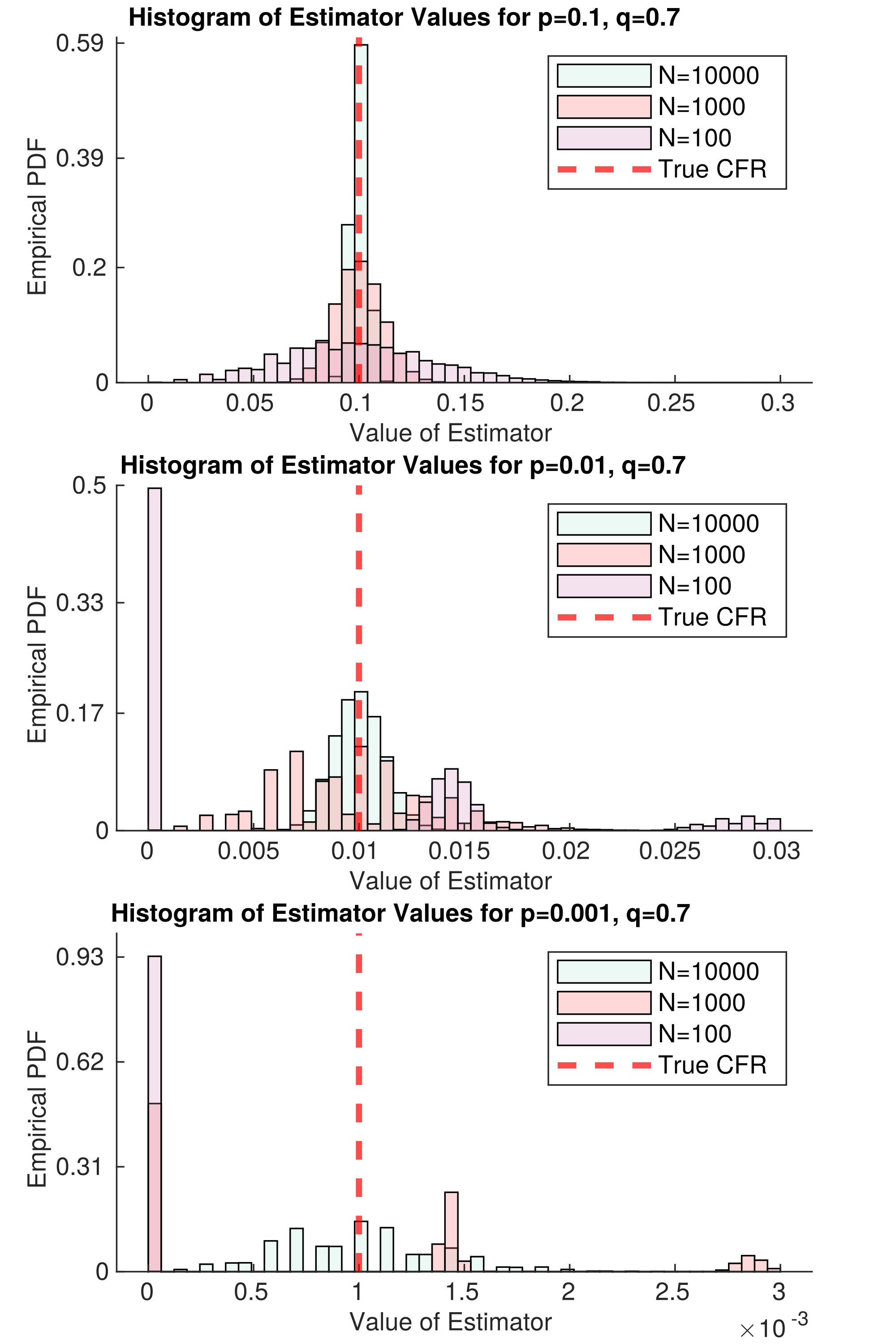
it requires more samples to estimate. The variable p is the true CFR, and q is the response rate. Each histogram represents
the probability the naive estimator will take on a certain value, given N samples of data (different colors correspond to different
values of N). The three stacked plots correspond to different values of p; the smaller p is, the harder it is to estimate,
since death becomes an extremely rare event.
Figure 2 represents an idealized version of this study. In the best case scenario, there is no
covariance between death and diagnosis. Then, we only need $N=66$ samples for our
estimator of the CFR to be approximately unbiased, even if $p=0.001$ ($1/1000$ cases die). Problems
remain in the case that $p$ is small; namely, death is so rare that we need tons of samples to
decrease the variance of our estimator. This will require lots of samples. But even if no deaths
are observed, we get a lot of information about $p$; for example, if $N=1000$ and we
have not observed a single death, then we can confidently say that $p<0.01$ within the
population we are sampling. This is simply because in the second panel of Figure 2,
there is nearly zero mass in the $N=1000$ histogram at $E_{rm naive} = 0$. With this in mind, we could
find the largest possible p that is consistent with our data — this would be a conservative upper
bound on $p$, but it would be much closer to the true value than we can get with current data.
This strategy mostly resolves what we believe is the largest set of biases in CFR estimation —
under-ascertainment of mild cases and time-lags. However, there will still be lots of room for
improvement, like understanding the dependency of CFR on age, sex, and race. (In other words,
the CFR is a random quantity itself, depending on the population being sampled.) Distinctions
between CFRs of these strata may be quite small, requiring a lot of high-quality data to
analyze. If $p$ is extremely low, like 0.001,
this may require collecting $N=100,000$ or $N=1,000,000$ samples per group. Perhaps
there are ways to lower that number by pooling samples. Even though making
correct inferences will require careful thought (as always), this data collection strategy
will make it much simpler.
I’d like to re-emphasize a point here: collecting data as above will make the naive estimator $E_{rm naive}$
unbiased for the sampled population. But the sampled population may not be the population
we care about. However, there is a set of statistical techniques collectively called
‘post-stratification’ that can help deal with this problem effectively — see Mr. P.
If you read our academic article, we provide some thoughts on how to use time-series data
and outside information to correct time-lags and relative reporting rates. Our work was very
heavily based on one of Nick Reich’s papers. However, as I claimed earlier, even fancy
estimators cannot overcome fundamental problems with data collection. I’ll defer discussion of
that estimator, and the results we got from it, to the article. I’d love to hear
your thoughts on it.
CFR estimation is clearly a difficult problem — but with proper data collection and
estimation guided by data scientists, I still believe that we can get a useful CFR estimate.
This will help guide public policy decisions about this urgent and ongoing pandemic.
This blog post is based on the following paper:
- On Identifying and Mitigating Bias in the Estimation of the COVID-19 Case Fatality Rate.
Anastasios Angelopoulos, Reese Pathak, Rohit Varma, Michael I. Jordan
Harvard Data Science Review Special Issue 1 — COVID-19: Unprecedented Challenges and Chances. 2020.