Large Language Models (LLMs) have revolutionized how we write and consume documents. In the past year or so, we have started to see them a lot more than just rephrasing docs: LLMs can now think before they act, they can plan, they can call tools like a browser, they can write code and check that it works, and a lot more – indeed, the list is growing quickly!
What do all these skills have in common? The answer is that they are all developed in what we call the post-training phase of LLM training. Despite post-training unlocking capabilities that would have looked magical to us a few years ago, it surprisingly gets little coverage compared to the basics of Transformer architectures and pre-training.
This tutorial was originally written for the Meta infrastructure team with the target audience of an infra engineer without expertise in LLM modeling who wanted to learn more about post-training to be able to contribute. I believe that this encompasses a large group of engineers: with Reinforcement Learning becoming mainstream, we need new infrastructure to be able to be productive, so bridging this gap is critical! I now share this broadly with the hope that many more folks across PyTorch Foundation will share a similar background and interest, and that they will also find this helpful, like our team did.
Primer on post-training
Post-training (sometimes referred to as “alignment”) is a key component of modern LLMs, and the way to “teach” models how to answer in a way that humans like, and how to reason.
Why is post-training different from pre-training, you ask? Post-training primes the model to have a conversation with a user, which follows a set of basic rules such as:
- In a conversation, there’s more than one speaker, and they all take turns talking
- You should listen before you talk to say something relevant
We find these obvious, but pre-training is only doing next-word prediction to teach the model about the world, so your data there is completely unstructured, so the model never learned these basic rules. Indeed, a model coming out of pre-training is often bad at understanding that it should stop talking after a while and will blabber on forever, kind of like a Google autocomplete box.
Furthermore, it’s also useful to impose some ground rules to the model that take absolute precedence over everything else. This is done in post-training through a system-prompt (and/or through Supervised Fine Tuning (SFT)/reward shaping, see later).
Post-training data format
Chatting with these models is possible via some plumbing that happens behind the scenes. Every time you talk in a chat window to a service like ChatGPT, you’ll see a UI like this:

What actually happens is that the post-training structure is plumbed for you, and the model will see something like this (using the data format for Llama 3):
<|begin_of_text|>
<|start_header_id|>system<|end_header_id|>
… <|eot_id|>

<|start_header_id|>user<|end_header_id|>
What is the capital of France?<|eot_id|>

<|start_header_id|>assistant<|end_header_id|>
The capital of France is Paris

<|start_header_id|>user<|end_header_id|>
How many people live there? Tell me just the number<|eot_id|>

<|start_header_id|>assistant<|end_header_id|>
START FILLING FROM HERE
Note that the basic interface of the LLM is unchanged: you provide some text, and it will continue it to infinity and beyond.
What this clever plumbing does is to make sure that the model receives all the metadata to know that the previous speakers have spoken (and it should not impersonate them!!), and to stop once assistant is done talking. Again, the model will happily continue filling, but after we see a <eot_id> token (“end of turn”), we stop the model from continuing and we send it back to the user.
Note that the model won’t do any of this: for all the cleverness we perceive, they do remain just text fillers that require this hand-holding.
This format is a bit hard to read, but you can essentially conceptualize this as something like:
<system> You are a helpful assistant bla bla </system>
<user> What's the weather in Paris? </user>
<assistant> ANSWER HERE
Fun fact: the model will happily play either part! You can totally play the assistant and let it play the user by feeding it the right text structure – the model simply takes over and completes text no matter what you provide. Try it out using a local model or an API (products like ChatGPT will do this plumbing for you and you can’t override them). Obviously, a model is very sensitive to its own format so make sure you use the correct one.
Post-training techniques
Post-training is a rapidly-changing field where different teams will use different techniques.
Let’s look at this pipeline as described by the OLMo 2 paper:
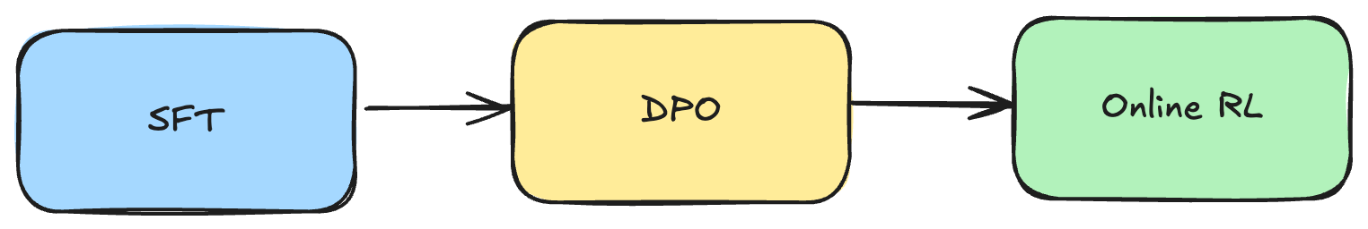
The following section goes through each box one by one.
SFT: Supervised Fine Tuning
The focus in SFT is imitation. It’s simple conceptually: you teach the model to forcefully learn an answer step by step.
If this was chess, you could SFT by training on Magnus Carlsen’s games, where you would forcefully teach the model that it should follow the moves that Magnus took at each and every step. You can see the limit of SFT: you can reach Magnus’s ability, but he is going to be your ceiling as you have no way of trying to uplevel him (as opposed to Reinforcement Learning (RL) where you can keep trying until you get really good, see later).
In the case of LLMs, you learn the ideal answer word by word, so your loss function is simply cross-entropy against the output layer with the ideal “class” being the id of the “correct” word). A common question we get is: isn’t this the same as pre-training, then? It is indeed very similar, with only one crucial difference: you only condition on the prompt; you don’t learn the prompt. Why? Because what you want is to learn how to answer that question, not learn the question itself.
Remember: unlike pretraining, in post-training we have this structure with system prompt, and user prompt (see Post-Training data format right above). These are the parts of the input that we want to condition on, but not learn from. We do it by feeding the whole sequence through (including system prompt and user prompts as well as any special characters) without any masking, but when we compute the loss, we mask the loss of every token that is not the actual response. We don’t mask the prompt in input as we do want its contribution into conditioning the input. We mask it in the backward step to prevent it from contributing to the loss).
They are so similar that in practice, SFT can piggyback on all the infra that was already built for pretraining: indeed, training platforms like Megatron use the same dataloader and trainer class as the pretraining step, and simply set an argument to mask the loss over the prompt.
That said, the scale for these is nowhere near pre-training – you should expect to do SFT within a few million samples at the maximum, so only a few B tokens, whereas pre-training will crunch trillions of tokens.
Who writes the response?
SFT learns word by word, which limits it in two important ways:
- Your ceiling is represented by whoever wrote your answer (see previous paragraph)
- Critically, you are strongly dependent on data quality. In practice, your ceiling ends up being determined by your worst answers rather than your best. When you source answers from people, you cannot expect all of them to be of the same, amazing quality. Some of them will not be great, and they have a ton of impact on the quality of your model.
So, what do we do? We can’t fight human nature, so the idea is to instead have the LLM generate the responses it will train itself on. This seemsunintuitive at first, but the idea is called Rejection Sampling (see the Llama 2 paper for more info). It works because we don’t just generate one answer (then yeah, it would not improve itself) but we generate many (usually 10), from multiple different checkpoints, random seeds, system prompts, etc, to elicit diversity. Then, we keep the best answer (as ranked by a pipeline, often including other models such as the human preference reward model) and we add that to the bank. If you have a background in Machine Learning (ML), you can think of this approach as a way to kinda, sorta, distill from a kinda, sorta, ensemble into a single model (very handwavy, I know!).
You can ride this loop through many iterations. If done right, you can climb the hill and get better and better.
A primer on Reinforcement Learning
RL is a wide spectrum that includes the famous Reinforcement Learning from Human Feedback (RLHF), but it’s not limited to it.
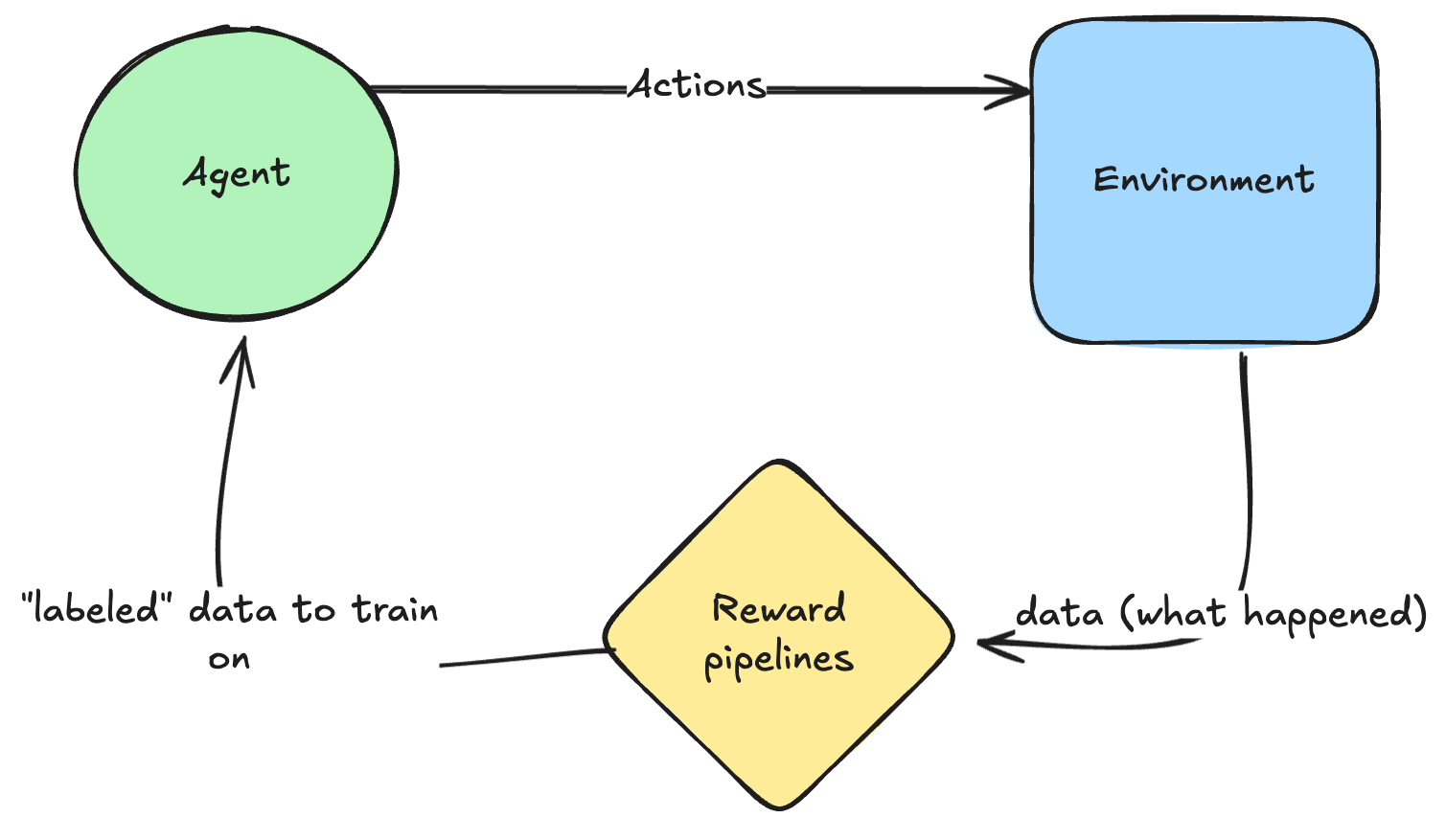
In general, the whole idea behind RL is that you are now an agent that can take actions against an environment and get to observe what happens and obtain rewards from it. You can think of these rewards as generating a “label” that you can then train on – though backprop is gonna look different (more on this later).
How do you train?
Backpropagation does happen in RL, but with key differences from the neat forward-backward loops we enjoy in supervised learning.
The key difference is that in RL we unfortunately do not have a differentiable cost function, like Cross Entropy or Mean Square Error (MSE). Rewards (and tools like browsers) are not differentiable, so you can’t just backprop through them – which is very unfortunate.
So what we do instead is a very crude approximation: we simply operate on the logprobs in output of the model and make them bigger if the action was good, and make them smaller if it wasn’t – then, we backprop into the model to tweak all previous layers to make this happen. Note that this is far less efficient than optimizing a supervised cost function like MSE and Cross Entropy: supervised cost functions return a dense vector of gradients, whereas here we only get a single scalar back from a whole episode, which is far less efficient as we get less “learning juice” per interaction.
There are more bells and whistles around the RL learning process, with different algorithms making different choices on how to answer the major problems (vanishing/exploding gradients, sample efficiency, infra optimization and so on,) but this is the general gist. The Appendix gives you a detailed step-by-step derivation of Proximal Policy Optimization (PPO).
Let’s look at this from an infra perspective: compared to “standard” supervised learning, you need to run a ton of inference on the model, which is more expensive (autoregressive, token-by-token vs feeding a whole existing sequence through in a single forward pass), requires more infra (KV cache etc), is harder to batch, and so on.
Despite the training objective being so crude, it actually works very well in the presence of sparse or long-term rewards, while SFT requires rewards to be dense (you are told what each token should be).
Following the chess analogy:
- SFT teaches the model to copy move by move
- In RL, the model is rewarded when it wins the match (which can be after 20 moves). The training algorithm will favor model configurations that lead to more reward, more often (given some exploration/exploitation trade-off).
While you start off much weaker, eventually, by playing enough games, you can reach Magnus’s level, and far surpass it – in other words, the ceiling you can reach is much, much higher.
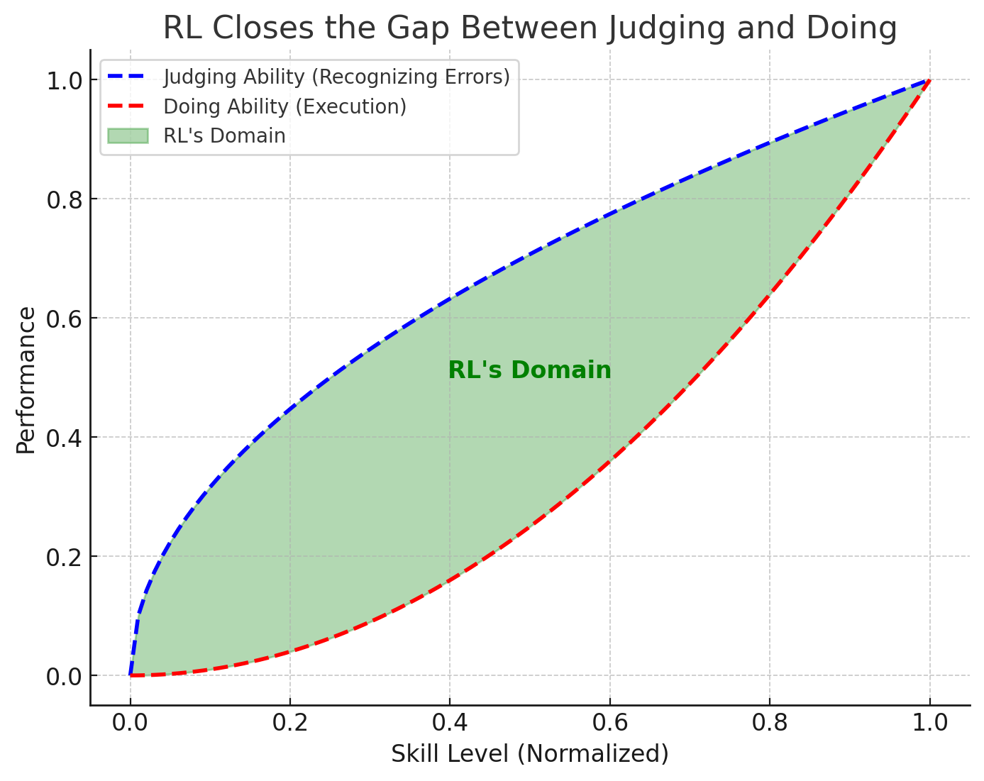
In a way, you can view RL as a magical machine that closes the gap between judging and doing: that is a very big gap! I can recognize when a F1 driver messes up, but I can’t do what even the worst F1 driver can do. RL can transform any armchair driver into an actual driver 
If you want a one-liner, “if you can judge it, you can learn it!”.
Reward hacking
Note one thing: your ceiling is still going to be represented by your ability to judge (blue curve), which is determined by how good your rewards are: for something like games, rewards are super clean (you know when you win with 100% precision and recall), so the sky is the limit. You can apply RL to anything though, but if you can’t judge very well, your agent is going to learn noise.
A corollary to RL being limited to your judging ability is that it may learn behaviors that you didn’t intend: RL will do anything in its power to maximize the reward you give it, so the model will do exactly what you asked, not what you wanted. We call this reward hacking, even though the model isn’t responsible for this, we are when designing the incentives!
One example to drive this home: RL found out that Super Mario 1 has always had a bug for over 30 years where after you jump, if you turn around you are invulnerable for a single frame. Given that its reward is to maximize the score and that if you clear a level faster, your score will go up, it exploits the hell out of this bug to get a higher score (and thus a higher reward).
What developers wanted:
- Maximize score
- Still play like a human
- Don’t exploit bugs
What developers asked:
- Maximize score
Note: this happens with humans too! We just call these Perverse Incentives, but they are literally the same thing. The British government, concerned about the number of venomous cobras in Delhi, offered a bounty for every dead cobra. Initially, this was a successful strategy; large numbers of snakes were killed for the reward. Eventually, however, people began to breed cobras for income.
Applications to LLMs
Similar to the chess example, RL can have a higher ceiling than SFT and thus it’s the method of choice to teach the model how to converse with humans in a way we like (RLHF), how to reason, and so on.
As we have just seen, the ceiling you can reach is set by how good your rewards are: if you use a classifier to provide a reward, your ceiling will be the accuracy of that classifier.
RLHF
One such classifier is human preference. It’s hard to write a rule for how to write with a style that humans like, so what we do instead is train a classifier to score these. We monitor its performance via accuracy and PR AUC (this one is only necessary if you want a continuous score to rank on; otherwise, point estimates like F1 or Accuracy are all you need). Once you have this classifier, all you need to do is run RL against it and optimize against its feedback.
DPO: Direct Preference Optimization
Now let’s look at the second box in our LLM post-training pipeline. DPO is an algorithm that is used specifically for RLHF of LLMs, it is not a general RL algorithm (unlike PPO and friends, which can be used to train robots and anything else you want).
In fact, technically, DPO is not even a proper RL algorithm; it just pretends to be one! The whole idea of DPO is that if you make some reasonable assumptions, you get to have a differentiable loss function while still training for RLHF.
To be more accurate, DPO allows us to have a supervised learning solution to a Markov Decision Process under certain assumptions (see later), which is a big deal as normally the only general way to solve MDPs is via Reinforcement Learning (and its inefficient cost function).
The core idea behind DPO is this: instead of having a separate reward model, you can recycle your LLM to be both your policy model and your reward model. Why? Because your LLM gives you the probability of an answer given a question. So, if you have a preference pair you can simply say that for the same question, you want the probability of the preferred answer to be high and the probability of the rejected answer to be low. In other terms, you want to maximize which leads to a very nice differentiable function!
DPO is dirt cheap to run compared to PPO and other RL algorithms that instead need to sample multiple answers by running a ton of inference. The negative is that DPO doesn’t explore, so there’s also a limit to how good you can be. Here’s a more detailed comparison to a “real” RL algo like PPO (which we are going to see in more detail next).
| Feature | DPO (Direct Preference Optimization) | PPO (Proximal Policy Optimization) |
|---|---|---|
| Optimization | Supervised Learning | Reinforcement Learning (RL) |
| Data Needed | Fixed dataset of (prompt, preferred, rejected) pairs | Rollouts + Reward Model |
| Loss Function | Binary classification-like loss | Clipped policy gradient loss |
| Exploration |  No (fixed dataset, no exploration – fully Offline) No (fixed dataset, no exploration – fully Offline) |
 Yes (policy can explore new responses – Online algo) Yes (policy can explore new responses – Online algo) |
| On-Policy? | Off-Policy (learns from fixed data) |
On-Policy (requires new rollouts) |
| Compute Cost | Low (single forward pass per pair) |
High (rollouts + PPO training) |
| Training Stability | Stable (like fine-tuning) |
Unstable (RL variance) |
| Convergence Speed | Fast |
Slower (needs many rollouts) |
| Performance limited by | Data |
Compute (better place to be) |
| Best for | Cheap alignment using human preferences | More flexible but expensive fine-tuning |
Online RL
The third and final box in our sample LLM post-training pipeline is Online RL. The “standard” algorithm is PPO (Proximal Policy Gradients), which was made by OpenAI in 2017. Another algorithm that’s widely adopted is GRPO (Group Relative Policy Optimization, introduced by DeepSeek).
Key concept: On-policy vs Off-policy
A policy is simply the LLM you are training. Being on-policy means that every interaction with the environment is coming directly from the model being trained. This makes the most sense as that is how we learn with a private tutor: we try something, we make some mistakes, we immediately get feedback, and try again having this knowledge. This is much better than learning off-policy where you are shown what someone else did in this situation and you can learn from it – that someone else can (and often is) be a past version of you, so it’s common to keep around a memory of what you did in the past in a replay buffer for later use.
RL algos belong to one of these two families, with PPO belonging to the on-policy side and Q-learning (like DQN) being in the off-policy camp.
| Feature | On-Policy RL (e.g., PPO) | Off-Policy RL (e.g., DQN, DPO) |
|---|---|---|
| Definition | Learns from data collected by the current policy | Learns from previously collected data (even if from old policies) |
| Exploration | Yes (continuously generates new rollouts, explore-exploit tradeoff baked into the logits of the policy network already – naturally starts by exploring a lot, and gradually moves towards exploiting) |
When run offline, you never explore as you just recycle old data you generated before (like DPO).
You can run it online and explore, but the exploration strategy is left to you to define (eg epsilon-greedy) |
| Infra Efficiency | Low (needs to always generate data online) |
Higher (reuses past generations) |
| Training Stability | Unstable (policy keeps changing) |
More stable (fixed dataset or replay buffer) |
| Compute Cost | High (requires frequent rollouts)
The cost is mostly due to the sync nature of the training loop (collect → train → collect → train) |
Low (trains on stored data) |
| Example Algorithms | PPO, A2C, TRPO | DQN, DDPG, SAC, DPO |
| Best for | Situations where continuous exploration is needed | When you can store and reuse past experiences |
From an infra point of view: Online vs Offline RL
On-policy vs Off-policy is looking at things from the perspective of the model training dynamics. If we look at things from an infra perspective, we should think about Offline (using static data that we simply reload while we train) vs Online (we generate data live). These two concepts map well to Off-Policy and On-Policy, so are sometimes used interchangeably, though technically they are still a bit different:
- If you are learning offline, you can only learn off-policy (as the data was generated by another model and saved). Rejection Sampling and DPO are off-policy, offline algorithms. This is the simplest thing for infra.
- If you are learning online, being on-policy or off-policy is actually more of a spectrum once you start thinking about using multiple machines and synchronizing. If you want to be strictly on-policy, it means you are training with batch size = 1, then sampling from that model, and introducing barriers throughout so that the model is updated constantly and no new trajectories are sampled before we re-scatter all the weights to all nodes.
In code:
# Idealized PPO training loop

collector = CollectorClass(model)

for i in range(num_collection):
    collector.sync_weights_() # align weights across all workers
    # resume collection and put trainer node on hold <- this is bad!
    data = next(collector) # collect data
    # Put collector nodes on hold <- this is bad!
    for j in range(num_epochs):
        for batch in split_data_randomly(data):
            loss_val = loss_fn(data)
            loss_val.backward()
            optim.step()
            optim.zero_grad()
Therefore, some degree of “off-policiness” is desirable and acceptable. This goes with many questions: to which extent is it the case? How frequently should you update the collection weights? How can you overlap the weight sync, the collection process, and the model training to maximize the throughput?
I don’t want you to leave this section with the idea that off-policy and offline algorithms are necessarily the pits and to be avoided in all cases. In fact, the first two pieces of our pipeline in Llama (SFT and DPO) are essentially a way of solving the alignment Markov Decision Process via a supervised cost function. These are acting as “kind of” offline, off-policy RL:
- Our SFT data is coming from Rejection Sampling, meaning that we generate it with the model itself. While we don’t use a proper off-policy RL algo like DQN, rejection sampling done this way is a form of offline policy optimization.
- Similarly, we have seen that DPO is also a form of offline policy optimization that also gets away with doing actual RL gradient updates, which are slow and unstable.
Different groups found different recipes in how to leverage all these techniques and how to combine them, but not every group publishes this information.
Beyond RLHF: a general paradigm
There is nothing limiting us to sticking to human feedback – and indeed, we are not. If you want to learn how to code well, you can instead provide a testing harness and give a reward that’s proportional to how many tests you pass. If you want to learn to solve integrals, you can use Wolfram to check if your equation is correct.
In short, you can build reward pipelines by mixing Software 1.0 and Software 2.0. The common patterns are:
1. Reward Models. A classifier that gives a continuous score from 0 to 1 (or sometimes even unbounded). Useful for ranking many answers (just sort on it), especially in domains where you can’t easily express what you want (human preference, writing style, etc).
a. Outcome Reward Models. ORMs provide feedback based on the final result and the final result only of a chain of thought. These are the most common ones – indeed, if someone just says “Reward model”, it’s one of these.
b. Process Reward Models. In the example above (chess), the reward is sparse: it only occurs when the game is won or not. Intuitively, having dense rewards could help the agent to get a more fine-grained knowledge of what behaviour is or is not desirable. This is what PRMs do: they don’t just judge the final output, but the whole sequence of steps. For example, a PRM would judge an entire chain of reasoning thought and make sure that every step is sound. These are not commonly used (at least not yet) as they tend to be very noisy.
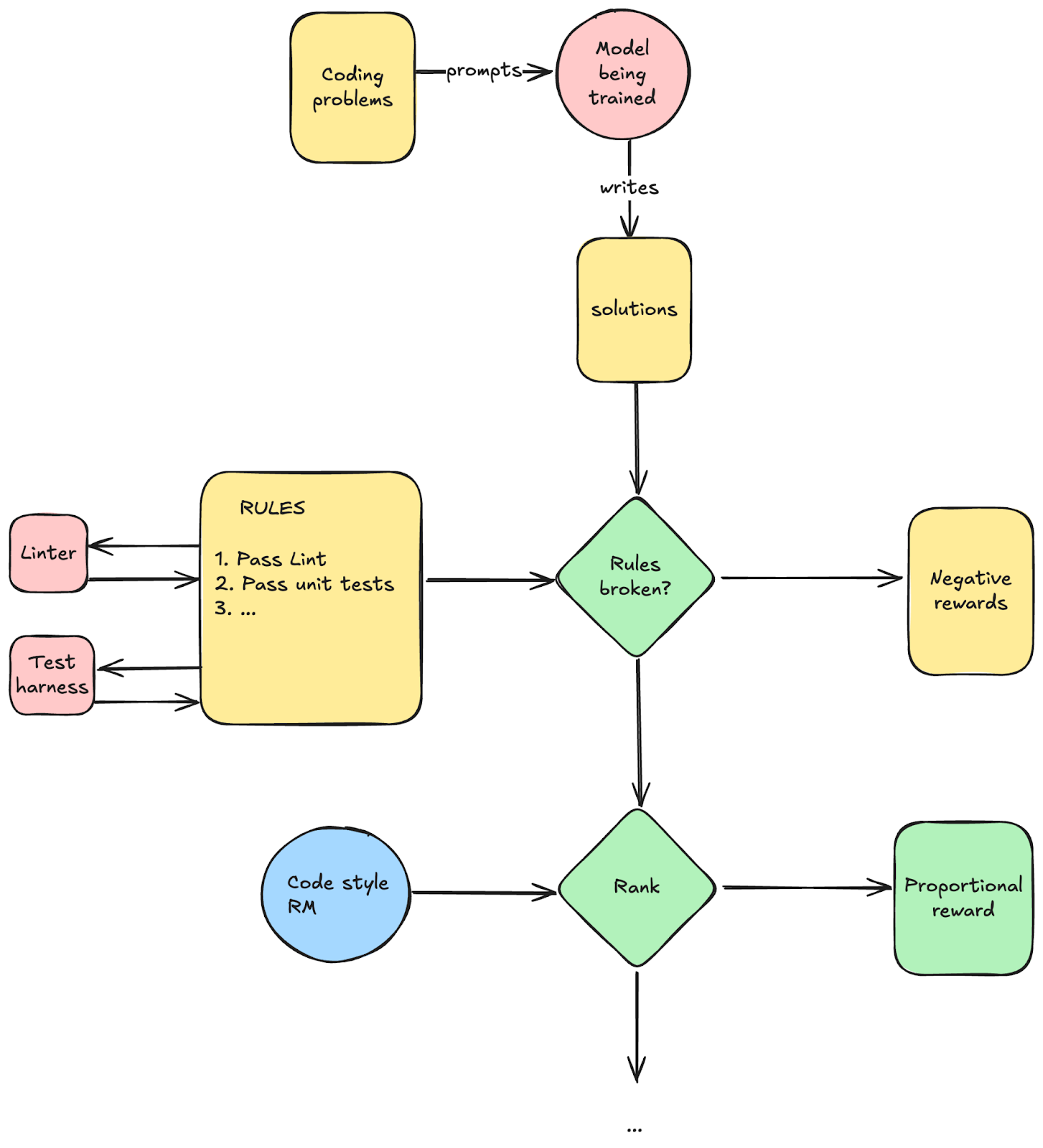
2. Rule-based rewards. You can write down a list of rules and put rewards associated with each (or respecting them as a whole).
a. Software pipelines. These run “normal” software 1.0 and give you a reward based on that. For example, passing test cases for coding or passing linting.
b. Judges. When you can’t check if rules were followed via a traditional software pipeline, you can instead use an LLM to verify if rules were respected for you. For example, you can write a set of safety rules that shall not be broken, eg: “No mentions of sexual stuff”, and a judge can ask the question “Were all the rules followed?”. NOTE: this is different from a continuous-score reward model, because you only get a binary answer (rules followed or not). You can’t rank many answers on this, so this is instead used to provide a negative reward if some rules were broken. In practice, you often don’t even train these and instead simply prompt a foundation model to judge for you.
These are components of what can become very sophisticated reward shaping pipelines. For example, you can imagine having a complex Directed Acyclic Graph (DAG) of these to give very granular rewards.
Simple example for coding:
This has infra implications:
- Sandboxing for the test harness and any other binaries you need to run
- Where do we host all these reward models? You can have many, and they can be big (don’t think of these as small dedicated classifiers! They are often just as big as the model you are training!).
- We should expect more and more engineers to develop better and better reward pipelines (more granular, to shape the model’s behavior). This can become the place where engineers push their contributions. These pipelines themselves can be a useful thing to have a Hub around and to crowdsource development.
Test-time compute and reasoning
Test-time reasoning is a major trend that came out in the last year from OpenAI, famously replicated by DeepSeek in their DeepSeek R1 paper.
Let’s dive deeper into what this is.
In short, this builds upon previous work (such as Chain of Thought and ReAct loops) that figured out that letting the model “talk aloud” with itself before committing to an answer can greatly improve the quality of its answers, particularly on certain domains like math. This ability came spontaneously, without ever training the LLM for it. So naturally, the next step was to figure out a way to train the LLM to get better at this “thinking step”.
We don’t know what technique OpenAI employed, but the most surprising finding of the DeepSeek R1 paper was that you don’t need a super clever setup to induce this learning. In fact, they show that simply providing the model the space to think (by simply instructing it to fill text between a <think>token and a </think> token, and for that text not to be empty.
This is the system prompt they used:
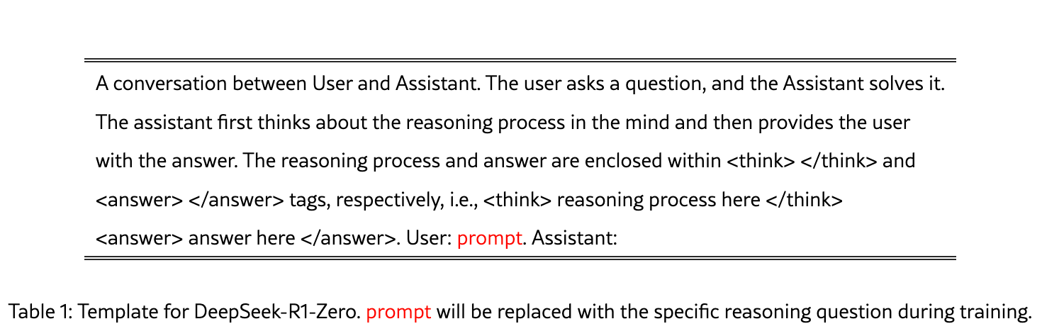
Once this was in place, they went into reward modeling.
Annotated excerpts from the paper
I strongly recommend reading the whole DeepSeek R1 paper, as it is very well written. Here, we quote a few sections of the paper with my own comments to provide context for a reader that’s not a specialist in this field.
Section 2.2.2: Reward modeling
The reward is the source of the training signal, which decides the optimization direction of RL. To train DeepSeek-R1-Zero, we adopt a rule-based reward system that mainly consists of two types of rewards:
|
Comment: This is all pretty standard stuff as we have seen. Conceptually, this is simple. Doing it in practice requires craft from the ML engineers to craft good rewards that aren’t noisy and that nudge the RL process in the direction you want.
|
Comment: Smart!!! A simple way of nudging the model to start leveraging the thinking process. Otherwise, it may not consistently explore adding thinking between these <think> and </think> tags. Adding a strong negative reward when it doesn’t do it straightens it out and constrains the exploration to using them. They stop here for R1-Zero, but you can actually keep going to more intricate reward modeling. For example, R1-Zero sometimes thinks in a mix of English and Chinese, so you could fix this by adding a prompt (and then a reward) for thinking in English. You can also add intermediate negative rewards if the thinking process is judged not “good” in some way (inconsistent, etc) to further nudge the model. You can see that this is a general paradigm…
|
Comment: Maybe someone in the community will eventually figure out how to make process RMs work…
Other observations
- The “Aha” moment:
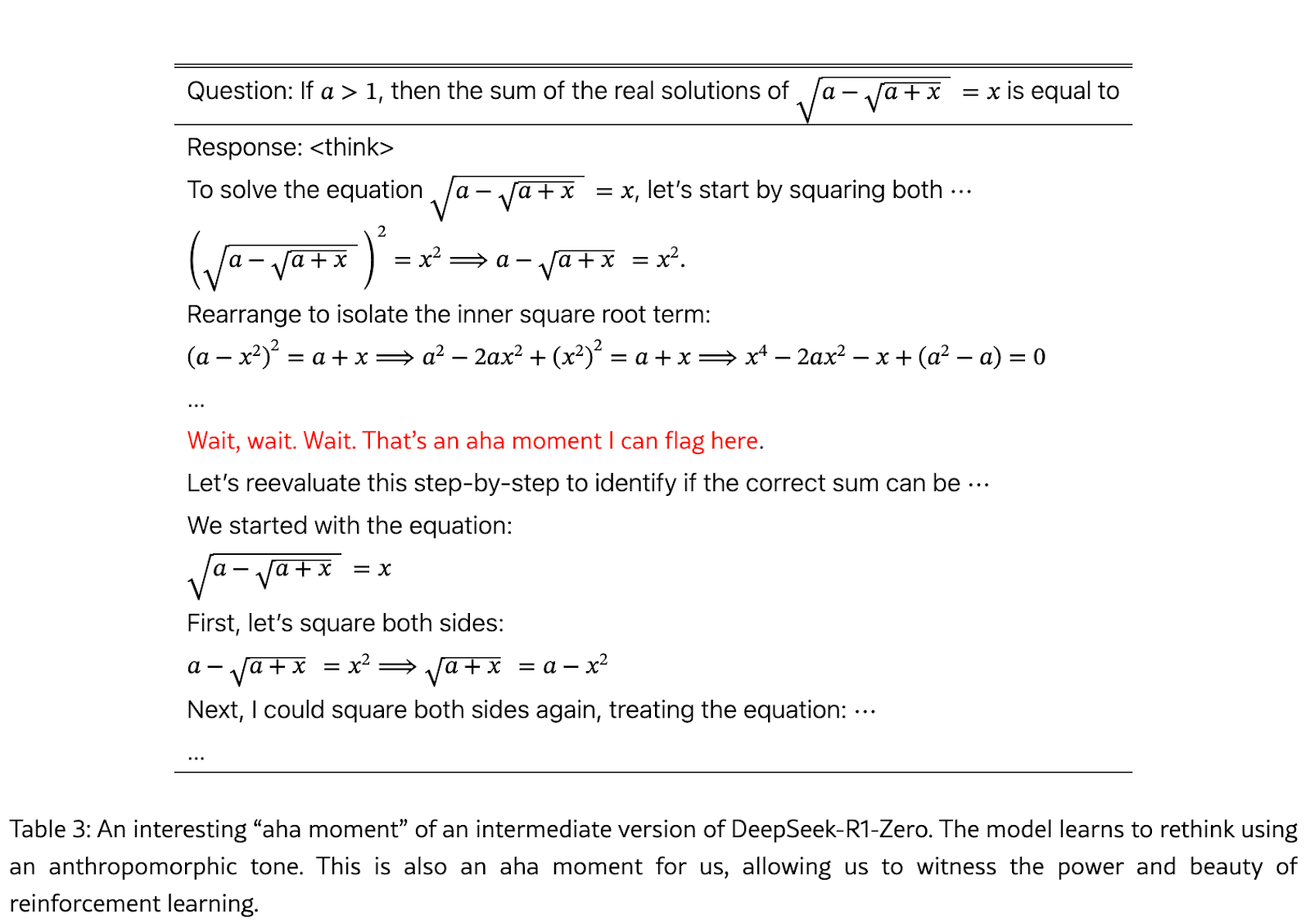
This one is very interesting to me as RL essentially learns to backtrack on its own. That’s pretty cool, and I honestly didn’t think that this would happen. I imagine that you can improve on this via search: beam search is the simplest, and you can go into tree search algos from there like MCTS. Now that we have a baseline that works, I think that we are going to see faster progress on all these more complex methods. This IMHO a strongly misunderstood part of this work: DeepSeek hasn’t shown that you don’t need all this compute in AI, quite the opposite! They have just shown that you don’t need complex methods to get started, and that simple methods with scale are sufficient – a lesson we keep learning in AI.
Increasing thinking time (and test-time compute) on its own:
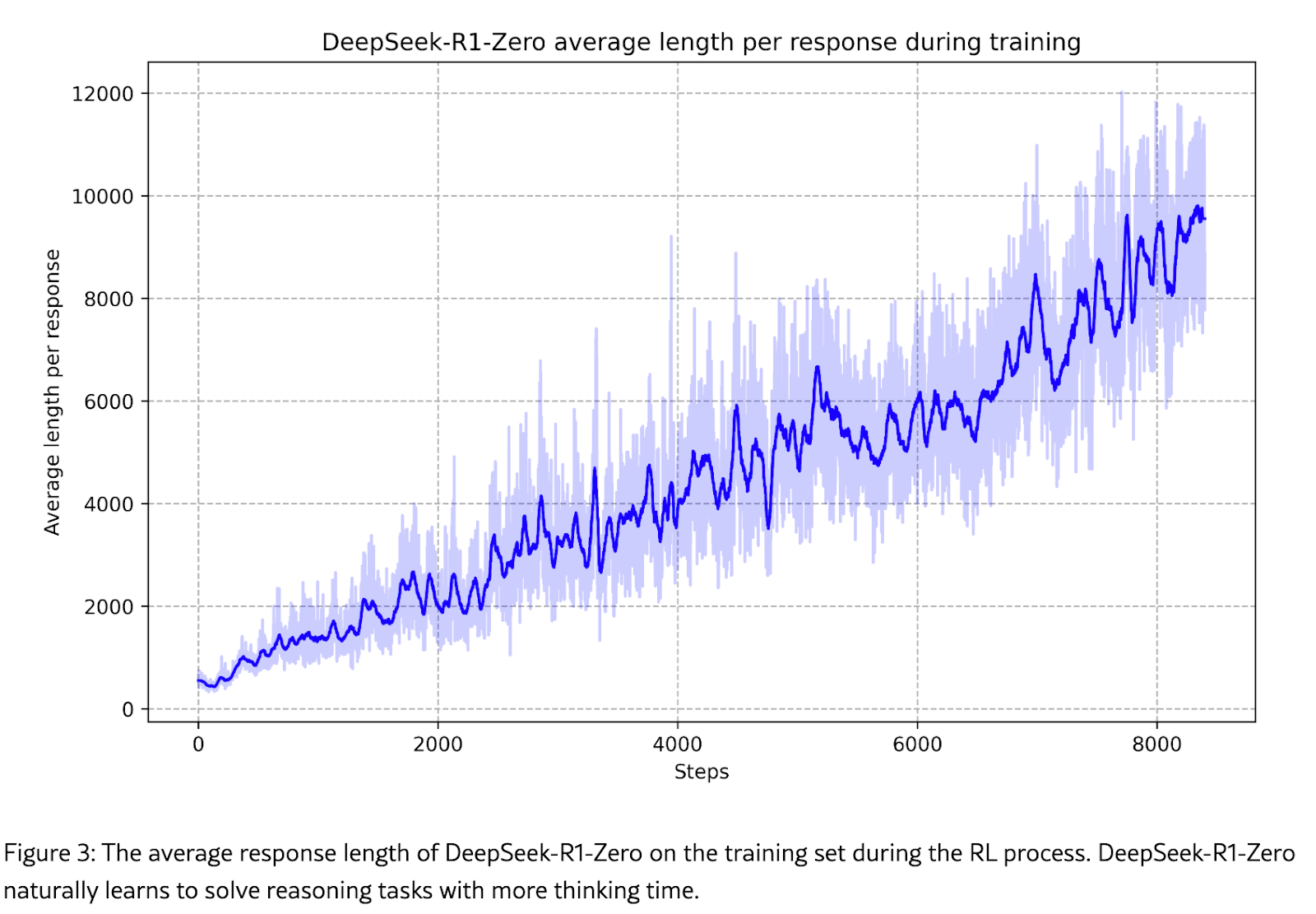
Since they never gave the model any penalty for thinking too long, RL figures out that there is simply no downside to thinking for longer and with each passing iteration, it just keeps going in the direction of longer thinking traces. This is expected. I would imagine that if they kept going, the model would also automatically learn to stop at its max sequence length, as then it wouldn’t be able to remember its whole reasoning trace, so going further wouldn’t help (and it may harm).
Once again, the model learns that test-time compute is good, and thus we should expect compute demands to go up.
Appendix A: Diving deeper into PPO
Let’s go deeper into backprop in RL.
Let’s start from the “basic training loop” in supervised ML (no RL):
loss_fn = nn.CrossEntropyLoss()
for batch in dataset:
        x, y = batch
        y_hat = model(x)  # One forward pass only
        loss = loss_fn(y, y_hat)
        loss.backward()  # One backward pass
Recall that in RL we do not have a nicely defined cost function, so instead we are just making an action more likely if it was good, and less likely if it was bad. How do we do that?
Our model already outputs a probability distribution over actions, so the final layer will have its Softmax over all the actions. What we want to do is to give a positive gradient to the good actions and a negative gradient to the bad actions.
So, basically, we wanna do something like this:
model.weights.grad[good_actions] += delta
model.weights.grad[bad_actions] -= delta
Autograd can do that for us: to get a constant delta added to the gradient, we need a function that, when differentiated, gives us this delta. The answer is multiplication. So, our “cost function” is simply log_probs * per_token_reward.
Let’s stay high level and develop this gradually (the PPO loss looks quite scary otherwise):
for batch in dataloader:  # Iterate over dataset (prompts)
    prompts = batch        # Get input prompts: (bsz, prompt_lens). Can be ragged, or packed.
    responses, log_probs = model.generate(prompts)  # Autoregressive
generation! MANY forward calls, need KV cache etc. If this is not clear to
you, read this appendix.

# Also note: we NEED to return log_probs for all the intermediate
generations and note that we are not detaching them from the graph as we
are gonna need them later.

   # responses and log_probs are of size (bsz, response_lens).
Also ragged/packed.

    sequence_rewards = get_feedback(responses)  # Get rewards (e.g., human
preference or heuristic).

    # Note that rewards CAN be negative, in that case this sign will be
negative.

    # This is a tensor of size (bsz,).

    per_token_reward = discount(sequence_rewards)  # This one is (bsz,
response_lens). A simple way to discount is to multiply tokens by a factor
gamma (eg 0.99).  So the last token gets reward of 1, the second-to-last
gets 1*gamma, then the previous gets 1*gamma*gamma and so on. You don't
want to maximize only your reward at time t but the sum of rewards till
the end of the episode

    optimizer.zero_grad()  # Reset gradients

    # Manually nudge log-probs based on reward signal

    adjusted_log_probs = log_probs * per_token_reward # this is a
stochastic estimator for the gradient of the reward expectation given your
stochastic policy - in other words: on average, the gradient of that thing
points to where the policy is doing good!

    loss = -adjusted_log_probs.sum()  # Equivalent to maximizing
probability of good actions

    loss.backward()  # Still ONE backward call! PyTorch knows what to do.

    optimizer.step()  # Update model parameters
Note that while we do multiple forwards (due to autoregressive generation), we only need one backward (well, assuming we keep the graph around. If you have these generations done by VLLM or something else, then we are gonna need one more forward pass here to materialize the graph on this side which shouldn’t be too bad…).
Now let’s make this more realistic
The above is all we are doing conceptually. Except that when you go and try it, everything will diverge 
Let’s make these changes:
- Adaptive delta. Using a static delta is suboptimal since the magnitude of the update should be proportional to how good a choice is. Instead of manually nudging logprobs, we can let backprop do the work for us. If you want to increase probabilities, you can simply maximize log-prob. To do it in gradient descent, we minimize the negative logprob. This is the Policy Gradient Loss function:
policy_gradient_loss = - (rewards * log_probs).sum(dim=-1).mean()

policy_gradient_loss.backward()
- Reducing variance. If we were to train with just the above, some responses would get huge rewards and others would get zero, leading to unstable training. A way to mitigate this is to introduce a baseline, which is the expected cumulative reward for an average move: not terrible, but not great either. The intuition behind this is that the goodness of a move always depends on the available alternatives: for example, getting 1M dollars seems great until you realize that you had the option to get 100M dollars.
This “goodness” of a move with respect to the baseline is called the advantage, a core concept in RL.
How do we predict the baseline score (also known as the value of a state)? Two ways:
- Value Network. Train a model to do that for you: you can train a value network to estimate what this baseline should be.
- Monte Carlo. Simply run a bunch of generations (often 4-5 is enough) and the average cumulative reward of all your generations is your estimate of the value.
Now our code will look like this:
for batch in dataloader:
    prompts = batch
    responses, log_probs = model.generate(prompts)

    rewards = discount(get_feedback(responses))  # Already discounted

    for n in range(epochs):
        for _prompts, _log_probs, _rewards in make_minibatches(
            prompts,
            log_probs,
            rewards,
            ):
            values = value_network(_prompts)  # Predict baseline V(s)
            optimizer.zero_grad()
            # REINFORCE with baseline
            advantages = _rewards - values  # Compute advantage estimate
            loss = - (advantages * _log_probs).sum(dim=-1).mean()
            loss += advantages.pow(2).mean()
            loss.backward()
            optimizer.step()
Believe it or not, that is still unstable! RL is just massively unstable and finicky (though it is surprisingly well-behaved for LLMs, compared to other fields). One reason is that the distribution of rewards can have a very long tail, i.e., your gradients do not behave very nicely. So, in practice we really really gotta make sure that updates are well-constrained so that training behaves nicely.
What PPO does is basically trying to enforce stability by cramming four different constraints:
1. Standardize advantages
The code above multiplies by the raw advantage which, despite our best efforts at baselining, can still lead to huge updates that will destabilize training. One way to make things well-behaved is to simply shift them to zero mean and scale them to unit variance.
advantages = (advantages - advantages.mean()) / (advantages.std() + 1e-8)
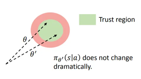
2. Importance Sampling
That is still not enough. To improve further, we are gonna enforce that updates stay constrained within a trust region. PPO does this by preventing updates that are too large relative to the old policy (so yes, it needs to keep around the model at time t-1):
So now we do this instead:
old_log_probs = get_old_log_probs(prompts, responses).detach()  # Log
probs from previous policy

importance_sampling_ratio = torch.exp(log_probs - old_log_probs)

safe_advantages = importance_sampling_ratio * advantages
3. Clipping large updates
Oldest trick in the book. If you risk having too big a gradient, simply clip it.
old_log_probs = get_old_log_probs(prompts, responses).detach()  # Log
probs from previous policy

importance_sampling_ratio = torch.exp(log_probs - old_log_probs)

clipped_sampling_ratio = torch.clamp(ratio, 1 - epsilon, 1 + epsilon)

even_safer_advantages = clipped_sampling_ratio * advantages
4. Taking a min()
This one was the most surprising to me. Instead of just using the clipped advantages, you actually want to run a minbetween the clipped and unclipped version. The reason is subtle: RL will try to maximize its rewards, and if you only provide the clipped reward, it will push up rewards to be as close to the clipping threshold as possible, which still destabilizes the whole process (more details here).
old_log_probs = get_old_log_probs(prompts, responses).detach()  # Log
probs from previous policy
importance_sampling_ratio = torch.exp(log_probs - old_log_probs)

clipped_sampling_ratio = torch.clamp(ratio, 1 - epsilon, 1 + epsilon)

safe_advantages_final_final = torch.min(ratio * advantages,
clipped_sampling_ratio * advantages)
Putting it all together:
epsilon = 0.2  # Clipping threshold

for batch in dataloader:
    prompts = batch
    # prev_log_probs are part of the loss - non-differentiable
    with torch.no_grad():
        responses, prev_log_probs = model.generate(prompts)

    rewards = discount(get_feedback(responses))
    values = value_network(prompts)

    advantages = rewards - values
    advantages = (advantages - advantages.mean()) / (advantages.std() +
1e-8)

    # ref_log_probs are used for regularization
    with torch.no_grad():
        ref_log_probs = get_old_log_probs(prompts, responses).detach()

    for n in range(epochs):
        for batch in make_minibatches(...):
            log_probs = model(batch.prompts)[1]
            ratio = torch.exp(log_probs - batch.prev_log_probs) #
Importance ratio
            clipped_ratio = torch.clamp(ratio, 1 - epsilon, 1 + epsilon)

            # The min() function prevents the model from "gaming" the
clipped update
            loss = -torch.min(ratio * batch.advantages, clipped_ratio *
batch.advantages).mean()
            # + add value_network loss, ref model regularization
and entropy boost...

            optimizer.zero_grad()
            loss.backward()
            optimizer.step()
If you find it written as an equation, hopefully it won’t look as scary now!

In PPO, there are two more losses.
The value loss is used to co-train the value network as you train the policy network. Simply put, you can use the actual gains you got in your various generations to keep training the value network, so that’s simply a MSE loss between them:

And finally, as yet another guardrail, we are also going to prevent RL from changing the weights of the model too much: after all, it costs millions of dollars of compute to teach the model about the world in pre-training and we don’t want RL to diverge too much from those.
A simple way to do it is to simply add a KL divergence loss term.
![]()
The final PPO loss is this one:
![]()
Where c1 and c2 are hyperparameters that you set experimentally to balance these terms (normally they are small).
DeepSeek’s GRPO
Now you have all the ingredients to be able to open a paper and read scary formulas. This is the formula for DeepSeek’s GRPO (taken from their paper):

Monte Carlo-based advantage estimation
The “innovation” of GRPO (taking a monte-carlo sample of rewards) is actually an old trick – people did that before they had value networks! Value networks are supposed to be more stable but, you can imagine, way more expensive. There’s a bit of discussion in the community about what to do about this, it’s not set-in-stone that critic networks won’t rise from their ashes soon!
How expensive is this thing to run?
To sum things up, in the worst case setting, we have to run the following models sequentially (I’m just showing the boiled down network ops):
1. Run inference model, get tokens and log-probsinference
1 forward
2. Run reference model given generated tokens, get log-probsreference
1 forward
3. Run reward model given generated tokens, get reward
1 forward
4. (Run critic to get value -> advantage estimate)
1 forward
5. Run in-graph model copy given a batch of tokens, get log-probstrain
6. Compute
lp0 = f(log-probstrain, log-probsinference, advantage) + c1 L(log-probstrain, log-probsreference)
7. Backward lp0, adam step on model weights
8. Compute
lp1 = c2 L(value, advantage)
9. Backward lp1, adam step on critic network weights
Removing the critic (as in GRPO) removes the cost of 4 (1 forward) and 8-9 (1 backward + optim.step()) which spares you a consequent amount of memory and compute.
Appendix B: Why Generation is more expensive than processing a prompt
If you look at prices for LLM cloud providers, you’ll notice that they always charge you a lot more for output tokens than they charge for input tokens, eg: GPT5 costs $1.25 / 1M input tokens but $10.00 / 1M output tokens. Why is that?
The reason is that autoregressive generation is way more expensive than processing text that’s already been written! This is due to how Transformers work. They always need to consume the whole sequence, so to process a block of text you’ll need just a single forward. To generate new text, you need to run a forward for each token you generate. Then, you take the sequence with the new word you just generated, and feed it in again to get the next word, and so on. This is hell of expensive and mitigated by the KV Cache.
Note that this is different from RNNs like LSTMs where if you had a sequence of length L and you wanted to process one more token, the forward would just ingest that single token and reuse the state that it had. Unlike LSTMs, Transformers are stateless so you need to ingest the whole sequence, and do one more forward with L+1 tokens!
Luckily, a lot of computation gets recycled, so the KV cache will greatly mitigate this problem (otherwise, we honestly would not be able to serve these models in production), but it is still an issue.
Let’s make an example.
You have a prompt:
<system>You are a nice LLM, be kind</system>
Then the user writes:
<user>What's the capital of France?</user>
The model will therefore receive this in input to start generating:
"<system>You are a nice LLM, be kind</system><user>What's the capital of France?</user><agent>"
All the above can be processed with a single forward, because all the tokens are all there.
Now, you generate one token:
The
To generate the next token, you need to do another forward with the whole sequence again!!! Now, the model needs to ingest:
"<system>You are a nice LLM, be kind</system><user>What's the capital of France?</user><agent>The"
And it will generate capital (it will actually generate a space, but… you know… let’s speed this up). Now, again:
"<system>You are a nice LLM, be kind</system><user>What's the capital of France?</user><agent>The capital"=
You can see how expensive this is…