Introduction and Context
Opacus is making significant strides in supporting private training of large-scale models with its latest enhancements. Recently, we introduced Fast Gradient Clipping (FGC) and Ghost Clipping (GC), which enabled developers and researchers to perform gradient clipping without instantiating the per-sample gradients. These methods reduce the memory footprint of DP-SGD compared to the native Opacus implementation that relies on hooks.
Even with these advancements, training large-scale models such as Large Language Models (LLMs) remains a significant challenge for Opacus. As the demand for private training of large-scale models continues to grow, it is crucial for Opacus to support both data and model parallelism techniques. Currently, Opacus supports Differentially Private Distributed Data Parallel (DPDDP) to enable multi-GPU training. While DPDDP effectively scales model training across multiple GPUs and nodes, it requires each GPU to store a copy of the model and optimizer states, leading to high memory requirements, especially for large models.
This limitation underscores the need for alternative parallelization techniques, such as Fully Sharded Data Parallel (FSDP), which can offer improved memory efficiency and increased scalability via model, gradients, and optimizer states sharding. In the context of training Llama or other large language models, different parallelism strategies are typically employed to scale the training depending on the model size:
- 1D Parallelism: DDP or FSDP for small-sized models (<10 billion parameters).
- 2D Parallelism: FSDP combined with Tensor Parallelism (TP) for medium-sized models (10-100 billion parameters).
- 4D Parallelism: FSDP combined with TP, Pipeline Parallelism (PP), and Context Parallelism (CP) for large-sized models (>100 billion parameters).
By adopting FSDP (example), Opacus is enhancing its capability to facilitate more efficient and scalable private training or fine-tuning of LLMs. This development marks a promising step forward in meeting the evolving needs of the ML community, paving the way for advanced parallelism strategies such as 2D and 4D parallelism to support private training of medium to large-scale models.
FSDP with FGC and GC
Fully Sharded Data Parallelism (FSDP) is a powerful data parallelism technique that enables the training of larger models by efficiently managing memory usage across multiple GPU workers. FSDP allows for the sharding of model parameters, gradients, and optimizer states across workers, which significantly reduces the memory footprint required for training. Although this approach incurs additional communication overhead due to parameter gathering and discarding during training, the cost is often mitigated by overlapping it with computation.
In FSDP, even though the computation for each microbatch of data is still local to each GPU worker, the full parameters are gathered for one block (e.g., a layer) at a time resulting in lower memory footprint. Once a block is processed, each GPU worker discards the parameter shards collected from other workers, retaining only its local shard. Consequently, the peak memory usage is determined by the maximum size of parameters+gradients+optimizer_states per layer, as well as the total size of activations, which depends on the per-device batch size. For more details on FSDP, please refer to the PyTorch FSDP paper.
The flow of FSDP with FGC or GC is as follows:
- Forward pass
- For each layer in layers:
- [FSDP hook] all_gather full parameters of layer
- Forward pass for layer
- [FSDP hook] Discard full parameters of layer
- [Opacus hook] Store the activations of layer
- For each layer in layers:
- Reset optimizer.zero_grad()
- First backward pass
- For each layer in layers:
- [FSDP hook] all_gather full parameters of layer
- Backward pass for layer
- [Opacus hook] compute per-sample gradient norms using FGC or GC
- [FSDP hook] Discard full parameters of layer
- [FSDP hook] reduce_scatter gradients of layer → not necessary
- For each layer in layers:
- Rescale the loss function using the per-sample gradient norms
- Reset oprimizer.zero_grad()
- Second backward pass
- For each layer in layers:
- [FSDP hook] all_gather full parameters of layer
- Backward pass for layer
- [FSDP hook] Discard full parameters of layer
- [FSDP hook] reduce_scatter gradients of layer
- For each layer in layers:
- Add noise on each device to the corresponding shard of parameters
- Apply optimizer step on each device to the corresponding shard of parameters
 Figure 1: Workflow of FSDP based Fast Gradient Clipping or Ghost Clipping in Opacus. Note that there is an overlap between compute and communication – 1) In the forward pass: computation of the current layer (l) is overlapped with the all_gather of next layer’s (l+1) parameter. 2) In the backward pass: gradient computation of the current layer (l) is overlapped with the reduce_scatter of the previous layer’s (l+1) gradients and all_gather of the next layer’s (l-1) parameter.
How to use FSDP in Opacus
The training loop is identical to that of the standard PyTorch loop. As in Opacus before, we use
PrivacyEngine(), which configures the model and optimizer for running DP-SGD.- To enable Ghost Clipping with FSDP, the argument
grad_sample_mode="ghost_fsdp"is used. - Additionally, we wrap the model with FSDP2Wrapperbefore initializing the optimizer and calling
make_private()
FSDP2Wrapper applies FSDP2 (second version of FSDP) to the root module and also to each torch.nn layer that does not require functorch to compute per-sample gradient norms. Layer types that depend on functorch are not separately wrapped with FSDP2 and thus fall into the root module’s communication group. The layers that are attached to the root module’s communication group will be unsharded first (at the beginning of forward/backward pass) and resharded the last (after the entire forward/backward pass). This will impact the peak memory as layers attached to the root module will not be resharded immediately after that layer is executed.
We use FSDP2 in our implementation as the previous version (FSDP) is not compatible with two backward passes setup of Ghost Clipping.
from opacus import PrivacyEngine
from opacus.utils.fsdp_utils import FSDP2Wrapper

def launch(rank, world_size):
   torch.cuda.set_device(rank)
   setup_distributed_env(rank, world_size)
   criterion = nn.CrossEntropyLoss() # example loss function
   model     = ToyModel()
   model     = FSDP2Wrapper(model) # different from DPDDP wrapper
   optimizer = optim.SGD(model.parameters(), lr=args.lr)

   privacy_engine = PrivacyEngine()
   model_gc, optimizer_gc, criterion_gc, train_loader, = privacy_engine.make_private(
           module=model,
           optimizer=optimizer,
           data_loader=train_loader,
           noise_multiplier=noise_multiplier
           max_grad_norm=max_grad_norm,
           criterion=criterion,
           grad_sample_mode="ghost_fsdp",)

   # The training loop below is identical to that of PyTorch
   for input_data, target_data in train_loader:
       input_data, target_data = input_data.to(rank), target_data.to(rank)
       output_gc = model_gc(input_data) # Forward pass
       optimizer_gc.zero_grad()
       loss = criterion_gc(output_gc, target_data)
       loss.backward()
       optimizer_gc.step()  # Add noise and update the model

world_size = torch.cuda.device_count()
mp.spawn(
       launch,
       args=(world_size,),
       nprocs=world_size,
       join=True,
   )
Memory Analysis
We provide results on memory consumption with full fine-tuning of GPT2 series of models. We only train the transformer blocks; the embedding layers (token embedding layer, positional embedding layer) are frozen.
Figure 2 reports the maximum batch size supported by FSDP2 vs DPDDP when training the model with the Ghost Clipping method. With FSDP2, we can achieve a 2.6x larger batch size for a 1.5B parameter GPT2 model on 1×8 A100 40GB GPUs, compared to using DPDDP. FSDP2 shows significant improvements for larger models (>1B) where the size of parameters and optimizer states dominates the activations.

Figure 2: Maximum batch size on a 1×8 A100 40GB GPU node while training a series of GPT2 models with Ghost Clipping based DP-SGD. We used the Shakespeare Dataset with a maximum sequence length of 1024 and float32 AdamW optimizer.
Table 1 presents the peak memory for a given step and total occupied memory after the execution of the step. Notably, the total memory of FSDP2 after model initialization is 8x lower than that of DPDDP since FSDP2 shards the model across 8 GPUs. The forward pass, for both FSDP2 and DPDDP, roughly increases the peak memory by ~10GB as activations are not sharded in both types of parallelism. For the backward pass and optimizer step, the peak memory for DPDDP is proportional to the model size whereas for FSDP2 it is proportional to the model size divided by the number of workers. Typically, as model sizes increase, the advantages of FSDP2 become even more pronounced.
Table 1: Memory estimates on rank 0 when training GPT2-xl model (1.5B) with Ghost Clipping based DP-SGD (AdamW optimizer, iso batch size of 16) on 1×8 A100 40GB GPU node. Peak Memory indicates the maximum memory allotted during the step, and total memory is the amount of occupied memory after executing the given step.
| DPDDP | FSDP2 | |||
| Peak Memory (GB) | Total Memory (GB) | Peak Memory (GB) | Total Memory (GB) | |
| Model initialization | 5.93 | 5.93 | 1.08 | 0.78 |
| Forward Pass | 16.17 | 16.13 | 11.31 | 10.98 |
| GC Backward Pass | 22.40 | 11.83 | 12.45 | 1.88 |
| Optimizer step | 34.15 | 28.53 | 3.98 | 3.29 |
| Optimizer zero grad | 28.53 | 17.54 | 3.29 | 2.59 |
Latency Analysis
Table 2 shows the max batch size and latency numbers for LoRA fine-tuning of the Llama-3 8B model with DP-DDP and FSDP2. We observe that, for DP-SGD with Ghost Clipping, FSDP2 supports nearly twice the batch size but has lower throughput (0.6x) as compared to DP-DDP with hooks for the same effective batch size. In this particular setup, with LoRA fine-tuning, using FSDP2 does not result in any significant improvements. However, if the dataset has samples with a sequence length of 4096, which DP-DDP cannot accommodate, FSDP2 becomes necessary.
Table 2a: LoRA fine-tuning of Llama-3 8B with (trainable parameters: 6.8M) on Tiny Shakespeare dataset, AdamW optimizer with 32-bit precision, max sequence length of 512, 1×8 A100 80GB GPUs. Here, we do not use any gradient accumulation.
| Training Method | Parallelism | Max batch size per device | Total batch size | Tokens per second | Samples per second |
|---|---|---|---|---|---|
| SGD
(non-private) |
DP-DDP | 4 | 32 | 18,311 ± 20 | 35.76 ± 0.04 |
| FSDP2 | 4 | 32 | 13,158 ± 498 | 25.70 ± 0.97 | |
| 8 | 64 | 16,905 ± 317 | 33.02 ± 0.62 | ||
| DP-SGD with Hooks | DP-DDP | 4 | 32 | 17,530 ± 166 | 34.24 ± 0.32 |
| DP-SGD with Ghost Clipping | DP-DDP | 4 | 32 | 11,602 ± 222 | 22.66 ± 0.43 |
|
FSDP2 |
4 | 32 | 8,888 ± 127 | 17.36 ± 0.25 | |
| 8 | 64 | 10,847 ± 187 | 21.19 ± 0.37 |
Table 2b: LoRA fine-tuning of Llama-3 8B with (trainable parameters: 6.8M) on Tiny Shakespeare dataset, AdamW optimizer with 32-bit precision, max sequence length of 512, 1×8 A100 80GB GPUs. Here, we enable gradient accumulation to increase the total batch size to 256.
| Training Method | Parallelism | Max batch size per device | Gradient accumulation steps | Total batch size | Tokens per second | Samples per second |
|---|---|---|---|---|---|---|
| DP-SGD with Hooks | DP-DDP | 4 | 8 | 256 | 17,850 ± 61 | 34.86 ± 0.12 |
| DP-SGD with Ghost Clipping | DP-DDP | 4 | 8 | 256 | 12,043 ± 39 | 23.52 ± 0.08 |
| FSDP2 | 8 | 4 | 256 | 10,979 ± 103 | 21.44 ± 0.20 |
Table 3 presents the throughput numbers for full fine-tuning of Llama-3 8B. Currently, FSDP2 with Ghost Clipping does not support tied parameters (embedding layers). We freeze these layers during fine-tuning, which brings the trainable parameters down from 8B to 7.5B. As shown in Table 3, DP-DDP throws an OOM error even with batch size 1 per device. Whereas, with FSDP2, each device can fit a batch size of 8 enabling full fine-tuning of Llama-3 8B.
To compare full fine-tuning of FSDP2 with DP-DDP, we shift from AdamW optimizer to SGD w/o momentum and reduce the trainable parameters from 7.5B to 5.1B by freezing normalization layers’ and gate projection layers’ weights. This allows DP-DDP to run with a batch size of 2 (1 if gradient accumulation is enabled). In this setting, we observe that FSDP2 is 1.65x times faster than DP-DDP for iso batch size.
Table 3: Ghost Clipping DP-SGD based full fine-tuning of Llama-3 8B on Tiny Shakespeare dataset, max sequence length of 512, 1×8 A100 80GB GPUs.
| Setup | Parallelism | Max batch size per device | Gradient accumulation steps | Total batch size | Tokens per second | Samples per second |
| Trainable parameters: 7.5B Optimizer: AdamW |
DP-DDP | 1 | 1 | 8 | OOM | OOM |
| FSDP2 | 8 | 1 | 64 | 6,442 ± 68 | 12.58 ± 0.13 | |
| Trainable parameters: 5.1B Optimizer: SGD |
DP-DDP | 2 | 1 | 16 | 5,173 ± 266 | 10.10 ± 0.52 |
| FSDP2 | 2 | 1 | 16 | 4,230 ± 150 | 8.26 ± 0.29 | |
| DP-DDP | 2 | 4 | 64 | OOM | OOM | |
| 1 | 8 | 64 | 4,762 ± 221 | 9.30 ± 0.43 | ||
| FSDP2 | 8 | 1 | 64 | 7,872 ± 59 | 15.37 ± 0.12 |
Correctness Verification
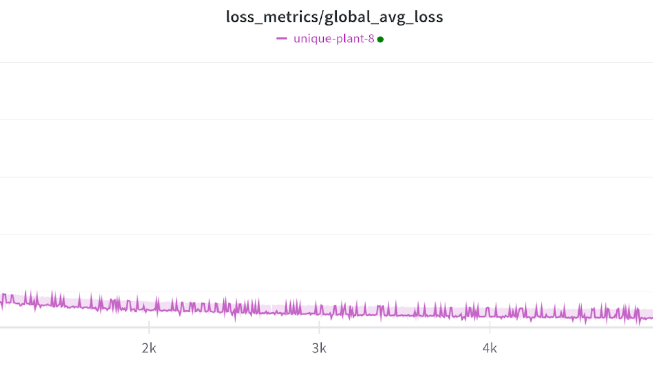
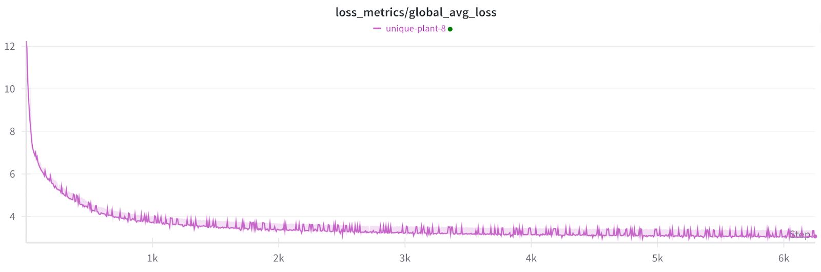
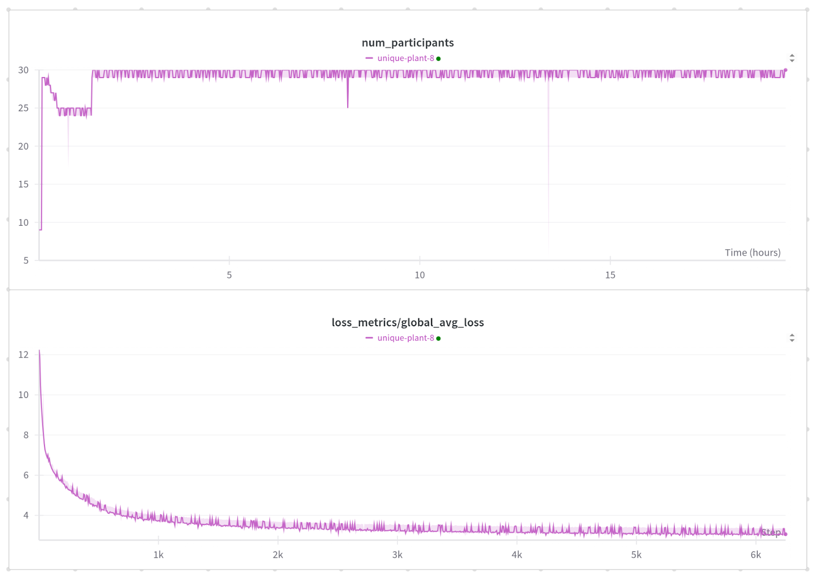
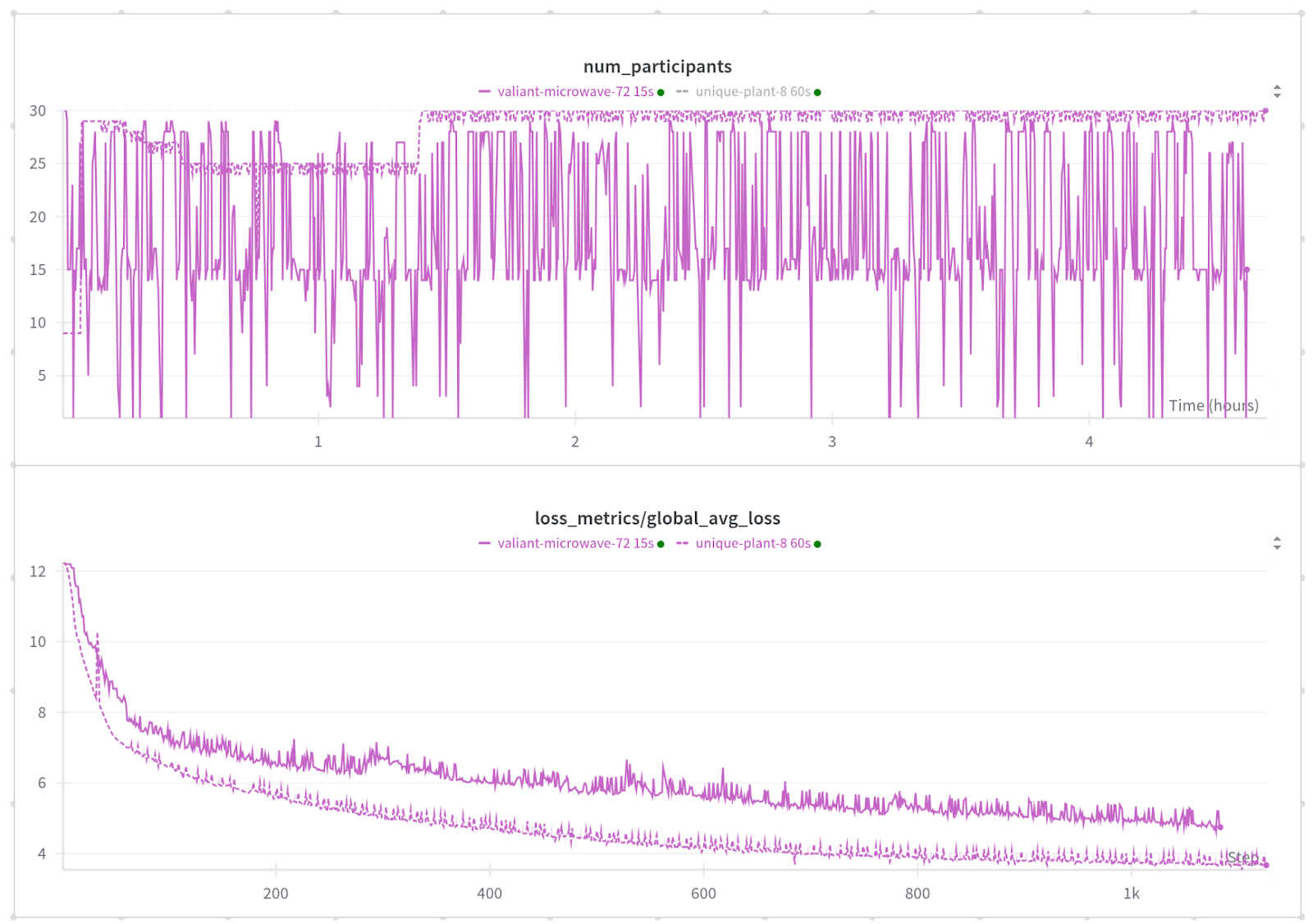
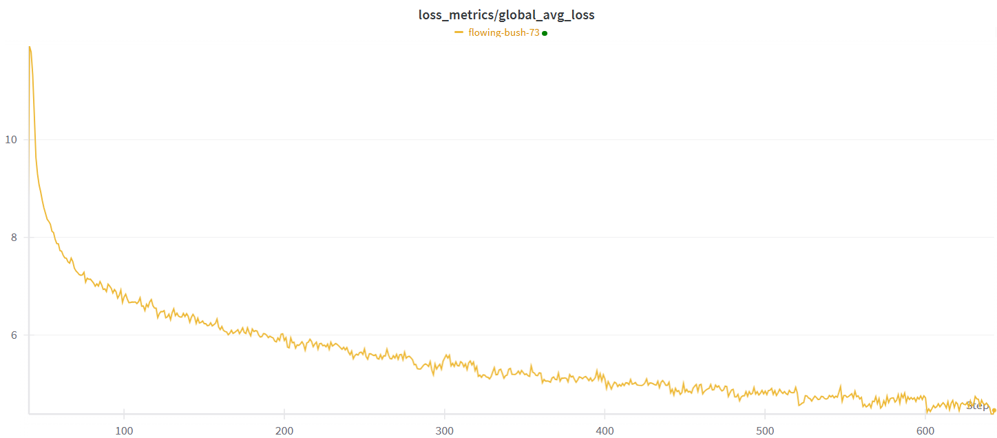
We did an integration test of Ghost Clipping DP-SGD with FSDP on an internal Meta use case, consisting of a Llama-3 8B model with LoRA fine-tuning for the next word prediction task. Our results show that Ghost Clipping with FSDP has roughly the same train loss (negligible difference) as DP-DDP. The previous results, as well as the unit test (link) have proved the correctness of the implementation.
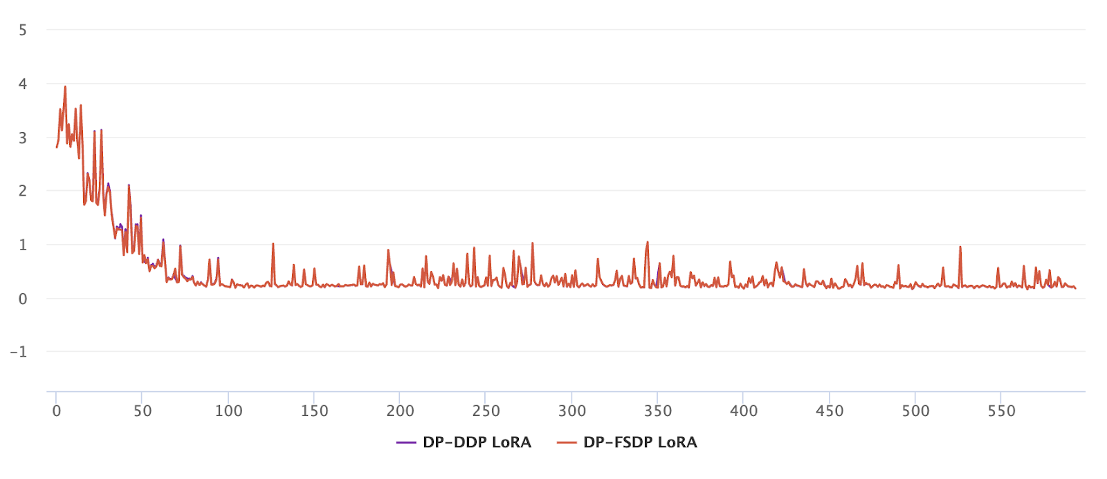
Figure 3: Training loss (y-axis) vs iterations (x-axis) for LoRA fine-tuning of Llama-3 8B using Ghost Clipping DP-SGD for next word prediction task.
Limitations
The current version of FSDP does not support the following scenarios:
- Layers with tied parameters.
- Freezing/unfreezing the trainable parameters within the training phase.
The following are the two main limitations with the current implementation of gradient accumulation with FSDP2 Ghost Clipping.
-
- Latency:
- The current implementation of gradient accumulation with FSDP2 synchronizes the gradients after every backward pass. Since Ghost Clipping has two backward passes, we have 2k gradient synchronization calls (reduce_scatter) for k gradient accumulation steps.
- This is because no_sync can’t be directly used when there are two backward passes for each forward pass.
- Ideally, we should have only 1 gradient synchronization call for k gradient accumulation steps.
- The latency of reduce_scatter is negligible in case of LoRA fine-tuning. Also, with a reasonable compute / communication overlap, this overhead can be masked.
- Latency:
- Memory:
-
- Gradient accumulation uses an additional buffer to store the accumulated gradients (sharded) irrespective of the number of gradient accumulation steps.
- We would like to avoid the usage of an additional buffer when the number of gradient accumulation steps is equal to one. This is not specific to FSDP2 and is a bottleneck for the Opacus library in general.
Main takeaway
- For models with small size of trainable parameters, e.g. LoRA fine-tuning
- It is recommended to use DP-DDP with gradient accumulation whenever possible.
- Shift to FSDP2 if DP-DDP throws an OOM error for the required sequence length or model size.
- For full fine-tuning with a reasonably large number of trainable parameters
- It is recommended to use FSDP2 as it has higher throughput than DP-DDP
- In most cases, FSDP2 is the only option as DP-DDP triggers OOM even with a batch size of one.
- The above observations hold for both private and non-private cases.
Conclusion
In this post, we present the integration of Fully Sharded Data Parallel (FSDP) with Fast Gradient Clipping (FGC) and Ghost Clipping (GC) in Opacus, demonstrating its potential to scale the private training of large-scale models with over 1 billion trainable parameters. By leveraging FSDP, we have shown that it is possible to fully fine-tune the Llama-3 8B model, a feat that is not achievable with Differentially Private Distributed Data Parallel (DP-DDP) due to memory constraints.
The introduction of FSDP in Opacus marks a significant advancement to the Opacus library, offering a scalable and memory-efficient solution for private training of LLMs. This development not only enhances the capability of Opacus to handle large-scale models but also sets the stage for future integration of other model parallelism strategies.
Looking ahead, our focus will be on enabling 2D parallelism with Ghost Clipping and integrating FSDP with native Opacus using hooks. These efforts aim to further optimize the training process, reduce latency, and expand the applicability of Opacus to even larger and more complex models. We are excited about the possibilities that these advancements will unlock and are committed to pushing the boundaries of what is possible in private machine learning. Furthermore, we invite developers, researchers, and enthusiasts to join us in this journey. Your contributions and insights are invaluable as we continue to enhance Opacus.


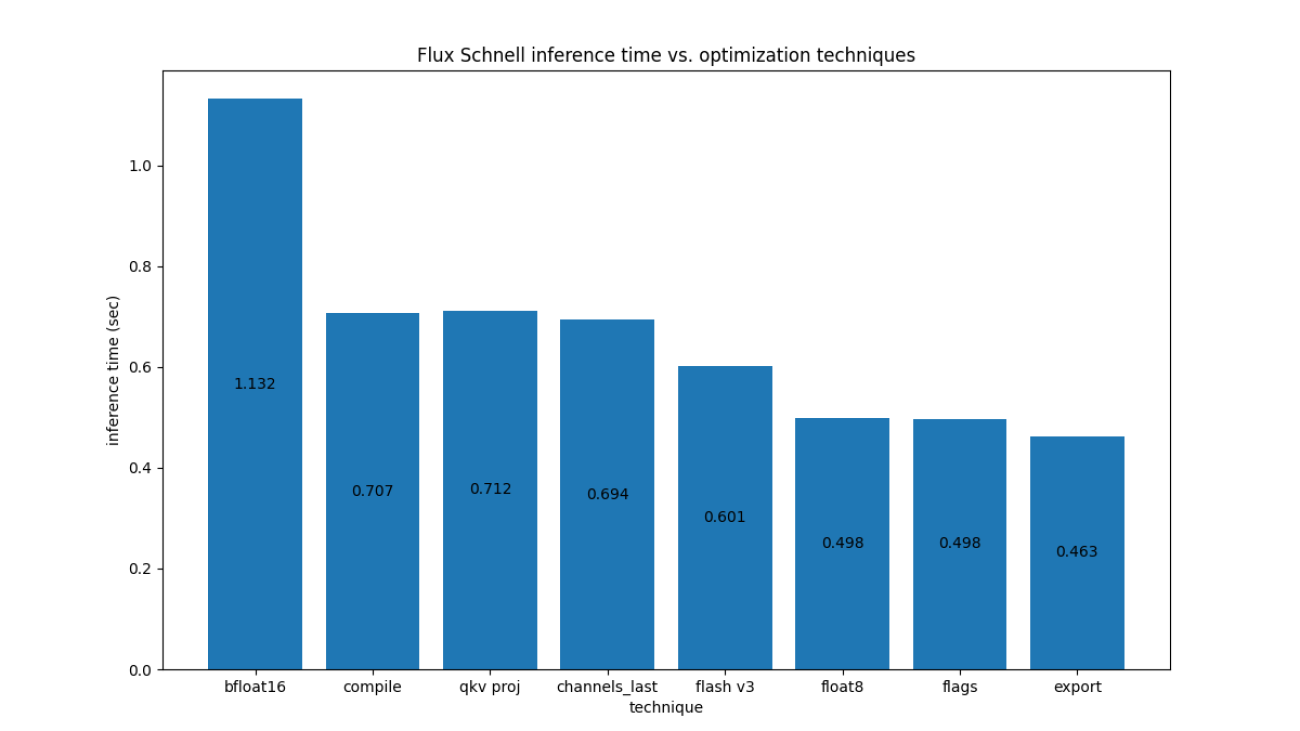
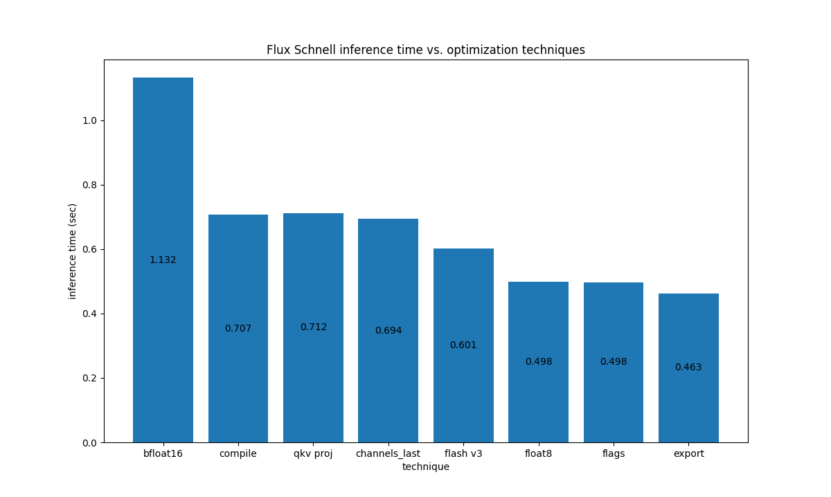 For Flux.1-Dev on H100, we have the following
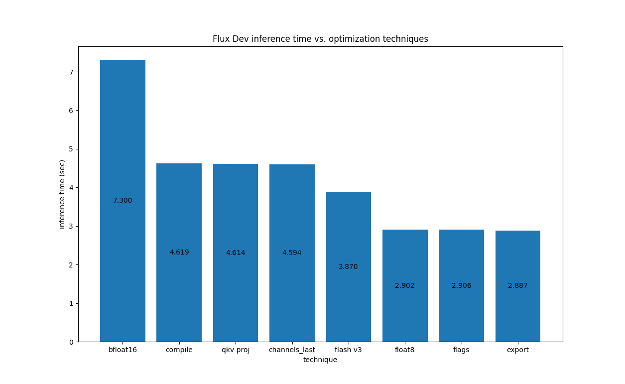


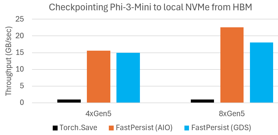
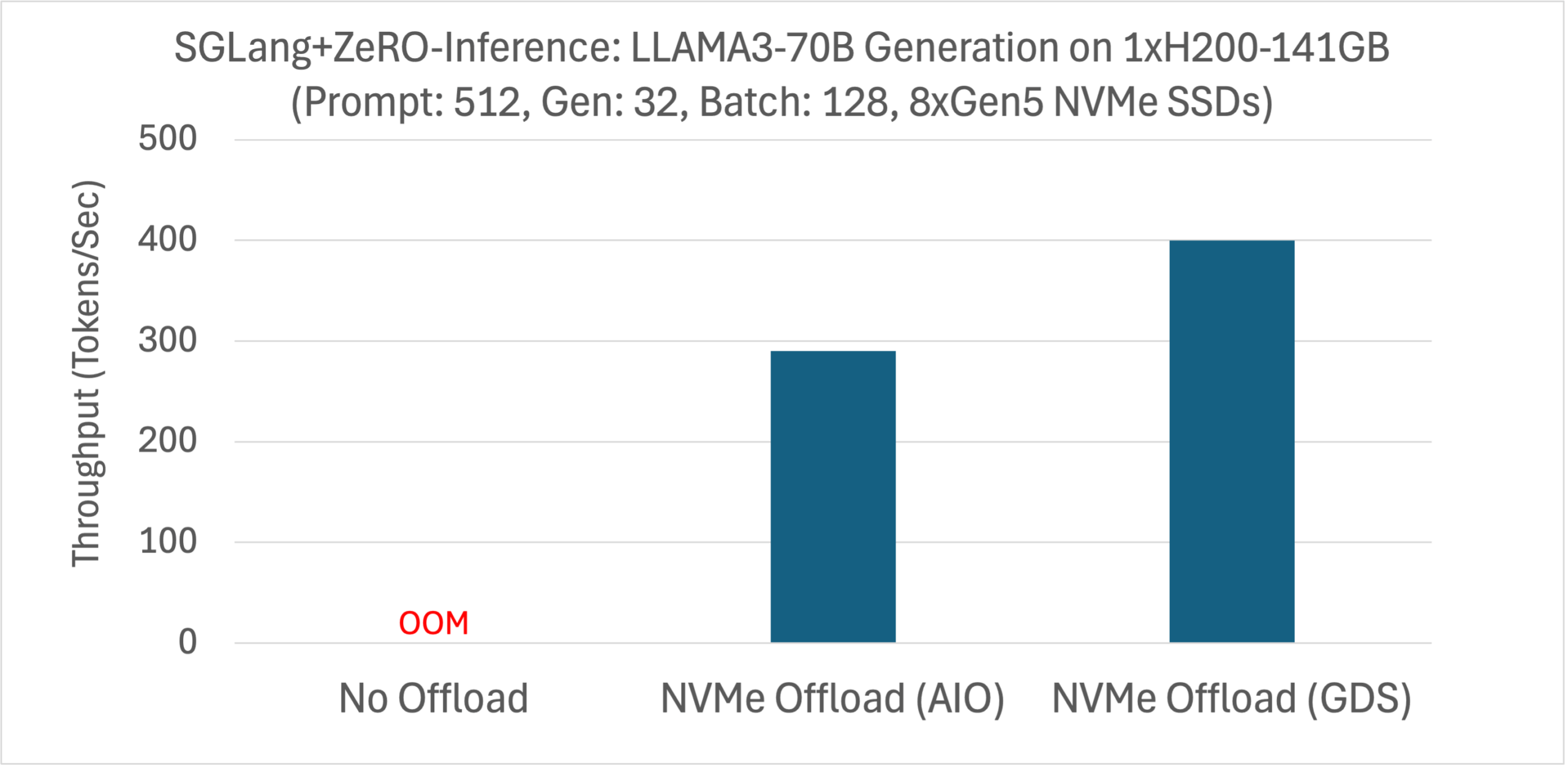
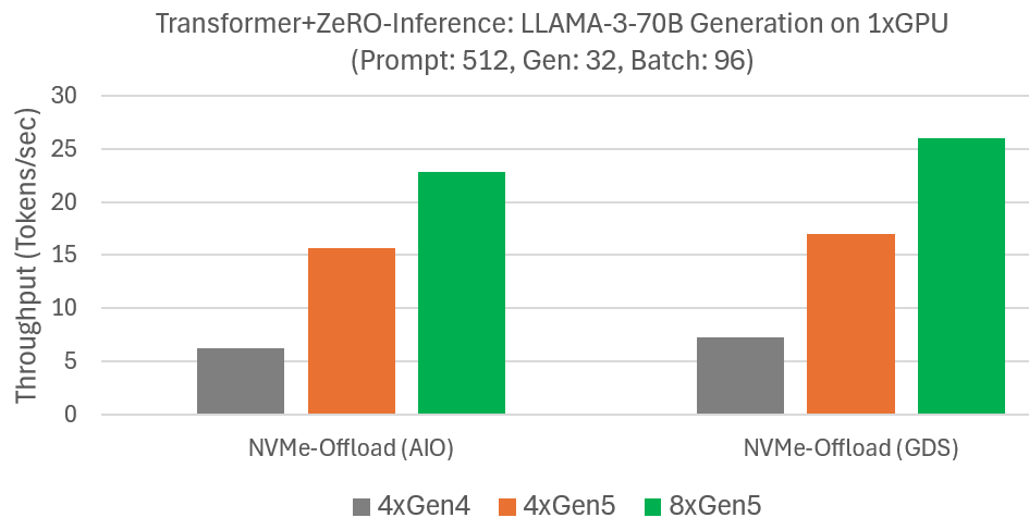
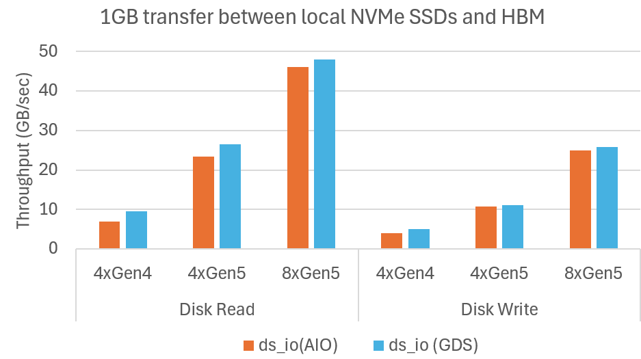 Microbenchmark shows DeepNVMe scales I/O performance with available NVMe bandwidth