Monthly Archives: December 2022

Last year, we announced the general availability of RStudio on Amazon SageMaker, the industry’s first fully managed RStudio Workbench integrated development environment (IDE) in the cloud. You can quickly launch the familiar RStudio IDE and dial up and down the underlying compute resources without interrupting your work, making it easy to build machine learning (ML) and analytics solutions in R at scale.

Many of the RStudio on SageMaker users are also users of Amazon Redshift, a fully managed, petabyte-scale, massively parallel data warehouse for data storage and analytical workloads. It makes it fast, simple, and cost-effective to analyze all your data using standard SQL and your existing business intelligence (BI) tools. Users can also interact with data with ODBC, JDBC, or the Amazon Redshift Data API.

The use of RStudio on SageMaker and Amazon Redshift can be helpful for efficiently performing analysis on large data sets in the cloud. However, working with data in the cloud can present challenges, such as the need to remove organizational data silos, maintain security and compliance, and reduce complexity by standardizing tooling. AWS offers tools such as RStudio on SageMaker and Amazon Redshift to help tackle these challenges.

In this blog post, we will show you how to use both of these services together to efficiently perform analysis on massive data sets in the cloud while addressing the challenges mentioned above. This blog focuses on the Rstudio on Amazon SageMaker language, with business analysts, data engineers, data scientists, and all developers that use the R Language and Amazon Redshift, as the target audience.

If you’d like to use the traditional SageMaker Studio experience with Amazon Redshift, refer to Using the Amazon Redshift Data API to interact from an Amazon SageMaker Jupyter notebook.

Solution overview

In the blog today, we will be executing the following steps:

1. Cloning the sample repository with the required packages.
2. Connecting to Amazon Redshift with a secure ODBC connection (ODBC is the preferred protocol for RStudio).
3. Running queries and SageMaker API actions on data within Amazon Redshift Serverless through RStudio on SageMaker

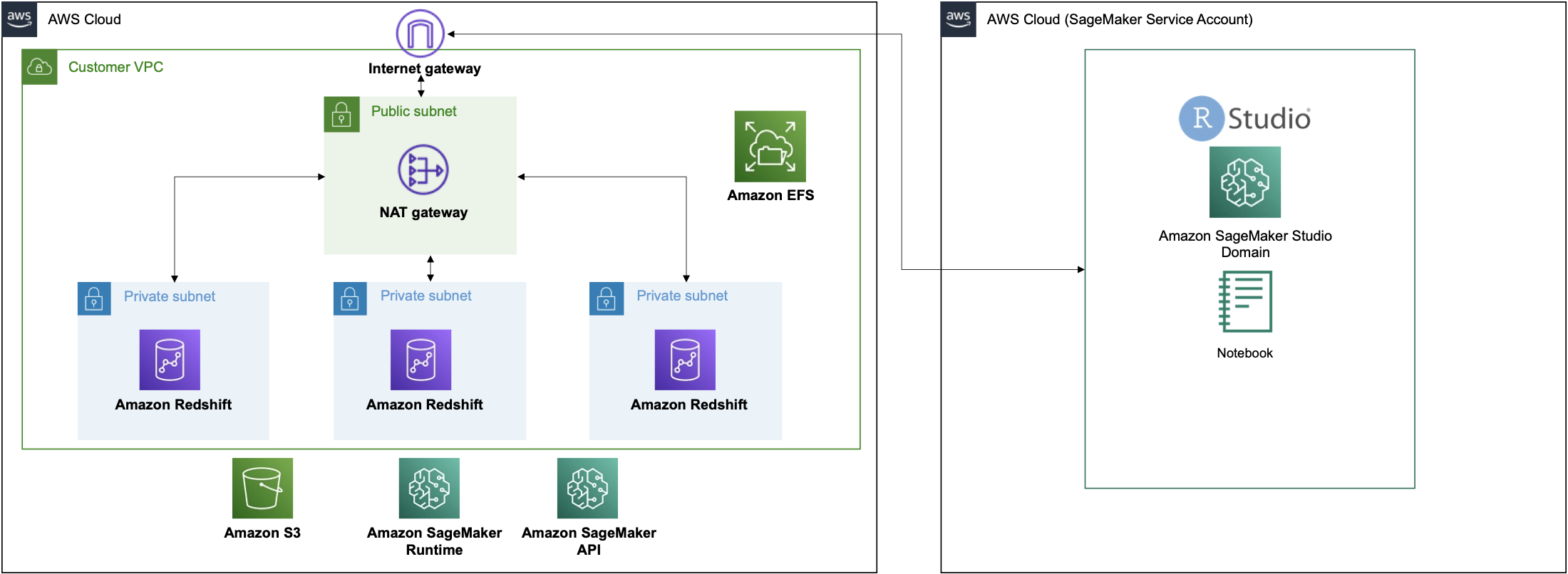
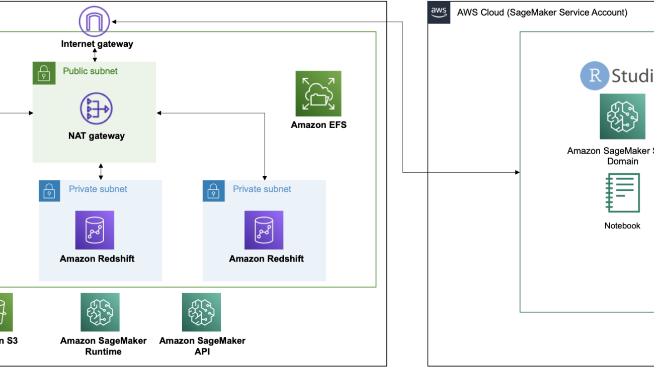
This process is depicted in the following solutions architecture:

Solution walkthrough

Prerequisites

Prior to getting started, ensure you have all requirements for setting up RStudio on Amazon SageMaker and Amazon Redshift Serverless, such as:

• The correct IAM permissions
• RStudio Workbench license

We will be using a CloudFormation stack to generate the required infrastructure.

Note: If you already have an RStudio domain and Amazon Redshift cluster you can skip this step

Launching this stack creates the following resources:

• 3 Private subnets
• 1 Public subnet
• 1 NAT gateway
• Internet gateway
• Amazon Redshift Serverless cluster
• SageMaker domain with RStudio
• SageMaker RStudio user profile
• IAM service role for SageMaker RStudio domain execution
• IAM service role for SageMaker RStudio user profile execution

This template is designed to work in a Region (ex. us-east-1, us-west-2) with three Availability Zones, RStudio on SageMaker, and Amazon Redshift Serverless. Ensure your Region has access to those resources, or modify the templates accordingly.

Press the Launch Stack button to create the stack.

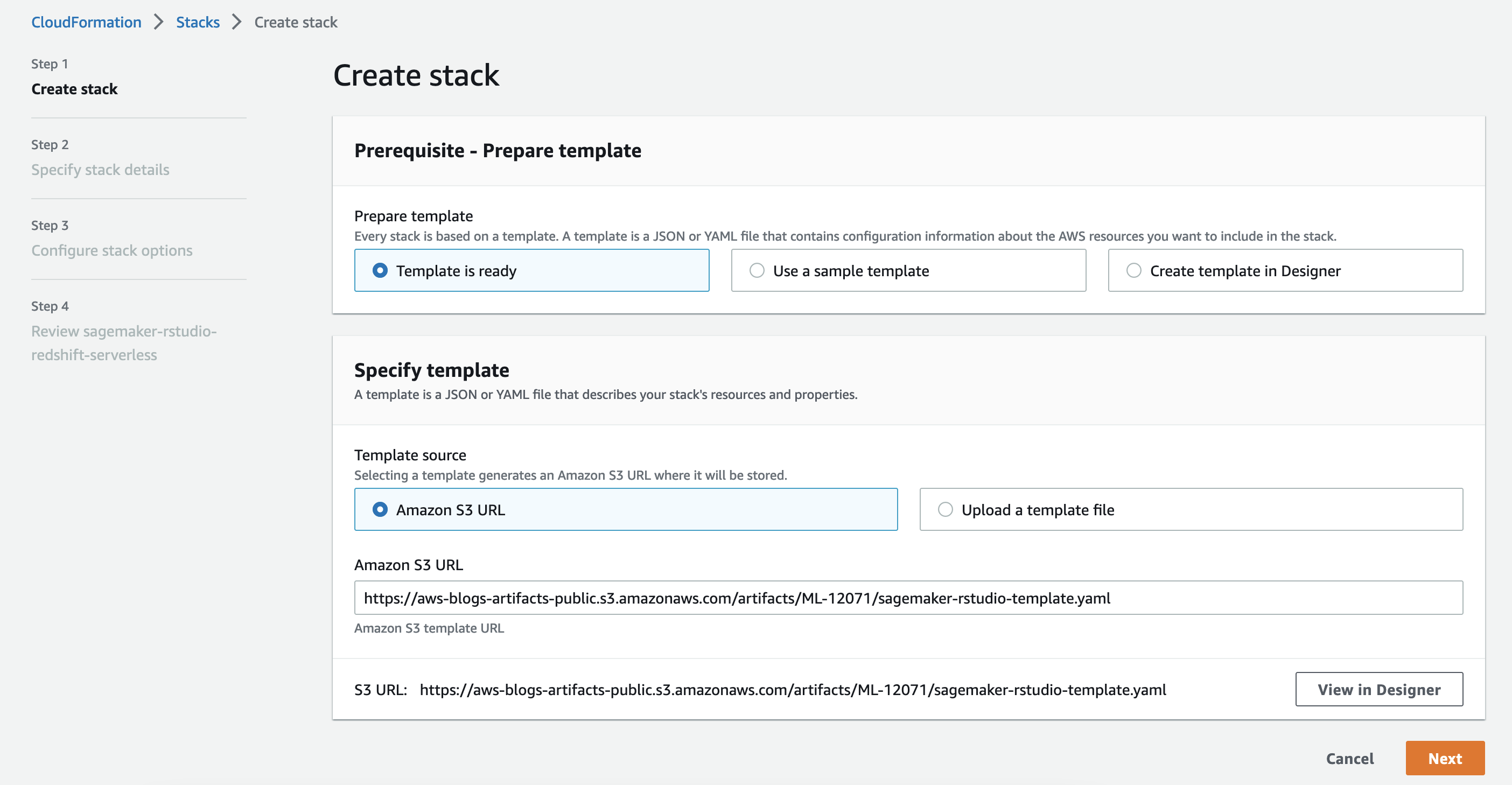
1. On the Create stack page, choose Next.
2. On the Specify stack details page, provide a name for your stack and leave the remaining options as default, then choose Next.
3. On the Configure stack options page, leave the options as default and press Next.
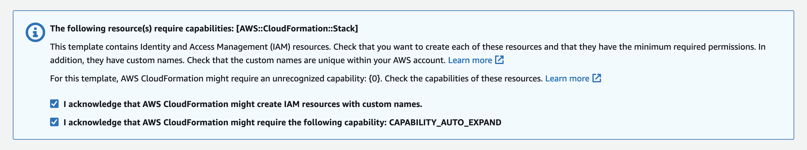
4. On the Review page, select the

• I acknowledge that AWS CloudFormation might create IAM resources with custom names
• I acknowledge that AWS CloudFormation might require the following capability: CAPABILITY_AUTO_EXPANDcheckboxes and choose Submit.

The template will generate five stacks.

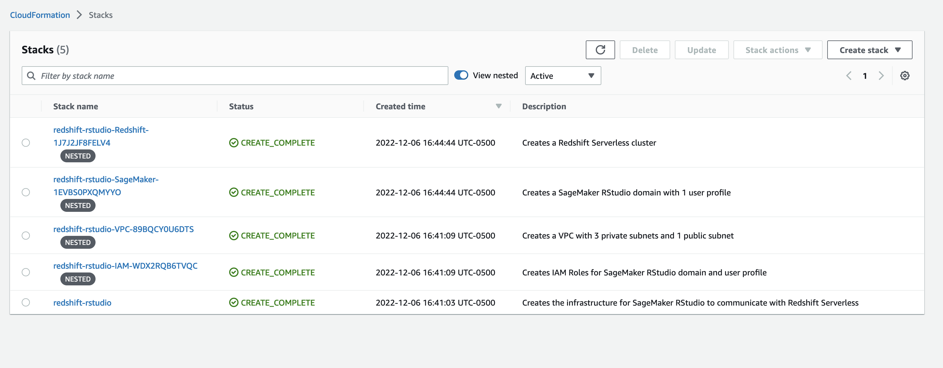
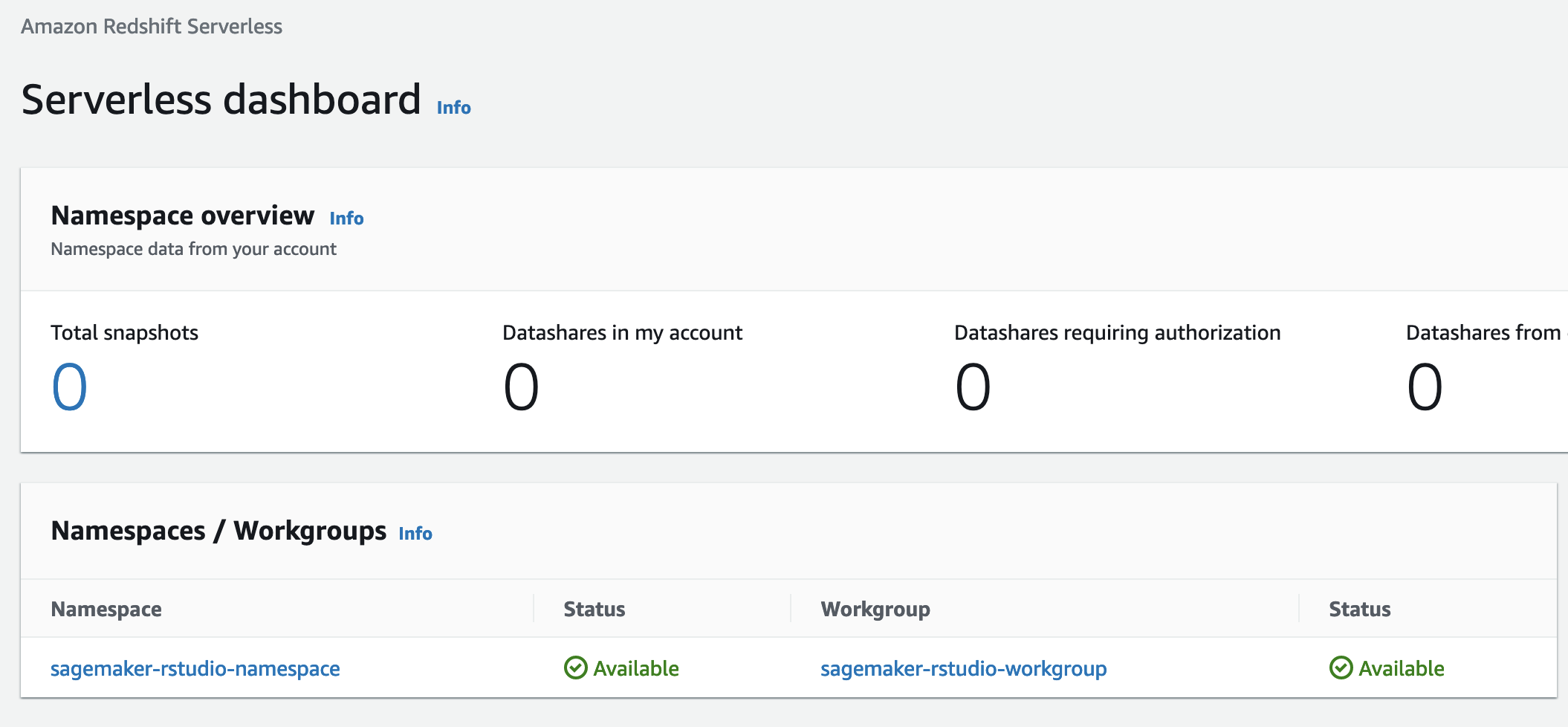
Once the stack status is CREATE_COMPLETE, navigate to the Amazon Redshift Serverless console. This is a new capability that makes it super easy to run analytics in the cloud with high performance at any scale. Just load your data and start querying. There is no need to set up and manage clusters.

Note: The pattern demonstrated in this blog integrating Amazon Redshift and RStudio on Amazon SageMaker will be the same regardless of Amazon Redshift deployment pattern (serverless or traditional cluster).

Loading data in Amazon Redshift Serverless

The CloudFormation script created a database called sagemaker. Let’s populate this database with tables for the RStudio user to query. Create a SQL editor tab and be sure the sagemaker database is selected. We will be using the synthetic credit card transaction data to create tables in our database. This data is part of the SageMaker sample tabular datasets s3://sagemaker-sample-files/datasets/tabular/synthetic_credit_card_transactions.

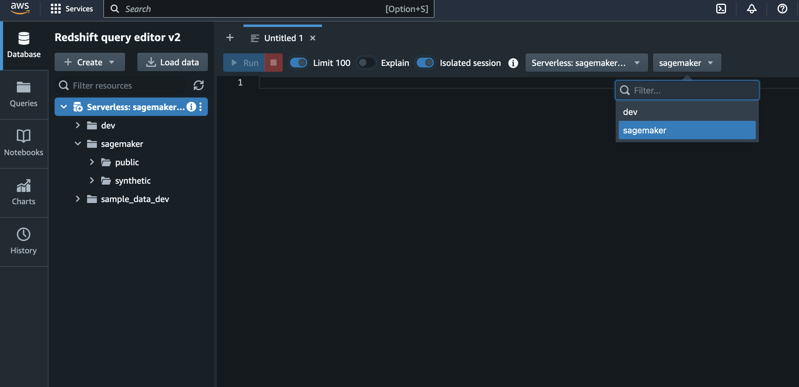
We are going to execute the following query in the query editor. This will generate three tables, cards, transactions, and users.

CREATE SCHEMA IF NOT EXISTS synthetic;
DROP TABLE IF EXISTS synthetic.transactions;

CREATE TABLE synthetic.transactions(
    user_id INT,
    card_id INT,
    year INT,
    month INT,
    day INT,
    time_stamp TIME,
    amount VARCHAR(100),
    use_chip VARCHAR(100),
    merchant_name VARCHAR(100),
    merchant_city VARCHAR(100),
    merchant_state VARCHAR(100),
    merchant_zip_code VARCHAR(100),
    merchant_category_code INT,
    is_error VARCHAR(100),
    is_fraud VARCHAR(100)
);

COPY synthetic.transactions
FROM 's3://sagemaker-sample-files/datasets/tabular/synthetic_credit_card_transactions/credit_card_transactions-ibm_v2.csv'
IAM_ROLE default
REGION 'us-east-1' 
IGNOREHEADER 1 
CSV;

DROP TABLE IF EXISTS synthetic.cards;

CREATE TABLE synthetic.cards(
    user_id INT,
    card_id INT,
    card_brand VARCHAR(100),
    card_type VARCHAR(100),
    card_number VARCHAR(100),
    expire_date VARCHAR(100),
    cvv INT,
    has_chip VARCHAR(100),
    number_cards_issued INT,
    credit_limit VARCHAR(100),
    account_open_date VARCHAR(100),
    year_pin_last_changed VARCHAR(100),
    is_card_on_dark_web VARCHAR(100)
);

COPY synthetic.cards
FROM 's3://sagemaker-sample-files/datasets/tabular/synthetic_credit_card_transactions/sd254_cards.csv'
IAM_ROLE default
REGION 'us-east-1' 
IGNOREHEADER 1 
CSV;

DROP TABLE IF EXISTS synthetic.users;

CREATE TABLE synthetic.users(
    name VARCHAR(100),
    current_age INT,
    retirement_age INT,
    birth_year INT,
    birth_month INT,
    gender VARCHAR(100),
    address VARCHAR(100),
    apartment VARCHAR(100),
    city VARCHAR(100),
    state VARCHAR(100),
    zip_code INT,
    lattitude VARCHAR(100),
    longitude VARCHAR(100),
    per_capita_income_zip_code VARCHAR(100),
    yearly_income VARCHAR(100),
    total_debt VARCHAR(100),
    fico_score INT,
    number_credit_cards INT
);

COPY synthetic.users
FROM 's3://sagemaker-sample-files/datasets/tabular/synthetic_credit_card_transactions/sd254_users.csv'
IAM_ROLE default
REGION 'us-east-1' 
IGNOREHEADER 1 
CSV;

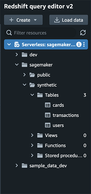
You can validate that the query ran successfully by seeing three tables within the left-hand pane of the query editor.

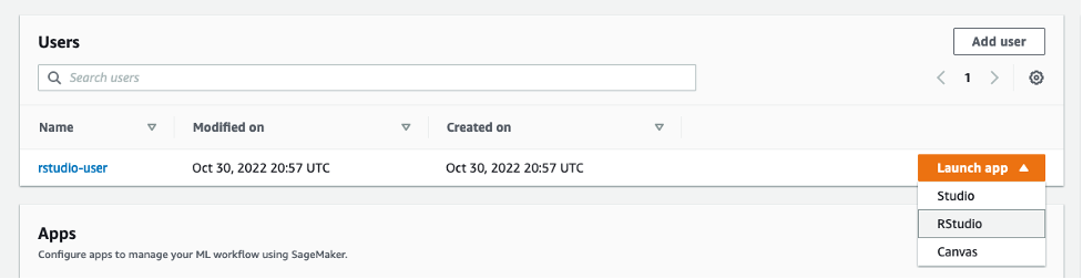
Once all of the tables are populated, navigate to SageMaker RStudio and start a new session with RSession base image on an ml.m5.xlarge instance.

Once the session is launched, we will run this code to create a connection to our Amazon Redshift Serverless database.

library(DBI)
library(reticulate)
boto3 <- import('boto3')
client <- boto3$client('redshift-serverless')
workgroup <- unlist(client$list_workgroups())
namespace <- unlist(client$get_namespace(namespaceName=workgroup$workgroups.namespaceName))
creds <- client$get_credentials(dbName=namespace$namespace.dbName,
                                durationSeconds=3600L,
                                workgroupName=workgroup$workgroups.workgroupName)
con <- dbConnect(odbc::odbc(),
                 Driver='redshift',
                 Server=workgroup$workgroups.endpoint.address,
                 Port='5439',
                 Database=namespace$namespace.dbName,
                 UID=creds$dbUser,
                 PWD=creds$dbPassword)

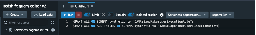
In order to view the tables in the synthetic schema, you will need to grant access in Amazon Redshift via the query editor.

GRANT ALL ON SCHEMA synthetic to "IAMR:SageMakerUserExecutionRole";
GRANT ALL ON ALL TABLES IN SCHEMA synthetic to "IAMR:SageMakerUserExecutionRole";

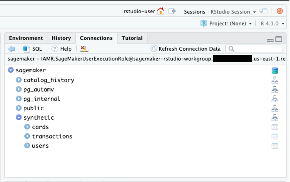
The RStudio Connections pane should show the sagemaker database with schema synthetic and tables cards, transactions, users.

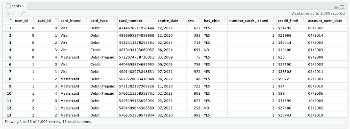
You can click the table icon next to the tables to view 1,000 records.

Note: We have created a pre-built R Markdown file with all the code-blocks pre-built that can be found at the project GitHub repo.

Now let’s use the DBI package function dbListTables() to view existing tables.

dbListTables(con)

Use dbGetQuery() to pass a SQL query to the database.

dbGetQuery(con, "select * from synthetic.users limit 100")
dbGetQuery(con, "select * from synthetic.cards limit 100")
dbGetQuery(con, "select * from synthetic.transactions limit 100")

We can also use the dbplyr and dplyr packages to execute queries in the database. Let’s count() how many transactions are in the transactions table. But first, we need to install these packages.

install.packages(c("dplyr", "dbplyr", "crayon"))

Use the tbl() function while specifying the schema.

library(dplyr)
library(dbplyr)

users_tbl <- tbl(con, in_schema("synthetic", "users"))
cards_tbl <- tbl(con, in_schema("synthetic", "cards"))
transactions_tbl <- tbl(con, in_schema("synthetic", "transactions"))

Let’s run a count of the number of rows for each table.

count(users_tbl)
count(cards_tbl)
count(transactions_tbl)

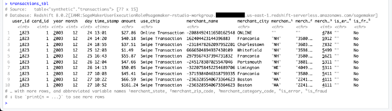
So we have 2,000 users; 6,146 cards; and 24,386,900 transactions. We can also view the tables in the console.

transactions_tbl

We can also view what dplyr verbs are doing under the hood.

show_query(transactions_tbl)

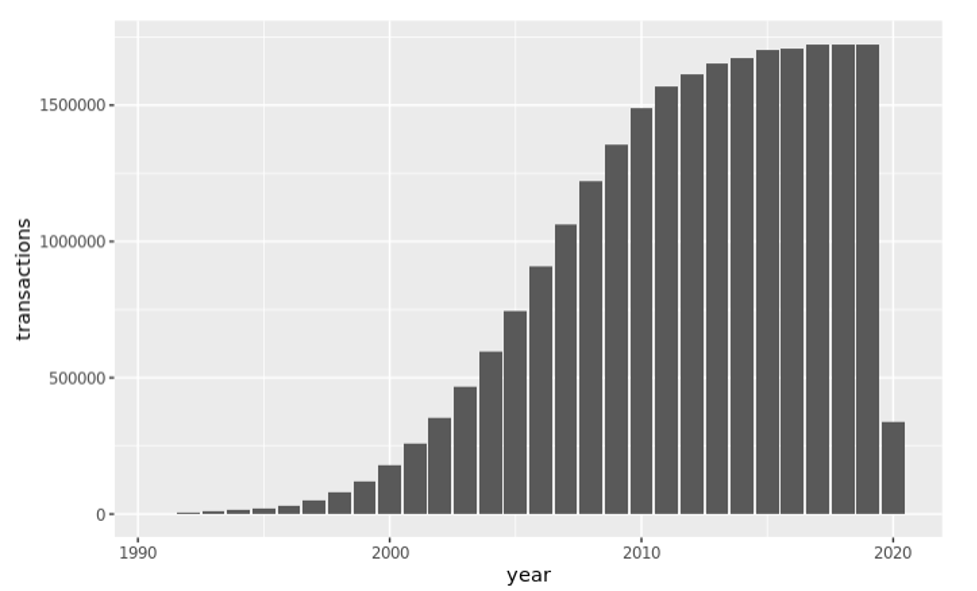
Let’s visually explore the number of transactions by year.

transactions_by_year <- transactions_tbl %>%
  count(year) %>%
  arrange(year) %>%
  collect()

transactions_by_year
install.packages(c('ggplot2', 'vctrs'))
library(ggplot2)
ggplot(transactions_by_year) +
  geom_col(aes(year, as.integer(n))) +
  ylab('transactions') 

We can also summarize data in the database as follows:

transactions_tbl %>%
  group_by(is_fraud) %>%
  count()
transactions_tbl %>%
  group_by(merchant_category_code, is_fraud) %>%
  count() %>% 
  arrange(merchant_category_code)

Suppose we want to view fraud using card information. We just need to join the tables and then group them by the attribute.

cards_tbl %>%
  left_join(transactions_tbl, by = c("user_id", "card_id")) %>%
  group_by(card_brand, card_type, is_fraud) %>%
  count() %>% 
  arrange(card_brand)

Now let’s prepare a dataset that could be used for machine learning. Let’s filter the transaction data to just include Discover credit cards while only keeping a subset of columns.

discover_tbl <- cards_tbl %>%
  filter(card_brand == 'Discover', card_type == 'Credit') %>%
  left_join(transactions_tbl, by = c("user_id", "card_id")) %>%
  select(user_id, is_fraud, merchant_category_code, use_chip, year, month, day, time_stamp, amount)

And now let’s do some cleaning using the following transformations:

• Convert is_fraud to binary attribute
• Remove transaction string from use_chip and rename it to type
• Combine year, month, and day into a data object
• Remove $ from amount and convert to a numeric data type

discover_tbl <- discover_tbl %>%
  mutate(is_fraud = ifelse(is_fraud == 'Yes', 1, 0),
         type = str_remove(use_chip, 'Transaction'),
         type = str_trim(type),
         type = tolower(type),
         date = paste(year, month, day, sep = '-'),
         date = as.Date(date),
         amount = str_remove(amount, '[$]'),
         amount = as.numeric(amount)) %>%
  select(-use_chip, -year, -month, -day)

Now that we have filtered and cleaned our dataset, we are ready to collect this dataset into local RAM.

discover <- collect(discover_tbl)
summary(discover)

Now we have a working dataset to start creating features and fitting models. We will not cover those steps in this blog, but if you want to learn more about building models in RStudio on SageMaker refer to Announcing Fully Managed RStudio on Amazon SageMaker for Data Scientists.

Cleanup

To clean up any resources to avoid incurring recurring costs, delete the root CloudFormation template. Also delete all EFS mounts created and any S3 buckets and objects created.

Conclusion

Data analysis and modeling can be challenging when working with large datasets in the cloud. Amazon Redshift is a popular data warehouse that can help users perform these tasks. RStudio, one of the most widely used integrated development environments (IDEs) for data analysis, is often used with R language. In this blog post, we showed how to use Amazon Redshift and RStudio on SageMaker together to efficiently perform analysis on massive datasets. By using RStudio on SageMaker, users can take advantage of the fully managed infrastructure, access control, networking, and security capabilities of SageMaker, while also simplifying integration with Amazon Redshift. If you would like to learn more about using these two tools together, check out our other blog posts and resources. You can also try using RStudio on SageMaker and Amazon Redshift for yourself and see how they can help you with your data analysis and modeling tasks.

Please add your feedback to this blog, or create a pull request on the GitHub.

About the Authors

Ryan Garner is a Data Scientist with AWS Professional Services. He is passionate about helping AWS customers use R to solve their Data Science and Machine Learning problems.

Raj Pathak is a Senior Solutions Architect and Technologist specializing in Financial Services (Insurance, Banking, Capital Markets) and Machine Learning. He specializes in Natural Language Processing (NLP), Large Language Models (LLM) and Machine Learning infrastructure and operations projects (MLOps).

Aditi Rajnish is a Second-year software engineering student at University of Waterloo. Her interests include computer vision, natural language processing, and edge computing. She is also passionate about community-based STEM outreach and advocacy. In her spare time, she can be found rock climbing, playing the piano, or learning how to bake the perfect scone.

Saiteja Pudi is a Solutions Architect at AWS, based in Dallas, Tx. He has been with AWS for more than 3 years now, helping customers derive the true potential of AWS by being their trusted advisor. He comes from an application development background, interested in Data Science and Machine Learning.

Read More

The last decade of the Industry 4.0 revolution has shown the value and importance of machine learning (ML) across verticals and environments, with more impact on manufacturing than possibly any other application. Organizations implementing a more automated, reliable, and cost-effective Operational Technology (OT) strategy have led the way, recognizing the benefits of ML in predicting assembly line failures to avoid costly and unplanned downtime. Still, challenges remain for teams of all sizes to quickly, and with little effort, demonstrate the value of ML-based anomaly detection in order to persuade management and finance owners to allocate the budget required to implement these new technologies. Without access to data scientists for model training, or ML specialists to deploy solutions at the local level, adoption has seemed out of reach for teams on the factory floor.

Now, teams that collect sensor data signals from machines in the factory can unlock the power of services like Amazon Timestream, Amazon Lookout for Equipment, and AWS IoT Core to easily spin up and test a fully production-ready system at the local edge to help avoid catastrophic downtime events. Lookout for Equipment uses your unique ML model to analyze incoming sensor data in real time and accurately identify early warning signs that could lead to machine failures. This means you can detect equipment abnormalities with speed and precision, quickly diagnose issues, take action to reduce expensive downtime, and reduce false alerts. Response teams can be alerted with specific pinpoints to which sensors are indicating the issue, and the magnitude of impact on the detected event.

In this post, we show you how you can set up a system to simulate events on your factory floor with a trained model and detect abnormal behavior using Timestream, Lookout for Equipment, and AWS Lambda functions. The steps in this post emphasize the AWS Management Console UI, showing how technical people without a developer background or strong coding skills can build a prototype. Using simulated sensor signals will allow you to test your system and gain confidence before cutting over to production. Lastly, in this example, we use Amazon Simple Notification Service (Amazon SNS) to show how teams can receive notifications of predicted events and respond to avoid catastrophic effects of assembly line failures. Additionally, teams can use Amazon QuickSight for further analysis and dashboards for reporting.

Solution overview

To get started, we first collect a historical dataset from your factory sensor readings, ingest the data, and train the model. With the trained model, we then set up IoT Device Simulator to publish MQTT signals to a topic that will allow testing of the system to identify desired production settings before production data is used, keeping costs low.

The following diagram illustrates our solution architecture.

The workflow contains the following steps:

1. Use sample data to train the Lookout for Equipment model, and the provided labeled data to improve model accuracy. With a sample rate of 5 minutes, we can train the model in 20–30 minutes.
2. Run an AWS CloudFormation template to enable IoT Simulator, and create a simulation to publish an MQTT topic in the format of the sensor data signals.
3. Create an IoT rule action to read the MQTT topic an send the topic payload to Timestream for storage. These are the real-time datasets that will be used for inferencing with the ML model.
4. Set up a Lambda function triggered by Amazon EventBridge to convert data into CSV format for Lookout for Equipment.
5. Create a Lambda function to parse Lookout for Equipment model inferencing output file in Amazon Simple Storage Service (Amazon S3) and, if failure is predicted, send an email to the configured address. Additionally, use AWS Glue, Amazon Athena, and QuickSight to visualize the sensor data contributions to the predicted failure event.

Prerequisites

You need access to an AWS account to set up the environment for anomaly detection.

Simulate data and ingest it into the AWS Cloud

To set up your data and ingestion configuration, complete the following steps:

1. Download the training file subsystem-08_multisensor_training.csv and the labels file labels_data.csv. Save the files locally.
2. On the Amazon S3 console in your preferred Region, create a bucket with a unique name (for example, l4e-training-data), using the default configuration options.
3. Open the bucket and choose Upload, then Add files.
   
4. Upload the training data to a folder called /training-data and the label data to a folder called /labels.

Next, you create the ML model to be trained with the data from the S3 bucket. To do this, you first need to create a project.

5. On the Lookout for Equipment console, choose Create project.
   
6. Name the project and choose Create project.
7. On the Add dataset page, specify your S3 bucket location.
8. Use the defaults for Create a new role and Enable CloudWatch Logs.
9. Choose By filename for Schema detection method.
10. Choose Start ingestion.

Ingestion takes a few minutes to complete.

11. When ingestion is complete, you can review the details of the dataset by choosing View Dataset.
12. Scroll down the page and review the Details by sensor section.
13. Scroll to the bottom of the page to see that the sensor grade for data from three of the sensors is labeled Low.
14. Select all the sensor records except the three with Low grade.
15. Choose Create model.
    
16. On the Specify model details page, give the model a name and choose Next.
17. On the Configure input data page, enter values for the training and evaluation settings and a sample rate (for this post, 1 minute).
18. Skip the Off-time detection settings and choose Next.
    
19. On the Provide data labels page, specify the S3 folder location where the label data is.
20. Select Create a new role.
21. Choose Next.
    
22. On the Review and train page, choose Start training.

With a sample rate of 5 minutes, the model should take 20–30 minutes to build.

While the model is building, we can set up the rest of the architecture.

Simulate sensor data

1. Choose Launch Stack to launch a CloudFormation template to set up the simulated sensor signals using IoT Simulator.
2. After the template has launched, navigate to the CloudFormation console.
3. On the Stacks page, choose IoTDeviceSimulator to see the stack details.
4. On the Outputs tab, find the ConsoleURL key and the corresponding URL value.
   
5. Choose the URL to open the IoT Device Simulator login page.
6. Create a user name and password and choose SIGN IN.
7. Save your credentials in case you need to sign in again later.
   
8. From the IoT Device Simulator menu bar, choose Device Types.
9. Enter a device type name, such as My_testing_device.
10. Enter an MQTT topic, such as factory/line/station/simulated_testing.
11. Choose Add attribute.
    
12. Enter the values for the attribute signal5, as shown in the following screenshot.
13. Choose Save.
    
14. Choose Add attribute again and add the remaining attributes to match the sample signal data, as shown in the following table.

15. On the Simulations tab, choose Add Simulation.
16. Give the simulation a name.
17. Specify Simulation type as User created, Device type as the recently created device, Data transmission interval as 60, and Data transmission duration as 3600.
18. Finally, start the simulation you just created and see the payloads generated on the Simulation Details page by choosing View.

Now that signals are being generated, we can set up IoT Core to read the MQTT topics and direct the payloads to the Timestream database.

19. On the IoT Core console, under Message Routing in the navigation pane, choose Rules.
20. Choose Create rule.
21. Enter a rule name and choose Next.
22. Enter the following SQL statement to pull all the values from the published MQTT topic:

SELECT signal5, signal6, signal7, signal8, signal48, signal49, signal78, signal109, signal120, signal121 FROM 'factory/line/station/simulated_testing'

23. Choose Next.
24. For Rule actions, search for the Timestream table.
25. Choose Create Timestream database.

A new tab opens with the Timestream console.

26. Select Standard database.
27. Name the database sampleDB and choose Create database.

You’re redirected to the Timestream console, where you can view the database you created.

28. Return to the IoT Core tab and choose sampleDB for Database name.
29. Choose Create Timestream table to add a table to the database where the sensor data signals will be stored.
30. On the Timestream console Create table tab, choose sampleDB for Database name, enter signalTable for Table name, and choose Create table.
31. Return to the IoT Core console tab to complete the IoT message routing rule.
32. Enter Simulated_signal for Dimensions name and 1 for Dimensions value, then choose Create new role.

33. Name the role TimestreamRole and choose Next.
34. On the Review and create page, choose Create.

You have now added a rule action in IoT Core that directs the data published to the MQTT topic to a Timestream database.

Query Timestream for analysis

To query Timestream for analysis, complete the following steps:

1. Validate the data is being stored in the database by navigating to the Timestream console and choosing Query Editor.
2. Choose Select table, then choose the options menu and Preview data.
3. Choose Run to query the table.

Now that data is being stored in the stream, you can use Lambda and EventBridge to pull data every 5 minutes from the table, format it, and send it to Lookout for Equipment for inference and prediction results.

4. On the Lambda console, choose Create function.
5. For Runtime, choose Python 3.9.
6. For Layer source, select Specify an ARN.
7. Enter the correct ARN for your Region from the aws pandas resource.
8. Choose Add.

9. Enter the following code into the function and edit it to match the S3 path to a bucket with the folder /input (create a bucket folder for these data stream files if not already present).

This code uses the awswrangler library to easily format the data in the required CSV form needed for Lookout for Equipment. The Lambda function also dynamically names the data files as required.

import json
import boto3
import awswrangler as wr
from datetime import datetime
import pytz

def lambda_handler(event, context):
    # TODO implement
    UTC = pytz.utc
    my_date = datetime.now(UTC).strftime('%Y-%m-%d-%H-%M-%S')
    print(my_date)
      
    df = wr.timestream.query('SELECT time as Timestamp, max(case when measure_name = 'signal5' then measure_value::double/1000 end) as "signal-005", max(case when measure_name = 'signal6' then measure_value::double/1000 end) as "signal-006", max(case when measure_name = 'signal7' then measure_value::double/1000 end) as "signal-007", max(case when measure_name = 'signal8' then measure_value::double/1000 end) as "signal-008", max(case when measure_name = 'signal48' then measure_value::double/1000 end) as "signal-048", max(case when measure_name = 'signal49' then measure_value::double/1000 end) as "signal-049", max(case when measure_name = 'signal78' then measure_value::double/1000 end) as "signal-078", max(case when measure_name = 'signal109' then measure_value::double/1000 end) as "signal-109", max(case when measure_name = 'signal120' then measure_value::double/1000 end) as "signal-120", max(case when measure_name = 'signal121' then measure_value::double/1000 end) as "signal-121" 
    FROM "<YOUR DB NAME>"."<YOUR TABLE NAME>" WHERE time > ago(5m) group by time order by time desc')
    print(df)
    
    s3path ="s3://<EDIT-PATH-HERE>/input/<YOUR FILE NAME>_%s.csv" % my_date
    
    wr.s3.to_csv(df, s3path, index=False)
    
    return {
        'statusCode': 200,
        'body': json.dumps('Hello from Lambda!')
    }

10. Choose Deploy.
11. On the Configuration tab, choose General configuration.
12. For Timeout, choose 5 minutes.
13. In the Function overview section, choose Add trigger with EventBridge as the source.
14. Select Create a new rule.
15. Name the rule eventbridge-cron-job-lambda-read-timestream and add rate(5 minutes) for Schedule expression.
16. Choose Add.
    
17. Add the following policy to your Lambda execution role:

    {
        "Version": "2012-10-17",
        "Statement": [
            {
                "Effect": "Allow",
                "Action": "s3:PutObject",
                "Resource": "arn:aws:s3:::<YOUR BUCKET HERE>/*"
            },
            {
                "Effect": "Allow",
                "Action": [
                    "timestream:DescribeEndpoints",
                    "timestream:ListTables",
                    "timestream:Select"
                ],
                "Resource": "*"
            }
        ]
    }

Predict anomalies and notify users

To set up anomaly prediction and notification, complete the following steps:

1. Return to the Lookout for Equipment project page and choose Schedule inference.
2. Name the schedule and specify the model created previously.
3. For Input data, specify the S3 /input location where files are written using the Lambda function and EventBridge trigger.
4. Set Data upload frequency to 5 minutes and leave Offset delay time at 0 minutes.
5. Set an S3 path with /output as the folder and leave other default values.
6. Choose Schedule inference.

After 5 minutes, check the S3 /output path to verify prediction files are created. For more information about the results, refer to Reviewing inference results.

Finally, you create a second Lambda function that triggers a notification using Amazon SNS when an anomaly is predicted.

7. On the Amazon SNS console, choose Create topic.
8. For Name, enter emailnoti.
9. Choose Create.
10. In the Details section, for Type, select Standard.
11. Choose Create topic.
    
12. On the Subscriptions tab, create a subscription with Email type as Protocol and an endpoint email address you can access.
13. Choose Create subscription and confirm the subscription when the email arrives.
14. On the Topic tab, copy the ARN.
    
15. Create another Lambda function with the following code and enter the ARN topic in MY_SYS_ARN:

    import boto3
    import sys
    import logging
    import os
    import datetime
    import csv
    import json
    
    MY_SNS_TOPIC_ARN = 'MY_SNS_ARN'
    client = boto3.client('s3')
    logger = logging.getLogger()
    logger.setLevel(logging.DEBUG)
    sns_client = boto3.client('sns')
    lambda_tmp_dir = '/tmp'
    
    def lambda_handler(event, context):
        
        for r in event['Records']:
            s3 = r['s3']
            bucket = s3['bucket']['name']
            key = s3['object']['key']
        source = download_json(bucket, key)
        with open(source, 'r') as content_file:
            content = json.load(content_file)
            if content['prediction'] == 1 :
                Messages = 'Time: ' + str(content['timestamp']) + 'n' + 'Equipment is predicted failure.' + 'n' + 'Diagnostics: '
                # Send message to SNS
                for diag in content['diagnostics']:
                    Messages = Messages + str(diag) + 'n'
        
                sns_client.publish(
                    TopicArn = MY_SNS_TOPIC_ARN,
                    Subject = 'Equipment failure prediction',
                    Message = Messages
                )
    
    def download_json(bucket, key):
        local_source_json = lambda_tmp_dir + "/" + key.split('/')[-1]
        directory = os.path.dirname(local_source_json)
        if not os.path.exists(directory):
            os.makedirs(directory)
        client.download_file(bucket, key.replace("%3A", ":"), local_source_json)
        return local_source_json

16. Choose Deploy to deploy the function.

When Lookout for Equipment detects an anomaly, the prediction value is 1 in the results. The Lambda code uses the JSONL file and sends an email notification to the address configured.

17. Under Configuration, choose Permissions and Role name.
18. Choose Attach policies and add AmazonS3FullAccess and AmazonSNSFullAccess to the role.
19. Finally, add an S3 trigger to the function and specify the /output bucket.

After a few minutes, you will start to see emails arrive every 5 minutes.

Visualize inference results

After Amazon S3 stores the prediction results, we can use the AWS Glue Data Catalog with Athena and QuickSight to create reporting dashboards.

1. On the AWS Glue console, choose Crawlers in the navigation pane.
2. Choose Create crawler.
3. Give the crawler a name, such as inference_crawler.
4. Choose Add a data source and select the S3 bucket path with the results.jsonl files.
5. Select Crawl all sub-folders.
6. Choose Add an S3 data source.
7. Choose Create new IAM role.
8. Create a database and provide a name (for example, anycompanyinferenceresult).
9. For Crawler schedule, choose On demand.
10. Choose Next, then choose Create crawler.
11. When the crawler is complete, choose Run crawler.

12. On the Athena console, open the query editor.
13. Choose Edit settings to set up a query result location in Amazon S3.
14. If you don’t have a bucket created, create one now via the Amazon S3 console.
15. Return to the Athena console, choose the bucket, and choose Save.
16. Return to the Editor tab in the query editor and run a query to select * from the /output S3 folder.
17. Review the results showing anomaly detection as expected.

18. To visualize the prediction results, navigate to the QuickSight console.
19. Choose New analysis and New dataset.
20. For Dataset source, choose Athena.
21. For Data source name, enter MyDataset.
22. Choose Create data source.
23. Choose the table you created, then choose Use custom SQL.
    
24. Enter the following query:

    with dataset AS 
        (SELECT timestamp,prediction, names
        FROM "anycompanyinferenceresult"."output"
        CROSS JOIN UNNEST(diagnostics) AS t(names))
    SELECT  SPLIT_PART(timestamp,'.',1) AS timestamp, prediction,
        SPLIT_PART(names.name,'',1) AS subsystem,
        SPLIT_PART(names.name,'',2) AS sensor,
        names.value AS ScoreValue
    FROM dataset

25. Confirm the query and choose Visualize.
26. Choose Pivot table.
27. Specify timestamp and sensor for Rows.
28. Specify prediction and ScoreValue for Values.
    
29. Choose Add Visual to add a visual object.
30. Choose Vertical bar chart.
31. Specify Timestamp for X axis, ScoreValue for Value, and Sensor for Group/Color.
32. Change ScoreValue to Aggregate:Average.
    

Clean up

Failure to delete resources can result in additional charges. To clean up your resources, complete the following steps:

1. On the QuickSight console, choose Recent in the navigation pane.
2. Delete all the resources you created as part of this post.
3. Navigate to the Datasets page and delete the datasets you created.
4. On the Lookout for Equipment console, delete the projects, datasets, models, and inference schedules used in this post.
5. On the Timestream console, delete the database and associated tables.
6. On the Lambda console, delete the EventBridge and Amazon S3 triggers.
7. Delete the S3 buckets, IoT Core rule, and IoT simulations and devices.

Conclusion

In this post, you learned how to implement machine learning for predictive maintenance using real-time streaming data with a low-code approach. You learned different tools that can help you in this process, using managed AWS services like Timestream, Lookout for Equipment, and Lambda, so operational teams see the value without adding additional workloads for overhead. Because the architecture uses serverless technology, it can scale up and down to meet your needs.

For more data-based learning resources, visit the AWS Blog home page.

About the author

Matt Reed is a Senior Solutions Architect in Automotive and Manufacturing at AWS. He is passionate about helping customers solve problems with cool technology to make everyone’s life better. Matt loves to mountain bike, ski, and hang out with friends, family, and dogs and cats.

Read More

Documents are a primary tool for record keeping, communication, collaboration, and transactions across many industries, including financial, medical, legal, and real estate. The millions of mortgage applications and hundreds of millions of W2 tax forms processed each year are just a few examples of such documents.

Critical business data remains unlocked in unstructured documents such as scanned images and PDFs, and trying to get humans to read this data or even legacy OCR is tedious, expensive, and error prone.

This is why we launched Amazon Textract in 2019 to help you automate your tedious document processing workflows powered by AI. Amazon Textract automatically extracts printed text, handwriting, and data from any document.

Amazon Textract continuously improves the service based on your feedback.

In this post, we share the features and improvements to the Amazon Textract service released each quarter.

2022 – Q4

Analyze Lending to accelerate loan document processing

The Analyze Lending feature in Amazon Textract is a managed API that helps you automate mortgage document processing to drive business efficiency, reduce costs, and scale quickly. Analyze Lending fully automates the classification and extraction of information from loan packages. You simply upload your mortgage loan documents to the Analyze Lending API, and its pre-trained machine learning models will automatically classify and split by document type, and extract critical fields of information from a mortgage loan packet. Learn more about this feature in the post Classifying and Extracting Mortgage Loan Data with Amazon Textract.

Ability to detect signatures on any document

With this feature, Amazon Textract provides the capability to detect handwritten signatures, e-signatures, and initials on documents such as loan application forms, checks, claim forms, and more. The Signatures feature is available as part of the AnalyzeDocument API. It reduces the need for human reviewers and helps you reduce costs, save time, and build scalable solutions for document processing. AnalyzeDocument Signatures provides the location and the confidence scores of the detected signatures. The feature can be used standalone or in combination with other AnalyzeDocument features. Signatures is pre-trained on a wide a variety of financial, insurance, and tax documents. Learn more about how to use this feature in our documentation for the AnalyzeDocument API.

AnalyzeDocument Forms enhancements for boxed forms and E13B font

Amazon Textract has made quality enhancements to the Text and Forms extraction features available as part of the AnalyzeDocument API.

These updates improve overall key-value pair extraction accuracy and specifically improve extraction of data captured in single-character boxed forms commonly found in tax, immigration, and other forms. Amazon Textract is now able to utilize its knowledge of these single-character boxed forms to provide higher accuracies in key-value pair extraction.

Additionally, we are pleased to announce support for E13B fonts commonly found in deposit checks, accuracy improvements to detect International Bank Account Numbers (IBAN) found in banking documents, and long words (such as email addresses) via the AnalyzeDocument API. Businesses across industries like insurance, healthcare, and banking utilize these documents in their business processes and will automatically see the benefits of this update when using the AnalyzeDocument API.

AnalyzeExpense API adds new fields and OCR output

The update to the AnalyzeExpense API increases the number of normalized fields to over 40. The newly supported normalized fields include summary fields such as vendor address and line-item fields such as product code. With this new capability, you can directly extract your desired information and save time writing and maintaining complex postprocessing code. Besides support for new fields, we have further improved the accuracy for fields such as vendor name and total that were already supported in the previous version.

Along with normalized key-value pairs and regular key value pairs, AnalyzeExpense now provides the entire OCR output in the API response. You can obtain both key-value pairs and the raw OCR extract through a single API request. Learn more about the AnalyzeExpense API in Analyzing Invoices and Receipts.

Analyze ID machine-readable zone code support and OCR output

Analyze ID adds support to extract the machine-readable zone (MRZ) code on US passports. This is in addition to the other fields you can extract on US passports, such as document number, date of birth, and date of issue, for a total of 10 fields. You can continue to extract 19 fields from US driver’s licenses, including inferred fields such as first name, last name, and address. Besides support for the new MRZ code field, we have further improved the accuracy for fields such as expiration date and place of birth that were already supported in the previous version.

Along with normalized key-value pairs, Analyze ID provides the entire OCR output in the API response with this release. You can obtain both key-value pairs and the raw OCR extract through a single API request. Learn more about our Analyze ID API in Analyzing Identity Documents.

2022 – Q3

Accuracy enhancements for Text (OCR) extraction

The latest Text (OCR) extraction models available via the DetectDocumentText API improve word and line extraction accuracy. Amazon Textract also added support for E13B font extraction, which is commonly found in checks, IBAN numbers found in banking documents, and improved accuracy on longer words such as email addresses. To learn more about the launch, see Amazon Textract announces updates to the text extraction feature.

Accuracy enhancements for Forms extraction

Amazon Textract now provides enhanced key-value pair extraction accuracy for standardized documents with consistent layouts like select CMS (Center for Medicare and Medicaid) healthcare, IRS tax, and ACORD insurance forms. These documents have traditionally been challenging to extract information from due to their dense and complex layouts. Amazon Textract is now able to utilize its knowledge of these standardized forms to provide higher accuracies in key-value pair extraction. Businesses across industries like insurance, healthcare, and banking will automatically see the benefits of this update when they use the Forms extraction feature. For more information, refer to Amazon Textract announces quality update to its Forms extraction feature.

Integration with AWS Service Quotas

You can now proactively manage all your Amazon Textract service quotas via the AWS Service Quotas console. With Service Quotas, your quota increase requests can now be processed automatically, speeding up approval times in most cases. In addition to viewing default quota values, you can now view the applied quota values for your accounts in a specific Region, the historical utilization metrics per quota, and set up alarms to notify you when the utilization of a given quota exceeds a configurable threshold.

Also, you can now use the Amazon Textract Quota Calculator to easily estimate the quota requirements for your workload prior to submitting a quota increase request directly from the AWS Service Quotas console. For more information, see Introducing self-service quota management and higher default service quotas for Amazon Textract.

Increased default service quotas for Amazon Textract

Amazon Textract now has higher default service quotas for several asynchronous and synchronous API operations in multiple major AWS Regions. Specifically, higher default service quotas are now available for AnalyzeDocument and DetectDocumentText API asynchronous and synchronous operations in US East (Ohio), US East (N. Virginia), US West (Oregon), Asia Pacific (Mumbai), and Europe (Ireland) Regions. For more details, refer to Introducing self-service quota management and higher default service quotas for Amazon Textract.

Job processing time reduction on Amazon Textract asynchronous APIs

Amazon Textract offers synchronous APIs like DetectDocumentText, AnalyzeDocument, AnalyzeExpense, and AnalyzeID, which return the actual document response, and asynchronous APIs like StartDocumentTextDetection, StartDocumentAnalysis, and StartExpenseAnalysis, which allow you to submit multi-page documents and receive a notification when the job processing is complete.

In the past, customers told us they often saw large variability in asynchronous job processing times depending on their use case. Based on your feedback, we have improved the experience such that you can expect to see tighter bounds on the asynchronous job processing time taken with lower variability.

Summary

Amazon Textract continuously improves based on customer feedback and releases new features and improvements to the service frequently.

The new features are available in all Regions, unless specific Regions are mentioned for a feature.

Explore Amazon Textract for yourself today on the Amazon Textract console or using the AWS Command Line Interface (AWS CLI) or the AWS Developer Tools!

About the Author

Martin Schade is a Senior ML Product SA with the Amazon Textract team. He has 20+ years of experience with internet-related technologies, engineering and architecting solutions and joined AWS in 2014, first guiding some of the largest AWS customers on most efficient and scalable use of AWS services and later focused on AI/ML with a focus on computer vision and at the moment is obsessed with extracting information from documents.

Read More