July 2022 – Vedere AI

Add conversational AI to any contact center with Amazon Lex and the Amazon Chime SDK

Customer satisfaction is a potent metric that directly influences the profitability of an organization. With rapid technological advances in the past decade or so, it’s even more important to elevate customer focus in the following ways:

Making your organization accessible to your customers across multiple modalities, including voice, text, social media, and more
Providing your customers with a highly efficient post-sales and service experience
Continuously improving the quality of your service as business trends and dynamics change

Establishing highly efficient contact centers requires significant automation, the ability to scale, and a mechanism of active learning through customer feedback. There is a challenge at every point in the contact center customer journey—from long hold times at the beginning to operational costs associated with long average handle times.

In traditional contact centers, one solution for long hold times is enabling self-service options for customers using an Interactive Voice Response system (IVR). An IVR uses a set of automated menu options to help reduce agent call volumes by addressing common frequently asked requests without involving a live agent. Traditional IVRs, however, typically follow a pre-determined sequence, without the ability to respond intelligently to customer requests. A non-conversational IVR such as this can frustrate your customers and lead them to attempt to contact an agent as soon as possible, which increases your call deflection rates. You can solve for this challenge by adding artificial intelligence (AI) to your IVR. An AI-enabled IVR can more quickly and accurately help your customer resolve issues without human intervention. When an agent is needed, the AI-enabled IVR can route your customer to the correct agent with the correct information already collected, thereby saving the customer from having to repeat the information. With AWS AI services, it’s even easier because there is no machine learning (ML) training or expertise required to use powerful, pre-trained ML models.

AI-powered automated applications are a natural choice for IVRs because they can understand and respond in natural language. Additionally, you can add enhanced capabilities to your IVR to learn and evolve based on how customers interact with it. With Amazon Lex, you can build powerful, multi-lingual conversational AI systems and elevate the self-service experience for your customers with no ML skills required. With the Amazon Chime SDK, you can easily integrate your existing contact center to Amazon Lex using an Amazon Chime SDK SIP media application. This includes contact centers such as Avaya, Cisco, Genesys, and others. Amazon Chime SDK integration with Amazon Lex is available in US East (N. Virginia) and US West (Oregon) AWS Regions.

This allows you the flexibility of native integration with Amazon Lex for AI-powered self-service, and the ability to integrate with a host of other AWS AI services to transform your entire contact center operations.

In this post, we provide a walkthrough of how you can add AI-powered IVRs to any contact center that supports SIP trunking using Amazon Chime SDK and Amazon Lex, via the recently launched Amazon Chime SDK PSTN audio integration with Amazon Lex. We cover the following topics in this post:

Reference solution architecture for the self-service AI
Deploying the solution
Reviewing the Account Balance chatbot
Reviewing the Amazon Chime SDK Voice Connector
Testing the solution
Cleaning up resources

Solution overview

As described in the previous section, we use two key AWS services, Amazon Lex and the Amazon Chime SDK, to build the self-service AI solution. We also use AWS Lambda (a fully managed serverless compute service), Amazon Elastic Compute Cloud (Amazon EC2, a compute infrastructure), and Amazon DynamoDB (a fully managed no SQL database) to create a working example. The code base for this solution is available in the accompanying GitHub repository. Instructions to deploy and test this solution are provided in the next section.

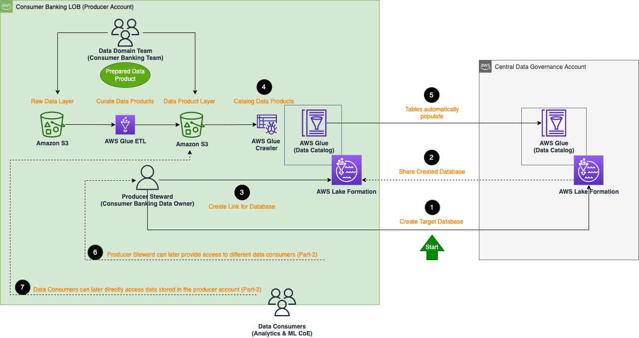
The following diagram illustrates the solution architecture.

The solution workflow consists of the following steps:

When we make a phone call using a landline or cell phone, the Public Switched Telephone Network (PSTN) connects us to the other party. In this demo, we use an Asterisk server (a free contact center framework) deployed on an Amazon EC2 server to emulate a contact center connected to the PSTN through an Amazon Chime Voice Connector. Asterisk is a software implementation of a private branch exchange (PBX)— a controller of a private telephone network used within a company or organization.
As part of this demo, a phone number is acquired via the Amazon Chime SDK and associated with the Asterisk PBX. When a call is made to this number, it’s delivered as SIP (Session Initiation Protocol) to the Asterisk PBX server. The Asterisk PBX then routes this call to the Amazon Chime Voice Connector using SIP, where it triggers an Amazon Chime SIP media application.
Amazon Chime PSTN audio uses a SIP media application to create a programmable VoIP application. The Amazon Chime SIP media application works with a Lambda function to programmatically handle the call.
When the call arrives at the Amazon Chime SIP media application, the associated Lambda function is invoked. The function stores the call information in a DynamoDB table and returns a StartBotConversation action. The StartBotConversation action establishes a voice conversation between the end-user on PSTN and the Amazon Lex bot.
Amazon Lex is a fully managed AWS AI service with advanced natural language models to design, build, test, and deploy conversational interfaces in applications. It combines automatic speech recognition and natural language understanding technologies to create a human-like interaction for your applications. As an example, this demo deploys a bot to perform three automated tasks, or intents: Check Balance, Transfer Funds, and Open Account. An intent represents an action that the user wants to perform.
The conversation starts with the caller interacting with the Amazon Lex bot by telling the bot what they want to do. The automatic speech recognition (ASR) and natural language understanding (NLU) capabilities of the bot help it understand the user input. Amazon Lex is able to determine the intent requested based on the caller input and sample utterances configured for each intent.
After the intent is determined, Amazon Lex interacts with the caller to gather information for all the slots configured for that intent. For example, the Open Account intent includes four slots:
1. First Name
2. Last Name
3. Account Type
4. Phone Number
Amazon Lex works with the caller to capture information for all of these required slots of the selected intent. After these have been captured and the intent has been fulfilled, Amazon Lex returns call processing to the Amazon Chime SIP media application, along with the full results of the Amazon Lex bot conversation.
The subsequent processing steps are performed by the PSTN audio handler Lambda function. This includes parsing the results, determining the next call route action, storing the results in a DynamoDB table, and returning the hang up action.
The Asterisk PBX uses the information stored in the DynamoDB table to determine the next action. For example, if the caller wanted to check their balance, the call ends. However, if the caller wanted to open an account, the call is sent to the agent and includes the information captured in the Amazon Lex bot.

We have used AWS Cloud Development Kit (AWS CDK) to package this application for easy deployment in your account. The AWS CDK is an open-source software development framework to define your cloud application resources using familiar programming languages. It provides high-level components called constructs that preconfigure cloud resources with proven defaults, so you can build cloud applications with ease.

Prerequisites

Before we deploy the solution, we need to have an AWS account and a local machine to run the AWS CDK stack. Complete the following steps:

Log in to your AWS account.
If you don’t have an AWS account, you can sign up for one.For new customers, AWS provides a Free Tier, which provides the ability to explore and try out AWS services free of charge (up to the specified limits for each service). This can help you gain hands-on experience with the AWS platform, products, and services.We use a local machine, such as a laptop or a desktop computer, to deploy the stack using AWS CDK.
Open a new terminal window for MacOS, or putty for Windows OS to install all the prerequisites required to deploy the solution.
Install the following prerequisite software:
1. AWS Command Line Interface (AWS CLI) – A command line tool for interacting with AWS services. For installation instructions, refer to Installing, updating, and uninstalling the AWS CLI.
2. Node.js > 16 – Open-source JavaScript backend engine for application development and deployment. For installation instructions, refer to Tutorial: Setting Up Node.js on an Amazon EC2 Instance.
3. Yarn – Yarn is a package manager for your code. It allows easy access to use and share the code between developers. Run the following command to install Yarn:
```
curl -o- -L https://yarnpkg.com/install.sh | bash
```
  Now we run the following commands to set up the AWS access keys we need. For more information, refer to Managing access keys for IAM users.
Run the following command:
```
aws configure list
```
Run the following command:
```
aws configure
```
Provide the values for your AWS account’s access key ID and secret access key.
Change the Region name or leave the default Region as it is.
Accept the default value of JSON for the output format.

Deploy the solution

You can also customize this solution for your requirements. Review the output resources this deployment contains and modify the Lambda function to add the custom business logic you need for your own solution.

Run the following steps in the same terminal to deploy the application:

Clone the git repository:

git clone https://github.com/aws-samples/amazon-chime-pstn-audio-with-amazon-lex.git

Enter the project directory:

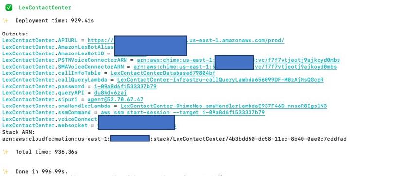
cd amazon-chime-pstn-audio-with-amazon-lex
Deploy the AWS CDK application:
```
yarn launch
```
After a few minutes, your stack deployment should be complete. The following screenshot shows the sample output.
Install the web client SIP phone with the following commands:
```
cd site 
```
```
Yarn 
```
```
yarn run start
```

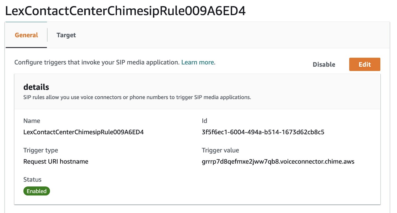
Review the Amazon Chime SDK Voice Connector

In this post, we use the Amazon Chime SDK to route the calls received on the Asterisk PBX server (or your existing contact centers) to Amazon Lex. This is done using Amazon Chime SIP PSTN audio and the Amazon Chime Voice Connector. Amazon Chime PSTN audio enables you to create programmable telephony applications using Lambda functions. These Amazon Chime SIP media applications are triggered by either a PSTN phone number or Amazon Chime Voice Connector. The following screenshot shows the SIP rule that is triggered by an Amazon Chime SDK Voice Connector and targets a SIP media application.

Review the Account Balance chatbot

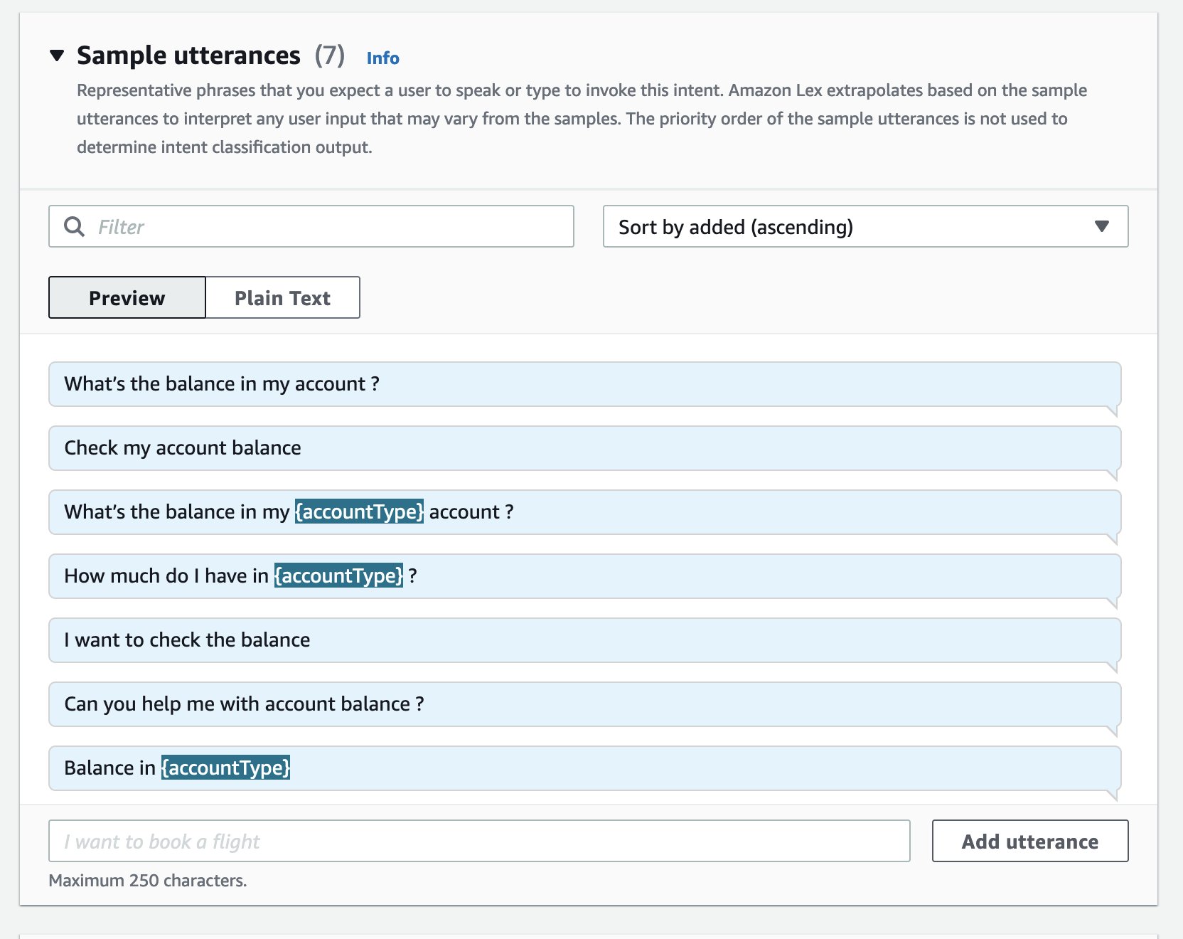
The Amazon Lex bot in this demo includes three intents. These intents can be requested through natural language speech from the caller. For example, the Check Balance intent is seeded with the following sample utterances.

An intent can require zero or more parameters, which are called slots. We add slots as part of the intent configuration while building the blot. At runtime, Amazon Lex prompts the user for specific slot values. The user must provide values for all required slots before Amazon Lex can fulfill the intent.

For the Check Balance intent, Amazon Lex prompts for slot data, such as:

For which account would you like to check the balance?
For verification purposes, what is your date of birth?

After the Amazon Lex bot gathers all the required slot information, it fulfills the intent by invoking the appropriate response. In this case, it queries the account balance related to the account and provides it to the customer.

In this post, we’re using a Lambda function to help initialize, validate, and fulfill the intent. The following is the sample Python code showing how the function handles invocations depending on which intent is being used:

def dispatch(intent_request):
    intent_name = intent_request["sessionState"]["intent"]["name"]
    response = None
    # Dispatch to your bot's intent handlers
    if intent_name == "CheckBalance":
        return CheckBalance(intent_request)
    elif intent_name == "FollowupCheckBalance":
        return FollowupCheckBalance(intent_request)
    elif intent_name == "OpenAccount":
        return OpenAccount(intent_request)

    raise Exception("Intent with name " + intent_name + " not supported")


def lambda_handler(event, context):
    print(event)
    response = dispatch(event)
    print(response)
    return response

The following is the sample code that explains the code block for the Check Balance intent in the Lambda function. In this example, we generate a random number as the account balance, but this could be integrated with your existing database to provide accurate caller information.

def CheckBalance(intent_request):
    session_attributes = get_session_attributes(intent_request)
    slots = get_slots(intent_request)
    account = get_slot(intent_request, "accountType")
    # The account balance in this case is a random number
    # Here is where you could query a system to get this information
    balance = str(random_num())
    text = "Thank you. The balance on your " + account + " account is $" + balance
    message = {"contentType": "PlainText", "content": text}
    fulfillment_state = "Fulfilled"
    return close(session_attributes, "CheckBalance", fulfillment_state, message)

Test the solution

Let’s walk through the solution by following the path of a single user request:

Get the phone number from the output after deploying the AWS CDK:
```
Outputs:
LexContactCenter.voiceConnectorPhone = +1NPANXXXXXX
```
Dial into the phone number from any PSTN-based phone.
Now you can try the menu options.

For the Amazon Lex bot to understand the Check Balance intent, you can speak any of the following utterances:

What’s the balance in my account?
Check my account balance?
I want to check the balance?

Amazon Lex prompts for the slot data that’s required to fulfill this intent. For the Check Balance intent, Amazon Lex prompts for the account and date of birth:

For which account would you like to check the balance?
For verification purposes, what is your data of birth?

After you provide the required information, the bot fulfills the intent and provides the account balance information. The following is a sample output message for the Check Balance intent: Thank you. The balance on your <account> account is $<balance>.

Complete the call by hanging up or being transferred to an agent.

When the conversation with the Amazon Lex bot is complete, the call returns to the SIP media application and associated Lambda function with the results from the bot conversation.

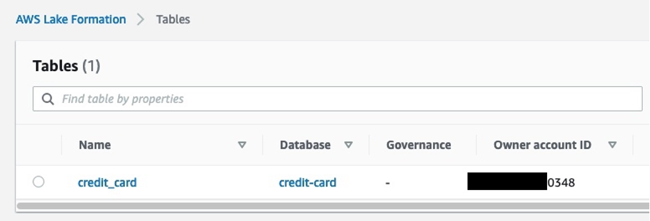
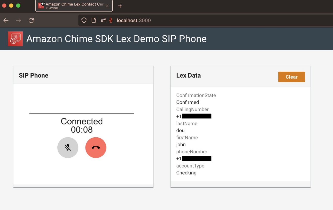
The Amazon Chime SIP media application performs the post-processing steps and returns the call to the Asterisk PBX. For the Open Account intent, this causes the Asterisk PBX to call an agent using a web client-based SIP phone. The following screenshot shows the dashboard with the agent call information. This call can be answered on the web client to establish two-way audio between the caller and the agent. As shown in the screenshot, the information provided by the caller has been preserved and presented to the agent.

Watch the following video for an example of a partner solution on how to integrate Amazon Lex with Cisco Unified Contact Center using Amazon Chime SDK:

Clean up resources

To clean up the resources used in this demo and avoid incurring further charges, run the following command in the terminal window:

yarn destroy

The AWS CloudFormation stack created by the AWS CDK is destroyed, removing all the allocated resources.

Conclusion

In this post, we demonstrated a solution with a reference architecture to add self-service AI to any contact center using Amazon Lex and the Amazon Chime SDK. We showed how the solution works and provided a detailed walkthrough of the code and deployment steps. This solution is meant to be a reference architecture or a quick start guide that you can customize for your own needs.

Give it a whirl and let us know how this solved your use case by leaving feedback in the comments section. For more information, see the project GitHub repository.

About the authors

Prem Ranga is a NLP domain lead and a Sr. AI/ML specialist SA at AWS and an author who frequently publishes blogs, research papers, and recently a NLP text book. When he is not helping customers adopt AWS AI/ML, Prem dabbles with building Simple Beer Service units for AWS offices, running competitive gaming events with DeepRacer & DeepComposer, and educating students, young professionals on career building AI/ML skills. You can follow Prem’s work on LinkedIn.

Court Schuett is the Lead Evangelist for the Amazon Chime SDK with a background in telephony and now loves to build things that build things. Court is focused on teaching developers and non-developers alike how to build with AWS.

Vamshi Krishna Enabothala is a Senior AI/ML Specialist SA at AWS with expertise in big data, analytics, and orchestrating scalable AI/ML architectures for startups and enterprises. Vamshi is focused on Language AI and innovates in building world-class recommender engines. Outside of work, Vamshi is an RC enthusiast, building and playing with RC equipment (planes, cars, and drones), and also enjoys gardening.

Identify the location of anomalies using Amazon Lookout for Vision at the edge without using a GPU

Automated defect detection using computer vision helps improve quality and lower the cost of inspection. Defect detection involves identifying the presence of a defect, classifying types of defects, and identifying where the defects are located. Many manufacturing processes require detection at a low latency, with limited compute resources, and with limited connectivity.

Amazon Lookout for Vision is a machine learning (ML) service that helps spot product defects using computer vision to automate the quality inspection process in your manufacturing lines, with no ML expertise required. Lookout for Vision now includes the ability to provide the location and type of anomalies using semantic segmentation ML models. These customized ML models can either be deployed to the AWS Cloud using cloud APIs or to custom edge hardware using AWS IoT Greengrass. Lookout for Vision now supports inference on an x86 compute platform running Linux with or without an NVIDIA GPU accelerator and on any NVIDIA Jetson-based edge appliance. This flexibility allows detection of defects on existing or new hardware.

In this post, we show you how to detect defective parts using Lookout for Vision ML models running on an edge appliance, which we simulate using an Amazon Elastic Compute Cloud (Amazon EC2) instance. We walk through training the new semantic segmentation models, exporting them as AWS IoT Greengrass components, and running inference in CPU-only mode with Python example code.

Solution overview

In this post, we use a set of pictures of toy aliens composed of normal and defective images such as missing limbs, eyes, or other parts. We train a Lookout for Vision model in the cloud to identify defective toy aliens. We compile the model to a target X86 CPU, package the trained Lookout for Vision model as an AWS IoT Greengrass component, and deploy the model to an EC2 instance without a GPU using the AWS IoT Greengrass console. Finally, we demonstrate a Python-based sample application running on the EC2 (C5a.2xl) instance that sources the toy alien images from the edge device file system, runs the inference on the Lookout for Vision model using the gRPC interface, and sends the inference data to an MQTT topic in the AWS Cloud. The scripts outputs an image that includes the color and location of the defects on the anomalous image.

The following diagram illustrates the solution architecture. It’s important to note for each defect type you want to detect in localization, you must have 10 marked anomaly images in training and 10 in test data, for a total of 20 images of that type. For this post, we search for missing limbs on the toy.

The solution has the following workflow:

Upload a training dataset and a test dataset to Amazon Simple Storage Service (Amazon S3).
Use the new Lookout for Vision UI to add an anomaly type and mark where those anomalies are in the training and test images.
Train a Lookout for Vision model in the cloud.
Compile the model to the target architecture (X86) and deploy the model to the EC2 (C5a.2xl) instance using the AWS IoT Greengrass console.
Source images from local disk.
Run inferences on the deployed model via the gRPC interface and retrieve an image of anomaly masks overlaid on the original image.
Post the inference results to an MQTT client running on the edge instance.
Receive the MQTT message on a topic in AWS IoT Core in the AWS Cloud for further monitoring and visualization.

Steps 5, 6, and 7 are coordinated with the sample Python application.

Prerequisites

Before you get started, complete the following prerequisites. For this post, we use an EC2 c5.2xl instance and install AWS IoT Greengrass V2 on it to try out the new features. If you want to run on an NVIDIA Jetson, follow the steps in our previous post, Amazon Lookout for Vision now supports visual inspection of product defects at the edge.

Create an AWS account.
Start an EC2 instance that we can install AWS IoT Greengrass on and use the new CPU-only inference mode.You can also use an Intel X86 64 bit machine with 8 gigabytes of ram or more (we use a c5a.2xl, but anything with greater than 8 gigabytes on x86 platform should work) running Ubuntu 20.04.

Install AWS IoT Greengrass V2:

git clone https://github.com/aws-samples/amazon-lookout-for-vision.git
cd edge
# be sure to edit the installation script to match your region, also adjust any device names and groups!
vi install_greengrass.sh

Install the needed system and Python 3 dependencies (Ubuntu 20.04):

# install Ubuntu dependencies on the EC2 instance
./install-ec2-ubuntu-deps.sh
pip3 install -r requirements.txt
# Replace ENDPOINT variable in sample-client-file-mqtt.py with the value on the AWS console AWS IoT->Things->l4JetsonXavierNX->Interact.  
# Under HTTPS. It will be of type <name>-ats.iot.<region>.amazon.com

Upload the dataset and train the model

We use the toy aliens dataset to demonstrate the solution. The dataset contains normal and anomalous images. Here are a few sample images from the dataset.

The following image shows a normal toy alien.

The following image shows a toy alien missing a leg.

The following image shows a toy alien missing a head.

In this post, we look for missing limbs. We use the new user interface to draw a mask around the defects in our training and tests data. This will tell the semantic segmentation models how to identify this type of defect.

Start by uploading your dataset, either via Amazon S3 or from your computer.
Sort them into folders titled normal and anomaly.
When creating your dataset, select Automatically attach labels to images based on the folder name.This allows us to sort out the anomalous images later and draw in the areas to be labeled with a defect.
Try to hold back some images for testing later of both normal and anomaly.
After all the images have been added to the dataset, choose Add anomaly labels.
Begin labeling data by choosing Start labeling.
To speed up the process, you can select multiple images and classify them as Normal or Anomaly.

If you want to highlight anomalies in addition to classifying them, you need to highlight where the anomalies are located.
Choose the image you want to annotate.
Use the drawing tools to show the area where part of the subject is missing, or draw a mask over the defect.
Choose Submit and close to keep these changes.
Repeat this process for all your images.
When you’re done, choose Save to persist your changes. Now you’re ready to train your model.
Choose Train model.

After you complete these steps, you can navigate to the project and the Models page to check the performance of the trained model. You can start the process of exporting the model to the target edge device any time after the model is trained.

Retrain the model with corrected images

Sometimes the anomaly tagging may not be quite correct. You have the chance to help your model learn your anomalies better. For example, the following image is identified as an anomaly, but doesn’t show the missing_limbs tag.

Let’s open the editor and fix this.

Go through any images you find like this. If you find it’s tagged an anomaly incorrectly, you can use the eraser tool to remove the incorrect tag.

You can now train your model again and achieve better accuracy.

Compile and package the model as an AWS IoT Greengrass component

In this section, we walk through the steps to compile the toy alien model to our target edge device and package the model as an AWS IoT Greengrass component.

On the Lookout for Vision console, choose your project.
In the navigation pane, choose Edge model packages.
Choose Create model packaging job.
For Job name, enter a name.
For Job description, enter an optional description.
Choose Browse models.
Select the model version (the toy alien model built in the previous section).
Choose Choose.
If you’re running this on Amazon EC2 or an X86-64 device, select Target platform and choose Linux, X86, and CPU.
If using CPU, you can leave the compiler options empty if you’re not sure and don’t have an NVIDIA GPU. If you have an Intel-based platform that supports AVX512, you can add these compiler options to optimize for better performance: {"mcpu": "skylake-avx512"}.
You can see your job name and status showing as In progress. The model packaging job may take a few minutes to complete.When the model packaging job is complete, the status shows as Success.
Choose your job name (in our case it’s aliensblogcpux86) to see the job details.
Choose Create model packaging job.
Enter the details for Component name, Component description (optional), Component version, and Component location.Lookout for Vision stores the component recipes and artifacts in this Amazon S3 location.
Choose Continue deployment in Greengrass to deploy the component to the target edge device.

The AWS IoT Greengrass component and model artifacts have been created in your AWS account.

Deploy the model

Be sure you have AWS IoT Greengrass V2 installed on your target device for your account before you continue. For instructions, refer to Install the AWS IoT Greengrass Core software.

In this section, we walk through the steps to deploy the toy alien model to the edge device using the AWS IoT Greengrass console.

On the AWS IoT Greengrass console, navigate to your edge device.
Choose Deploy to initiate the deployment steps.
Select Core device (because the deployment is to a single device) and enter a name for Target name.The target name is the same name you used to name the core device during the AWS IoT Greengrass V2 installation process.
Choose your component. In our case, the component name is aliensblogcpux86, which contains the toy alien model.
Choose Next.
Configure the component (optional).
Choose Next.
Expand Deployment policies.
For Component update policy, select Notify components.This allows the already deployed component (a prior version of the component) to defer an update until you’re ready to update.
For Failure handling policy, select Don’t roll back.In case of a failure, this option allows us to investigate the errors in deployment.
Choose Next.
Review the list of components that will be deployed on the target (edge) device.
Choose Next.You should see the message Deployment successfully created.
To validate the model deployment was successful, run the following command on your edge device:
```
sudo /greengrass/v2/bin/greengrass-cli component list
```

You should see a similar output running the aliensblogcpux86 lifecycle startup script:

Components currently running in Greengrass:

Components currently running in Greengrass:
 
Component Name: aws.iot.lookoutvision.EdgeAgent
    Version: 0.1.34
    State: RUNNING
    Configuration: {"Socket":"unix:///tmp/aws.iot.lookoutvision.EdgeAgent.sock"}
 Component Name: aliensblogcpux86
    Version: 1.0.0
    State: RUNNING
    Configuration: {"Autostart":false}

Run inferences on the model

Note: If you are running Greengrass as another user than what you are logged in as, you will need to change permissions of the file /tmp/aws.iot.lookoutvision.EdgeAgent.sock:

chmod 666 /tmp/aws.iot.lookoutvision.EdgeAgent.sock

We’re now ready to run inferences on the model. On your edge device, run the following command to load the model (replace <modelName> with the model name used in your component):

# run command to load the model# This will load the model into running state pass
# the name of the model component as a parameter.
python3 warmup-model.py <modelName>

To generate inferences, run the following command with the source file name (replace <path/to/images> with the path and file name of the image to check and replace <modelName> with the model name used for your component):

python3 sample-client-file-mqtt.py </path/to/images> <modelName>

start client ['sample-client-file.py', 'aliens-dataset/anomaly/1.png', 'aliensblogcpux86']
channel set
shape=(380, 550, 3)
Image is anomalous, (90.05860090255737 % confidence) contains defects with total area over .1%: {'missing_limbs': '#FFFFFF'}

The model correctly predicts the image as anomalous (missing_limbs) with a confidence score of 0.9996867775917053. It tells us the mask of the anomaly tag missing_limbs and the percentage area. The response also contains bitmap data you can decode of what it found.

Download and open the file blended.png, which looks like the following image. Note the area highlighted with the defect around the legs.

Customer stories

With AWS IoT Greengrass and Lookout for Vision, you can now automate visual inspection with computer vision for processes like quality control and defect assessment—all on the edge and in real time. You can proactively identify problems such as parts damage (like dents, scratches, or poor welding), missing product components, or defects with repeating patterns on the production line itself—saving you time and money. Customers like Tyson and Baxter are discovering the power of Lookout for Vision to increase quality and reduce operational costs by automating visual inspection.

“Operational excellence is a key priority at Tyson Foods. Predictive maintenance is an essential asset for achieving this objective by continuously improving overall equipment effectiveness (OEE). In 2021, Tyson Foods launched a machine learning-based computer vision project to identify failing product carriers during production to prevent them from impacting team member safety, operations, or product quality. The models trained using Amazon Lookout for Vision performed well. The pin detection model achieved 95% accuracy across both classes. The Amazon Lookout for Vision model was tuned to perform at 99.1% accuracy for failing pin detection. By far the most exciting result of this project was the speedup in development time. Although this project utilizes two models and a more complex application code, it took 12% less developer time to complete. This project for monitoring the condition of the product carriers at Tyson Foods was completed in record time using AWS managed services such as Amazon Lookout for Vision.”

—Audrey Timmerman, Sr Applications Developer, Tyson Foods.

“Latency and inferencing speed is critical for real-time assessment and critical quality checks of our manufacturing processes. Amazon Lookout for Vision edge on a CPU device gives us the ability to achieve this on production-grade equipment, enabling us to deliver cost-effective AI vision solutions at scale.”

—A.K. Karan, Global Senior Director – Digital Transformation, Integrated Supply Chain, Baxter International Inc.

Cleanup

Complete the following steps to remove the assets you created from your account and avoid any ongoing billing:

On the Lookout for Vision console, navigate to your project.
On the Actions menu, delete your datasets.
Delete your models.
On the Amazon S3 console, empty the buckets you created, then delete the buckets.
On the Amazon EC2 console, delete the instance you started to run AWS IoT Greengrass.
On the AWS IoT Greengrass console, choose Deployments in the navigation pane.
Delete your component versions.
On the AWS IoT Greengrass console, delete the AWS IoT things, groups, and devices.

Conclusion

In this post, we described a typical scenario for industrial defect detection at the edge using defect localization and deployed to a CPU-only device. We walked through the key components of the cloud and edge lifecycle with an end-to-end example using Lookout for Vision and AWS IoT Greengrass. With Lookout for Vision, we trained an anomaly detection model in the cloud using the toy alien dataset, compiled the model to a target architecture, and packaged the model as an AWS IoT Greengrass component. With AWS IoT Greengrass, we deployed the model to an edge device. We demonstrated a Python-based sample application that sources toy alien images from the edge device local file system, runs the inferences on the Lookout for Vision model at the edge using the gRPC interface, and sends the inference data to an MQTT topic in the AWS Cloud.

In a future post, we will show how to run inferences on a real-time stream of images using a GStreamer media pipeline.

Start your journey towards industrial anomaly detection and identification by visiting the Amazon Lookout for Vision and AWS IoT Greengrass resource pages.

About the authors

Manish Talreja is a Senior Industrial ML Practice Manager with AWS Professional Services. He helps AWS customers achieve their business goals by architecting and building innovative solutions that use AWS ML and IoT services on the AWS Cloud.

Ryan Vanderwerf is a partner solutions architect at Amazon Web Services. He previously provided Java virtual machine-focused consulting and project development as a software engineer at OCI on the Grails and Micronaut team. He was chief architect/director of products at ReachForce, with a focus on software and system architecture for AWS Cloud SaaS solutions for marketing data management. Ryan has built several SaaS solutions in several domains such as financial, media, telecom, and e-learning companies since 1996.

Prakash Krishnan is a Senior Software Development Manager at Amazon Web Services. He leads the engineering teams that are building large-scale distributed systems to apply fast, efficient, and highly scalable algorithms to deep learning-based image and video recognition problems.

Fine-tune and deploy a summarizer model using the Hugging Face Amazon SageMaker containers bringing your own script

There have been many recent advancements in the NLP domain. Pre-trained models and fully managed NLP services have democratised access and adoption of NLP. Amazon Comprehend is a fully managed service that can perform NLP tasks like custom entity recognition, topic modelling, sentiment analysis and more to extract insights from data without the need of any prior ML experience.

Last year, AWS announced a partnership with Hugging Face to help bring natural language processing (NLP) models to production faster. Hugging Face is an open-source AI community, focused on NLP. Their Python-based library (Transformers) provides tools to easily use popular state-of-the-art Transformer architectures like BERT, RoBERTa, and GPT. You can apply these models to a variety of NLP tasks, such as text classification, information extraction, and question answering, among others.

Amazon SageMaker is a fully managed service that provides developers and data scientists the ability to build, train, and deploy machine learning (ML) models quickly. SageMaker removes the heavy lifting from each step of the ML process, making it easier to develop high-quality models. The SageMaker Python SDK provides open-source APIs and containers to train and deploy models on SageMaker, using several different ML and deep learning frameworks.

The Hugging Face integration with SageMaker allows you to build Hugging Face models at scale on your own domain-specific use cases.

In this post, we walk you through an example of how to build and deploy a custom Hugging Face text summarizer on SageMaker. We use Pegasus [1] for this purpose, the first Transformer-based model specifically pre-trained on an objective tailored for abstractive text summarization. BERT is pre-trained on masking random words in a sentence; in contrast, during Pegasus’s pre-training, sentences are masked from an input document. The model then generates the missing sentences as a single output sequence using all the unmasked sentences as context, creating an executive summary of the document as a result.

Thanks to the flexibility of the HuggingFace library, you can easily adapt the code shown in this post for other types of transformer models, such as t5, BART, and more.

Load your own dataset to fine-tune a Hugging Face model

To load a custom dataset from a CSV file, we use the load_dataset method from the Transformers package. We can apply tokenization to the loaded dataset using the datasets.Dataset.map function. The map function iterates over the loaded dataset and applies the tokenize function to each example. The tokenized dataset can then be passed to the trainer for fine-tuning the model. See the following code:

# Python
def tokenize(batch):
    tokenized_input = tokenizer(batch[args.input_column], padding='max_length', truncation=True, max_length=args.max_source)
    tokenized_target = tokenizer(batch[args.target_column], padding='max_length', truncation=True, max_length=args.max_target)
    tokenized_input['target'] = tokenized_target['input_ids']

    return tokenized_input
    

def load_and_tokenize_dataset(data_dir):
    for file in os.listdir(data_dir):
        dataset = load_dataset("csv", data_files=os.path.join(data_dir, file), split='train')
    tokenized_dataset = dataset.map(lambda batch: tokenize(batch), batched=True, batch_size=512)
    tokenized_dataset.set_format('numpy', columns=['input_ids', 'attention_mask', 'labels'])
    
    return tokenized_dataset

Build your training script for the Hugging Face SageMaker estimator

As explained in the post AWS and Hugging Face collaborate to simplify and accelerate adoption of Natural Language Processing models, training a Hugging Face model on SageMaker has never been easier. We can do so by using the Hugging Face estimator from the SageMaker SDK.

The following code snippet fine-tunes Pegasus on our dataset. You can also find many sample notebooks that guide you through fine-tuning different types of models, available directly in the transformers GitHub repository. To enable distributed training, we can use the Data Parallelism Library in SageMaker, which has been built into the HuggingFace Trainer API. To enable data parallelism, we need to define the distribution parameter in our Hugging Face estimator.

# Python
from sagemaker.huggingface import HuggingFace
# configuration for running training on smdistributed Data Parallel
distribution = {'smdistributed':{'dataparallel':{ 'enabled': True }}}
huggingface_estimator = HuggingFace(entry_point='train.py',
                                    source_dir='code',
                                    base_job_name='huggingface-pegasus',
                                    instance_type= 'ml.g4dn.16xlarge',
                                    instance_count=1,
                                    transformers_version='4.6',
                                    pytorch_version='1.7',
                                    py_version='py36',
                                    output_path=output_path,
                                    role=role,
                                    hyperparameters = {
                                        'model_name': 'google/pegasus-xsum',
                                        'epoch': 10,
                                        'per_device_train_batch_size': 2
                                    },
                                    distribution=distribution)
huggingface_estimator.fit({'train': training_input_path, 'validation': validation_input_path, 'test': test_input_path})

The maximum training batch size you can configure depends on the model size and the GPU memory of the instance used. If SageMaker distributed training is enabled, the total batch size is the sum of every batch that is distributed across each device/GPU. If we use an ml.g4dn.16xlarge with distributed training instead of an ml.g4dn.xlarge instance, we have eight times (8 GPUs) as much memory as a ml.g4dn.xlarge instance (1 GPU). The batch size per device remains the same, but eight devices are training in parallel.

As usual with SageMaker, we create a train.py script to use with Script Mode and pass hyperparameters for training. The following code snippet for Pegasus loads the model and trains it using the Transformers Trainer class:

# Python
from transformers import (
    AutoModelForSeq2SeqLM,
    AutoTokenizer,
    Seq2SeqTrainer,
    Seq2seqTrainingArguments
)

model = AutoModelForSeq2SeqLM.from_pretrained(model_name).to(device)
    
training_args = Seq2seqTrainingArguments(
    output_dir=args.model_dir,
    num_train_epochs=args.epoch,
    per_device_train_batch_size=args.train_batch_size,
    per_device_eval_batch_size=args.eval_batch_size,
    warmup_steps=args.warmup_steps,
    weight_decay=args.weight_decay,
    logging_dir=f"{args.output_data_dir}/logs",
    logging_strategy='epoch',
    evaluation_strategy='epoch',
    saving_strategy='epoch',
    adafactor=True,
    do_train=True,
    do_eval=True,
    do_predict=True,
    save_total_limit = 3,
    load_best_model_at_end=True,
    metric_for_best_model='eval_loss'
    # With the goal to deploy the best checkpoint to production
    # it is important to set load_best_model_at_end=True,
    # this makes sure that the last model is saved at the root
    # of the model_dir” directory
)
    
trainer = Seq2SeqTrainer(
    model=model,
    args=training_args,
    train_dataset=dataset['train'],
    eval_dataset=dataset['validation']
)

trainer.train()
trainer.save_model()

# Get rid of unused checkpoints inside the container to limit the model.tar.gz size
os.system(f"rm -rf {args.model_dir}/checkpoint-*/")

The full code is available on GitHub.

Deploy the trained Hugging Face model to SageMaker

Our friends at Hugging Face have made inference on SageMaker for Transformers models simpler than ever thanks to the SageMaker Hugging Face Inference Toolkit. You can directly deploy the previously trained model by simply setting up the environment variable "HF_TASK":"summarization" (for instructions, see Pegasus Models), choosing Deploy, and then choosing Amazon SageMaker, without needing to write an inference script.

However, if you need some specific way to generate or postprocess predictions, for example generating several summary suggestions based on a list of different text generation parameters, writing your own inference script can be useful and relatively straightforward:

# Python
# inference.py script

import os
import json
import torch
from transformers import AutoModelForSeq2SeqLM, AutoTokenizer

device = torch.device("cuda" if torch.cuda.is_available() else "cpu")

def model_fn(model_dir):
    # Create the model and tokenizer and load weights
    # from the previous training Job, passed here through "model_dir"
    # that is reflected in HuggingFaceModel "model_data"
    tokenizer = AutoTokenizer.from_pretrained(model_dir)
    model = AutoModelForSeq2SeqLM.from_pretrained(model_dir).to(device).eval()
    
    model_dict = {'model':model, 'tokenizer':tokenizer}
    
    return model_dict
        

def predict_fn(input_data, model_dict):
    # Return predictions/generated summaries
    # using the loaded model and tokenizer on input_data
    text = input_data.pop('inputs')
    parameters_list = input_data.pop('parameters_list', None)
    
    tokenizer = model_dict['tokenizer']
    model = model_dict['model']

    # Parameters may or may not be passed    
    input_ids = tokenizer(text, truncation=True, padding='longest', return_tensors="pt").input_ids.to(device)
    
    if parameters_list:
        predictions = []
        for parameters in parameters_list:
            output = model.generate(input_ids, **parameters)
            predictions.append(tokenizer.batch_decode(output, skip_special_tokens=True))
    else:
        output = model.generate(input_ids)
        predictions = tokenizer.batch_decode(output, skip_special_tokens=True)
    
    return predictions
    
    
def input_fn(request_body, request_content_type):
    # Transform the input request to a dictionary
    request = json.loads(request_body)
    return request

As shown in the preceding code, such an inference script for HuggingFace on SageMaker only needs the following template functions:

model_fn() – Reads the content of what was saved at the end of the training job inside SM_MODEL_DIR, or from an existing model weights directory saved as a tar.gz file in Amazon Simple Storage Service (Amazon S3). It’s used to load the trained model and associated tokenizer.
input_fn() – Formats the data received from a request made to the endpoint.
predict_fn() – Calls the output of model_fn() (the model and tokenizer) to run inference on the output of input_fn() (the formatted data).

Optionally, you can create an output_fn() function for inference formatting, using the output of predict_fn(), which we didn’t demonstrate in this post.

We can then deploy the trained Hugging Face model with its associated inference script to SageMaker using the Hugging Face SageMaker Model class:

# Python
from sagemaker.huggingface import HuggingFaceModel

model = HuggingFaceModel(model_data=huggingface_estimator.model_data,
                     role=role,
                     framework_version='1.7',
                     py_version='py36',
                     entry_point='inference.py',
                     source_dir='code')
                     
predictor = model.deploy(initial_instance_count=1,
                         instance_type='ml.g4dn.xlarge'
                         )

Test the deployed model

For this demo, we trained the model on the Women’s E-Commerce Clothing Reviews dataset, which contains reviews of clothing articles (which we consider as the input text) and their associated titles (which we consider as summaries). After we remove articles with missing titles, the dataset contains 19,675 reviews. Fine-tuning the Pegasus model on a training set containing 70% of those articles for five epochs took approximately 3.5 hours on an ml.p3.16xlarge instance.

We can then deploy the model and test it with some example data from the test set. The following is an example review describing a sweater:

# Python
Review Text
"I ordered this sweater in green in petite large. The color and knit is beautiful and the shoulders and body fit comfortably; however, the sleeves were very long for a petite. I roll them, and it looks okay but would have rather had a normal petite length sleeve."

Original Title
"Long sleeves"

Rating
3

Thanks to our custom inference script hosted in a SageMaker endpoint, we can generate several summaries for this review with different text generation parameters. For example, we can ask the endpoint to generate a range of very short to moderately long summaries specifying different length penalties (the smaller the length penalty, the shorter the generated summary). The following are some parameter input examples, and the subsequent machine-generated summaries:

# Python
inputs = {
    "inputs":[
"I ordered this sweater in green in petite large. The color and knit is   beautiful and the shoulders and body fit comfortably; however, the sleeves were very long for a petite. I roll them, and it looks okay but would have rather had a normal petite length sleeve."
    ],

    "parameters_list":[
        {
            "length_penalty":2
        },
	{
            "length_penalty":1
        },
	{
            "length_penalty":0.6
        },
        {
            "length_penalty":0.4
        }
    ]

result = predictor.predict(inputs)
print(result)

[
    ["Beautiful color and knit but sleeves are very long for a petite"],
    ["Beautiful sweater, but sleeves are too long for a petite"],
    ["Cute, but sleeves are long"],
    ["Very long sleeves"]
]

Which summary do you prefer? The first generated title captures all the important facts about the review, with a quarter the number of words. In contrast, the last one only uses three words (less than 1/10th the length of the original review) to focus on the most important feature of the sweater.

Conclusion

You can fine-tune a text summarizer on your custom dataset and deploy it to production on SageMaker with this simple example available on GitHub. Additional sample notebooks to train and deploy Hugging Face models on SageMaker are also available.

As always, AWS welcomes feedback. Please submit any comments or questions.

References

[1] PEGASUS: Pre-training with Extracted Gap-sentences for Abstractive Summarization

About the authors

Viktor Malesevic is a Machine Learning Engineer with AWS Professional Services, passionate about Natural Language Processing and MLOps. He works with customers to develop and put challenging deep learning models to production on AWS. In his spare time, he enjoys sharing a glass of red wine and some cheese with friends.

Aamna Najmi is a Data Scientist with AWS Professional Services. She is passionate about helping customers innovate with Big Data and Artificial Intelligence technologies to tap business value and insights from data. In her spare time, she enjoys gardening and traveling to new places.

Team and user management with Amazon SageMaker and AWS SSO

Amazon SageMaker Studio is a web-based integrated development environment (IDE) for machine learning (ML) that lets you build, train, debug, deploy, and monitor your ML models. Each onboarded user in Studio has their own dedicated set of resources, such as compute instances, a home directory on an Amazon Elastic File System (Amazon EFS) volume, and a dedicated AWS Identity and Access Management (IAM) execution role.

One of the most common real-world challenges in setting up user access for Studio is how to manage multiple users, groups, and data science teams for data access and resource isolation.

Many customers implement user management using federated identities with AWS Single Sign-On (AWS SSO) and an external identity provider (IdP), such as Active Directory (AD) or AWS Managed Microsoft AD directory. It’s aligned with the AWS recommended practice of using temporary credentials to access AWS accounts.

An Amazon SageMaker domain supports AWS SSO and can be configured in AWS SSO authentication mode. In this case, each entitled AWS SSO user has their own Studio user profile. Users given access to Studio have a unique sign-in URL that directly opens Studio, and they sign in with their AWS SSO credentials. Organizations manage their users in AWS SSO instead of the SageMaker domain. You can assign multiple users access to the domain at the same time. You can use Studio user profiles for each user to define their security permissions in Studio notebooks via an IAM role attached to the user profile, called an execution role. This role controls permissions for SageMaker operations according to its IAM permission policies.

In AWS SSO authentication mode, there is always one-to-one mapping between users and user profiles. The SageMaker domain manages the creation of user profiles based on the AWS SSO user ID. You can’t create user profiles via the AWS Management Console. This works well in the case when one user is a member of only one data science team or if users have the same or very similar access requirements across their projects and teams. In a more common use case, when a user can participate in multiple ML projects and be a member of multiple teams with slightly different permission requirements, the user requires access to different Studio user profiles with different execution roles and permission policies. Because you can’t manage user profiles independently of AWS SSO in AWS SSO authentication mode, you can’t implement a one-to-many mapping between users and Studio user profiles.

If you need to establish a strong separation of security contexts, for example for different data categories, or need to entirely prevent the visibility of one group of users’ activity and resources to another, the recommended approach is to create multiple SageMaker domains. At the time of this writing, you can create only one domain per AWS account per Region. To implement the strong separation, you can use multiple AWS accounts with one domain per account as a workaround.

The second challenge is to restrict access to the Studio IDE to only users from inside a corporate network or a designated VPC. You can achieve this by using IAM-based access control policies. In this case, the SageMaker domain must be configured with IAM authentication mode, because the IAM identity-based polices aren’t supported by the sign-in mechanism in AWS SSO mode. The post Secure access to Amazon SageMaker Studio with AWS SSO and a SAML application solves this challenge and demonstrates how to control network access to a SageMaker domain.

This solution addresses these challenges of AWS SSO user management for Studio for a common use case of multiple user groups and a many-to-many mapping between users and teams. The solution outlines how to use a custom SAML 2.0 application as the mechanism to trigger the user authentication for Studio and support multiple Studio user profiles per one AWS SSO user.

You can use this approach to implement a custom user portal with applications backed by the SAML 2.0 authorization process. Your custom user portal can have maximum flexibility on how to manage and display user applications. For example, the user portal can show some ML project metadata to facilitate identifying an application to access.

You can find the solution’s source code in our GitHub repository.

Solution overview

The solution implements the following architecture.

The main high-level architecture components are as follows:

Identity provider – Users and groups are managed in an external identity source, for example in Azure AD. User assignments to AD groups define what permissions a particular user has and which Studio team they have access to. The identity source must by synchronized with AWS SSO.
AWS SSO – AWS SSO manages SSO users, SSO permission sets, and applications. This solution uses a custom SAML 2.0 application to provide access to Studio for entitled AWS SSO users. The solution also uses SAML attribute mapping to populate the SAML assertion with specific access-relevant data, such as user ID and user team. Because the solution creates a SAML API, you can use any IdP supporting SAML assertions to create this architecture. For example, you can use Okta or even your own web application that provides a landing page with a user portal and applications. For this post, we use AWS SSO.
Custom SAML 2.0 applications – The solution creates one application per Studio team and assigns one or multiple applications to a user or a user group based on entitlements. Users can access these applications from within their AWS SSO user portal based on assigned permissions. Each application is configured with the Amazon API Gateway endpoint URL as its SAML backend.
SageMaker domain – The solution provisions a SageMaker domain in an AWS account and creates a dedicated user profile for each combination of AWS SSO user and Studio team the user is assigned to. The domain must be configured in IAM authentication mode.
Studio user profiles – The solution automatically creates a dedicated user profile for each user-team combination. For example, if a user is a member of two Studio teams and has corresponding permissions, the solution provisions two separate user profiles for this user. Each profile always belongs to one and only one user. Because you have a Studio user profile for each possible combination of a user and a team, you must consider your account limits for user profiles before implementing this approach. For example, if your limit is 500 user profiles, and each user is a member of two teams, you consume that limit 2.5 times faster, and as a result you can onboard 250 users. With a high number of users, we recommend implementing multiple domains and accounts for security context separation. To demonstrate the proof of concept, we use two users, User 1 and User 2, and two Studio teams, Team 1 and Team 2. User 1 belongs to both teams, whereas User 2 belongs to Team 2 only. User 1 can access Studio environments for both teams, whereas User 2 can access only the Studio environment for Team 2.
Studio execution roles – Each Studio user profile uses a dedicated execution role with permission polices with the required level of access for the specific team the user belongs to. Studio execution roles implement an effective permission isolation between individual users and their team roles. You manage data and resource access for each role and not at an individual user level.

The solution also implements an attribute-based access control (ABAC) using SAML 2.0 attributes, tags on Studio user profiles, and tags on SageMaker execution roles.

In this particular configuration, we assume that AWS SSO users don’t have permissions to sign in to the AWS account and don’t have corresponding AWS SSO-controlled IAM roles in the account. Each user signs in to their Studio environment via a presigned URL from an AWS SSO portal without the need to go to the console in their AWS account. In a real-world environment, you might need to set up AWS SSO permission sets for users to allow the authorized users to assume an IAM role and to sign in to an AWS account. For example, you can provide data scientist role permissions for a user to be able to interact with account resources and have the level of access they need to fulfill their role.

Solution architecture and workflow

The following diagram presents the end-to-end sign-in flow for an AWS SSO user.

An AWS SSO user chooses a corresponding Studio application in their AWS SSO portal. AWS SSO prepares a SAML assertion (1) with configured SAML attribute mappings. A custom SAML application is configured with the API Gateway endpoint URL as its Assertion Consumer Service (ACS), and needs mapping attributes containing the AWS SSO user ID and team ID. We use ssouserid and teamid custom attributes to send all needed information to the SAML backend.

The API Gateway calls an SAML backend API. An AWS Lambda function (2) implements the API, parses the SAML response to extract the user ID and team ID. The function uses them to retrieve a team-specific configuration, such as an execution role and SageMaker domain ID. The function checks if a required user profile exists in the domain, and creates a new one with the corresponding configuration settings if no profile exists. Afterwards, the function generates a Studio presigned URL for a specific Studio user profile by calling CreatePresignedDomainUrl API (3) via a SageMaker API VPC endpoint. The Lambda function finally returns the presigned URL with HTTP 302 redirection response to sign the user in to Studio.

The solution implements a non-production sample version of an SAML backend. The Lambda function parses the SAML assertion and uses only attributes in the <saml2:AttributeStatement> element to construct a CreatePresignedDomainUrl API call. In your production solution, you must use a proper SAML backend implementation, which must include a validation of an SAML response, a signature, and certificates, replay and redirect prevention, and any other features of an SAML authentication process. For example, you can use a python3-saml SAML backend implementation or OneLogin open-source SAML toolkit to implement a secure SAML backend.

Dynamic creation of Studio user profiles

The solution automatically creates a Studio user profile for each user-team combination, as soon as the AWS SSO sign-in process requests a presigned URL. For this proof of concept and simplicity, the solution creates user profiles based on the configured metadata in the AWS SAM template:

Metadata:
  Team1:
    DomainId: !GetAtt SageMakerDomain.Outputs.SageMakerDomainId
    SessionExpiration: 43200
    Tags:
      - Key: Team
        Value: Team1
    UserSettings:
      ExecutionRole: !GetAtt IAM.Outputs.SageMakerStudioExecutionRoleTeam1Arn
  Team2:
    DomainId !GetAtt SageMakerDomain.Outputs.SageMakerDomainId
    SessionExpiration: 43200
    Tags:
      - Key: Team
        Value: Team2
    UserSettings:
      ExecutionRole: !GetAtt IAM.Outputs.SageMakerStudioExecutionRoleTeam2Arn

You can configure own teams, custom settings, and tags by adding them to the metadata configuration for the AWS CloudFormation resource GetUserProfileMetadata.

For more information on configuration elements of UserSettings, refer to create_user_profile in boto3.

IAM roles

The following diagram shows the IAM roles in this solution.

The roles are as follows:

Studio execution role – A Studio user profile uses a dedicated Studio execution role with data and resource permissions specific for each team or user group. This role can also use tags to implement ABAC for data and resource access. For more information, refer to SageMaker Roles.

SAML backend Lambda execution role – This execution role contains permission to call the CreatePresignedDomainUrl API. You can configure the permission policy to include additional conditional checks using Condition keys. For example, to allow access to Studio only from a designated range of IP addresses within your private corporate network, use the following code:

{
    "Version": "2012-10-17",
    "Statement": [
        {
            "Action": [
                "sagemaker:CreatePresignedDomainUrl"
            ],
            "Resource": "arn:aws:sagemaker:<Region>:<Account_id>:user-profile/*/*",
            "Effect": "Allow"
        },
        {
            "Condition": {
                "NotIpAddress": {
                    "aws:VpcSourceIp": "10.100.10.0/24"
                }
            },
            "Action": [
                "sagemaker:*"
            ],
            "Resource": "arn:aws:sagemaker:<Region>:<Account_id>:user-profile/*/*",
            "Effect": "Deny"
        }
    ]
}

For more examples on how to use conditions in IAM policies, refer to Control Access to the SageMaker API by Using Identity-based Policies.

SageMaker – SageMaker assumes the Studio execution role on your behalf, as controlled by a corresponding trust policy on the execution role. This allows the service to access data and resources, and perform actions on your behalf. The Studio execution role must contain a trust policy allowing SageMaker to assume this role.
AWS SSO permission set IAM role – You can assign your AWS SSO users to AWS accounts in your AWS organization via AWS SSO permission sets. A permission set is a template that defines a collection of user role-specific IAM policies. You manage permission sets in AWS SSO, and AWS SSO controls the corresponding IAM roles in each account.

AWS Organizations Service Control Policies – If you use AWS Organizations, you can implement Service Control Policies (SCPs) to centrally control the maximum available permissions for all accounts and all IAM roles in your organization. For example, to centrally prevent access to Studio via the console, you can implement the following SCP and attach it to the accounts with the SageMaker domain:

{
  "Version": "2012-10-17",
  "Statement": [
    {
      "Action": [
        "sagemaker:*"
      ],
      "Resource": "*",
      "Effect": "Allow"
    },
    {
      "Condition": {
        "NotIpAddress": {
          "aws:VpcSourceIp": "<AuthorizedPrivateSubnet>"
        }
      },
      "Action": [
        "sagemaker:CreatePresignedDomainUrl"
      ],
      "Resource": "*",
      "Effect": "Deny"
    }
  ]
}

Solution provisioned roles

The AWS CloudFormation stack for this solution creates three Studio execution roles used in the SageMaker domain:

SageMakerStudioExecutionRoleDefault
SageMakerStudioExecutionRoleTeam1
SageMakerStudioExecutionRoleTeam2

None of the roles have the AmazonSageMakerFullAccess policy attached, and each has only a limited set of permissions. In your real-world SageMaker environment, you need to amend the role’s permissions based on your specific requirements.

SageMakerStudioExecutionRoleDefault has only the custom policy SageMakerReadOnlyPolicy attached with a restrictive list of allowed actions.

Both team roles, SageMakerStudioExecutionRoleTeam1 and SageMakerStudioExecutionRoleTeam2, additionally have two custom polices, SageMakerAccessSupportingServicesPolicy and SageMakerStudioDeveloperAccessPolicy, allowing usage of particular services and one deny-only policy, SageMakerDeniedServicesPolicy, with explicit deny on some SageMaker API calls.

The Studio developer access policy enforces the setting of the Team tag equal to the same value as the user’s own execution role for calling any SageMaker Create* API:

{
    "Condition": {
        "ForAnyValue:StringEquals": {
            "aws:TagKeys": [
                "Team"
            ]
        },
        "StringEqualsIfExists": {
            "aws:RequestTag/Team": "${aws:PrincipalTag/Team}"
        }
    },
    "Action": [
        "sagemaker:Create*"
    ],
    "Resource": [
        "arn:aws:sagemaker:*:<ACCOUNT_ID>:*"
    ],
    "Effect": "Allow",
    "Sid": "AmazonSageMakerCreate"
}

Furthermore, it allows using delete, stop, update, and start operations only on resources tagged with the same Team tag as the user’s execution role:

{
    "Condition": {
        "StringEquals": {
            "aws:PrincipalTag/Team": "${sagemaker:ResourceTag/Team}"
        }
    },
    "Action": [
        "sagemaker:Delete*",
        "sagemaker:Stop*",
        "sagemaker:Update*",
        "sagemaker:Start*",
        "sagemaker:DisassociateTrialComponent",
        "sagemaker:AssociateTrialComponent",
        "sagemaker:BatchPutMetrics"
    ],
    "Resource": [
        "arn:aws:sagemaker:*:<ACCOUNT_ID>:*"
    ],
    "Effect": "Allow",
    "Sid": "AmazonSageMakerUpdateDeleteExecutePolicy"
}

For more information on roles and polices, refer to Configuring Amazon SageMaker Studio for teams and groups with complete resource isolation.

Network infrastructure

The solution implements a fully isolated SageMaker domain environment with all network traffic going through AWS PrivateLink connections. You may optionally enable internet access from the Studio notebooks. The solution also creates three VPC security groups to control traffic between all solution components such as the SAML backend Lambda function, VPC endpoints, and Studio notebooks.

For this proof of concept and simplicity, the solution creates a SageMaker subnet in a single Availability Zone. For your production setup, you must use multiple private subnets across multiple Availability Zones and ensure that each subnet is appropriately sized, assuming minimum five IPs per user.

This solution provisions all required network infrastructure. The CloudFormation template ./cfn-templates/vpc.yaml contains the source code.

Deployment steps

To deploy and test the solution, you must complete the following steps:

Deploy the solution’s stack via an AWS Serverless Application Model (AWS SAM) template.
Create AWS SSO users, or use existing AWS SSO users.
Create custom SAML 2.0 applications and assign AWS SSO users to the applications.

The full source code for the solution is provided in our GitHub repository.

Prerequisites

To use this solution, the AWS Command Line Interface (AWS CLI), AWS SAM CLI, and Python3.8 or later must be installed.

The deployment procedure assumes that you enabled AWS SSO and configured for the AWS Organizations in the account where the solution is deployed.

To set up AWS SSO, refer to the instructions in GitHub.

Solution deployment options

You can choose from several solution deployment options to have the best fit for your existing AWS environment. You can also select the network and SageMaker domain provisioning options. For detailed information about the different deployment choices, refer to the README file.

Deploy the AWS SAM template

To deploy the AWS SAM template, complete the following steps:

Clone the source code repository to your local environment:

git clone https://github.com/aws-samples/users-and-team-management-with-amazon-sagemaker-and-aws-sso.git

Build the AWS SAM application:
```
sam build
```
Deploy the application:
```
sam deploy --guided
```
Provide stack parameters according to your existing environment and desired deployment options, such as existing VPC, existing private and public subnets, and existing SageMaker domain, as discussed in the Solution deployment options chapter of the README file.

You can leave all parameters at their default values to provision new network resources and a new SageMaker domain. Refer to detailed parameter usage in the README file if you need to change any default settings.

Wait until the stack deployment is complete. The end-to-end deployment including provisioning all network resources and a SageMaker domain takes about 20 minutes.

To see the stack output, run the following command in the terminal:

export STACK_NAME=<SAM stack name>

aws cloudformation describe-stacks 
--stack-name $STACK_NAME
--output table 
--query "Stacks[0].Outputs[*].[OutputKey, OutputValue]"

Create SSO users

Follow the instructions to add AWS SSO users to create two users with names User1 and User2 or use any two of your existing AWS SSO users to test the solution. Make sure you use AWS SSO in the same AWS Region in which you deployed the solution.

Create custom SAML 2.0 applications

To create the required custom SAML 2.0 applications for Team 1 and for Team 2, complete the following steps:

Open the AWS SSO console in the AWS management account of your AWS organization, in the same Region where you deployed the solution stack.
Choose Applications in the navigation pane.
Choose Add a new application.
Choose Add a custom SAML 2.0 application.
For Display name, enter an application name, for example SageMaker Studio Team 1.
Leave Application start URL and Relay state empty.
Choose If you don’t have a metadata file, you can manually enter your metadata values.
For Application ACS URL, enter the URL provided in the SAMLBackendEndpoint key of the AWS SAM stack output.
For Application SAML audience, enter the URL provided in the SAMLAudience key of the AWS SAM stack output.
Choose Save changes.
Navigate to the Attribute mappings tab.
Set the Subject to email and Format to emailAddress.
Add the following new attributes:
1. ssouserid set to ${user:AD_GUID}
2. teamid set to Team1 or Team2, respectively, for each application
Choose Save changes.
On the Assigned users tab, choose Assign users.
Choose User 1 for the Team 1 application and both User 1 and User 2 for the Team 2 application.
Choose Assign users.

Test the solution

To test the solution, complete the following steps:

Go to AWS SSO user portal https://<Identity Store ID>.awsapps.com/start and sign as User 1.
Two SageMaker applications are shown in the portal.
Choose SageMaker Studio Team 1.
You’re redirected to the Studio instance for Team 1 in a new browser window.
The first time you start Studio, SageMaker creates a JupyterServer application. This process takes few minutes.
In Studio, on the File menu, choose New and Terminal to start a new terminal.
In the terminal command line, enter the following command:
```
aws sts get-caller-identity
```
The command returns the Studio execution role.

In our setup, this role must be different for each team. You can also check that each user in each instance of Studio has their own home directory on a mounted Amazon EFS volume.
Return to the AWS SSO portal, still logged as User 1, and choose SageMaker Studio Team 2.
You’re redirected to a Team 2 Studio instance.
The start process can again take several minutes, because SageMaker starts a new JupyterServer application for User 2.
Sign as User 2 in the AWS SSO portal.
User 2 has only one application assigned: SageMaker Studio Team 2.

If you start an instance of Studio via this user application, you can verify that it uses the same SageMaker execution role as User 1’s Team 2 instance. However, each Studio instance is completely isolated. User 2 has their own home directory on an Amazon EFS volume and own instance of JupyterServer application. You can verify this by creating a folder and some files for each of the users and see that each user’s home directory is isolated.

Now you can sign in to the SageMaker console and see that there are three user profiles created.

You just implemented a proof of concept solution to manage multiple users and teams with Studio.

Clean up

To avoid charges, you must remove all project-provisioned and generated resources from your AWS account. Use the following SAM CLI command to delete the solution CloudFormation stack:

sam delete delete-stack --stack-name <stack name of SAM stack>

For security reasons and to prevent data loss, the Amazon EFS mount and the content associated with the Studio domain deployed in this solution are not deleted. The VPC and subnets associated with the SageMaker domain remain in your AWS account. For instructions to delete the file system and VPC, refer to Deleting an Amazon EFS file system and Work with VPCs, respectively.

To delete the custom SAML application, complete the following steps:

Open the AWS SSO console in the AWS SSO management account.
Choose Applications.
Select SageMaker Studio Team 1.
On the Actions menu, choose Remove.
Repeat these steps for SageMaker Studio Team 2.

Conclusion

This solution demonstrated how you can create a flexible and customizable environment using AWS SSO and Studio user profiles to support your own organization structure. The next possible improvement steps towards a production-ready solution could be:

Implement automated Studio user profile management as a dedicated microservice to support an automated profile provisioning workflow and to handle metadata and configuration for user profiles, for example in Amazon DynamoDB.
Use the same mechanism in a more general case of multiple SageMaker domains and multiple AWS accounts. The same SAML backend can vend a corresponding presigned URL redirecting to a user profile-domain-account combination according to your custom logic based on user entitlements and team setup.
Implement a synchronization mechanism between your IdP and AWS SSO and automate creation of custom SAML 2.0 applications.
Implement scalable data and resource access management with attribute-based access control (ABAC).

If you have any feedback or questions, please leave them in the comments.

Analytics and ML consumer in a data mesh architecture

Let’s recap the high-level architecture that highlights the key components in the data mesh architecture.

In the data producer block 1 (left), there is a data processing stage to ensure that shared data is well-qualified and curated. The central data governance block 2 (center) acts as a centralized data catalog with metadata of various registered data products. The data consumer block 3 (right) requests access to datasets from the central catalog and queries and processes the data to build and train ML models.

With SageMaker, data scientists and developers in the ML CoE can quickly and easily build and train ML models, and then directly deploy them into a production-ready hosted environment. SageMaker provides easy access to your data sources for exploration and analysis, and also provides common ML algorithms and frameworks that are optimized to run efficiently against extremely large data in a distributed environment. It’s easy to get started with Amazon SageMaker Studio, a web-based integrated development environment (IDE), by completing the SageMaker domain onboarding process. For more information, refer to the Amazon SageMaker Developer Guide.

Data product consumption by the analytics and ML CoE

The following architecture diagram describes the steps required by the analytics and ML CoE consumer to get access to the registered data product in the central data catalog and process the data to build and train an ML model.

The workflow consists of the following components:

The producer data steward provides access in the central account to the database and table to the consumer account. The database is now reflected as a shared database in the consumer account.
The consumer admin creates a resource link in the consumer account to the database shared by the central account. The following screenshot shows an example in the consumer account, with rl_credit-card being the resource link of the credit-card database.
The consumer admin provides the Studio AWS Identity and Access Management (IAM) execution role access to the resource linked database and the table identified in the Lake Formation tag. In the following example, the consumer admin provided to the SageMaker execution role has permission to access rl_credit-card and the table satisfying the Lake Formation tag expression.
Once assigned an execution role, data scientists in SageMaker can use Amazon Athena to query the table via the resource link database in Lake Formation.
1. For data exploration, they can use Studio notebooks to process the data with interactive querying via Athena.
2. For data processing and feature engineering, they can run SageMaker processing jobs with an Athena data source and output results back to Amazon Simple Storage Service (Amazon S3).
3. After the data is processed and available in Amazon S3 on the ML CoE account, data scientists can use SageMaker training jobs to train models and SageMaker Pipelines to automate model-building workflows.
4. Data scientists can also use the SageMaker model registry to register the models.

Data exploration

The following diagram illustrates the data exploration workflow in the data consumer account.

The consumer starts by querying a sample of the data from the credit_risk table with Athena in a Studio notebook. When querying data via Athena, the intermediate results are also saved in Amazon S3. You can use the AWS Data Wrangler library to run a query on Athena in a Studio notebook for data exploration. The following code example shows how to query Athena to fetch the results as a dataframe for data exploration:

df= wr.athena.read_sql_query('SELECT * FROM credit_card LIMIT 10;', database="rl_credit-card", ctas_approach=False)

Now that you have a subset of the data as a dataframe, you can start exploring the data and see what feature engineering updates are needed for model training. An example of data exploration is shown in the following screenshot.

When you query the database, you can see the access logs from the Lake Formation console, as shown in the following screenshot. These logs give you information about who or which service has used Lake Formation, including the IAM role and time of access. The screenshot shows a log about SageMaker accessing the table credit_risk in AWS Glue via Athena. In the log, you can see the additional audit context that contains the query ID that matches the query ID in Athena.

The following screenshot shows the Athena query run ID that matches the query ID from the preceding log. This shows the data accessed with the SQL query. You can see what data has been queried by navigating to the Athena console, choosing the Recent queries tab, and then looking for the run ID that matches the query ID from the additional audit context.

Data processing

After data exploration, you may want to preprocess the entire large dataset for feature engineering before training a model. The following diagram illustrates the data processing procedure.

In this example, we use a SageMaker processing job, in which we define an Athena dataset definition. The processing job queries the data via Athena and uses a script to split the data into training, testing, and validation datasets. The results of the processing job are saved to Amazon S3. To learn how to configure a processing job with Athena, refer to Use Amazon Athena in a processing job with Amazon SageMaker.

In this example, you can use the Python SDK to trigger a processing job with the Scikit-learn framework. Before triggering, you can configure the inputs parameter to get the input data via the Athena dataset definition, as shown in the following code. The dataset contains the location to download the results from Athena to the processing container and the configuration for the SQL query. When the processing job is finished, the results are saved in Amazon S3.

AthenaDataset = AthenaDatasetDefinition (
  catalog = 'AwsDataCatalog', 
  database = 'rl_credit-card', 
  query_string = 'SELECT * FROM "rl_credit-card"."credit_card""',                                
  output_s3_uri = 's3://sagemaker-us-east-1-********7363/athenaqueries/', 
  work_group = 'primary', 
  output_format = 'PARQUET')

dataSet = DatasetDefinition(
  athena_dataset_definition = AthenaDataset, 
  local_path='/opt/ml/processing/input/dataset.parquet')


sklearn_processor.run(
    code="processing/preprocessor.py",
    inputs=[ProcessingInput(
      input_name="dataset", 
      destination="/opt/ml/processing/input", 
      dataset_definition=dataSet)],
    outputs=[
        ProcessingOutput(
            output_name="train_data", source="/opt/ml/processing/train", destination=train_data_path
        ),
        ProcessingOutput(
            output_name="val_data", source="/opt/ml/processing/val", destination=val_data_path
        ),
        ProcessingOutput(
            output_name="model", source="/opt/ml/processing/model", destination=model_path
        ),
        ProcessingOutput(
            output_name="test_data", source="/opt/ml/processing/test", destination=test_data_path
        ),
    ],
    arguments=["--train-test-split-ratio", "0.2"],
    logs=False,
)

Model training and model registration

After preprocessing the data, you can train the model with the preprocessed data saved in Amazon S3. The following diagram illustrates the model training and registration process.

For data exploration and SageMaker processing jobs, you can retrieve the data in the data mesh via Athena. Although the SageMaker Training API doesn’t include a parameter to configure an Athena data source, you can query data via Athena in the training script itself.

In this example, the preprocessed data is now available in Amazon S3 and can be used directly to train an XGBoost model with SageMaker Script Mode. You can provide the script, hyperparameters, instance type, and all the additional parameters needed to successfully train the model. You can trigger the SageMaker estimator with the training and validation data in Amazon S3. When the model training is complete, you can register the model in the SageMaker model registry for experiment tracking and deployment to a production account.

estimator = XGBoost(
    entry_point=entry_point,
    source_dir=source_dir,
    output_path=output_path,
    code_location=code_location,
    hyperparameters=hyperparameters,
    instance_type="ml.c5.xlarge",
    instance_count=1,
    framework_version="0.90-2",
    py_version="py3",
    role=role,
)

inputs = {"train": train_input_data, "validation": val_input_data}

estimator.fit(inputs, job_name=job_name)

Next steps

You can make incremental updates to the solution to address requirements around data updates and model retraining, automatic deletion of intermediate data in Amazon S3, and integrating a feature store. We discuss each of these in more detail in the following sections.

Data updates and model retraining triggers

The following diagram illustrates the process to update the training data and trigger model retraining.

The process includes the following steps:

The data producer updates the data product with either a new schema or additional data at a regular frequency.
After the data product is re-registered in the central data catalog, this generates an Amazon CloudWatch event from Lake Formation.
The CloudWatch event triggers an AWS Lambda function to synchronize the updated data product with the consumer account. You can use this trigger to reflect the data changes by doing the following:
1. Rerun the AWS Glue crawler.
2. Trigger model retraining if the data drifts beyond a given threshold.

For more details about setting up an SageMaker MLOps deployment pipeline for drift detection, refer to the Amazon SageMaker Drift Detection GitHub repo.

Auto-deletion of intermediate data in Amazon S3

You can automatically delete intermediate data that is generated by Athena queries and stored in Amazon S3 in the consumer account at regular intervals with S3 object lifecycle rules. For more information, refer to Managing your storage lifecycle.

SageMaker Feature Store integration

SageMaker Feature Store is purpose-built for ML and can store, discover, and share curated features used in training and prediction workflows. A feature store can work as a centralized interface between different data producer teams and LoBs, enabling feature discoverability and reusability to multiple consumers. The feature store can act as an alternative to the central data catalog in the data mesh architecture described earlier. For more information about cross-account architecture patterns, refer to Enable feature reuse across accounts and teams using Amazon SageMaker Feature Store.

Refer to the MLOps foundation roadmap for enterprises with Amazon SageMaker blog post to find out more about building an MLOps foundation based on the MLOps maturity model.

Conclusion

In this two-part series, we showcased how you can build and train ML models with a multi-account data mesh architecture on AWS. We described the requirements of a typical financial services organization with multiple LoBs and an ML CoE, and illustrated the solution architecture with Lake Formation and SageMaker. We used the example of a credit risk data product registered in Lake Formation by the consumer banking LoB and accessed by the ML CoE team to train a credit risk ML model with SageMaker.

Each data producer account defines data products that are curated by people who understand the data and its access control, use, and limitations. The data products and the application domains that consume them are interconnected to form the data mesh. The data mesh architecture allows the ML teams to discover and access these curated data products.

Lake Formation allows cross-account access to Data Catalog metadata and underlying data. You can use Lake Formation to create a multi-account data mesh architecture. SageMaker provides an ML platform with key capabilities around data management, data science experimentation, model training, model hosting, workflow automation, and CI/CD pipelines for productionization. You can set up one or more analytics and ML CoE environments to build and train models with data products registered across multiple accounts in a data mesh.

Try out the AWS CloudFormation templates and code from the example repository to get started.

About the authors

Karim Hammouda is a Specialist Solutions Architect for Analytics at AWS with a passion for data integration, data analysis, and BI. He works with AWS customers to design and build analytics solutions that contribute to their business growth. In his free time, he likes to watch TV documentaries and play video games with his son.

Hasan Poonawala is a Senior AI/ML Specialist Solutions Architect at AWS, Hasan helps customers design and deploy machine learning applications in production on AWS. He has over 12 years of work experience as a data scientist, machine learning practitioner, and software developer. In his spare time, Hasan loves to explore nature and spend time with friends and family.

Benoit de Patoul is an AI/ML Specialist Solutions Architect at AWS. He helps customers by providing guidance and technical assistance to build solutions related to AI/ML using AWS. In his free time, he likes to play piano and spend time with friends.

Build and train ML models using a data mesh architecture on AWS: Part 1

Organizations across various industries are using artificial intelligence (AI) and machine learning (ML) to solve business challenges specific to their industry. For example, in the financial services industry, you can use AI and ML to solve challenges around fraud detection, credit risk prediction, direct marketing, and many others.

Large enterprises sometimes set up a center of excellence (CoE) to tackle the needs of different lines of business (LoBs) with innovative analytics and ML projects.

To generate high-quality and performant ML models at scale, they need to do the following:

Provide an easy way to access relevant data to their analytics and ML CoE
Create accountability on data providers from individual LoBs to share curated data assets that are discoverable, understandable, interoperable, and trustworthy

This can reduce the long cycle time for converting ML use cases from experiment to production and generate business value across the organization.

A data mesh architecture strives to solve these technical and organizational challenges by introducing a decentralized socio-technical approach to share, access, and manage data in complex and large-scale environments—within or across organizations. The data mesh design pattern creates a responsible data-sharing model that aligns with the organizational growth to achieve the ultimate goal of increasing the return of business investments in the data teams, process, and technology.

In this two-part series, we provide guidance on how organizations can build a modern data architecture using a data mesh design pattern on AWS and enable an analytics and ML CoE to build and train ML models with data across multiple LoBs. We use an example of a financial service organization to set the context and the use case for this series.

Build and train ML models using a data mesh architecture on AWS:

Part 1: Data mesh set up and Data product registration
Part 2: Data product consumption by Analytics and ML CoE

In this first post, we show the procedures of setting up a data mesh architecture with multiple AWS data producer and consumer accounts. Then we focus on one data product, which is owned by one LoB within the financial organization, and how it can be shared into a data mesh environment to allow other LoBs to consume and use this data product. This is mainly targeting the data steward persona, who is responsible for streamlining and standardizing the process of sharing data between data producers and consumers and ensuring compliance with data governance rules.

In the second post, we show one example of how an analytics and ML CoE can consume the data product for a risk prediction use case. This is mainly targeting the data scientist persona, who is responsible for utilizing both organizational-wide and third-party data assets to build and train ML models that extract business insights to enhance the experience of financial services customers.

Data mesh overview

The founder of the data mesh pattern, Zhamak Dehghani in her book Data Mesh Delivering Data-Driven Value at Scale, defined four principles towards the objective of the data mesh:

Distributed domain ownership – To pursue an organizational shift from centralized ownership of data by specialists who run the data platform technologies to a decentralized data ownership model, pushing ownership and accountability of the data back to the LoBs where data is produced (source-aligned domains) or consumed (consumption-aligned domains).
Data as a product – To push upstream the accountability of sharing curated, high-quality, interoperable, and secure data assets. Therefore, data producers from different LoBs are responsible for making data in a consumable form right at the source.
Self-service analytics – To streamline the experience of data users of analytics and ML so they can discover, access, and use data products with their preferred tools. Additionally, to streamline the experience of LoB data providers to build, deploy, and maintain data products via recipes and reusable components and templates.
Federated computational governance – To federate and automate the decision-making involved in managing and controlling data access to be on the level of data owners from the different LoBs, which is still in line with the wider organization’s legal, compliance, and security policies that are ultimately enforced through the mesh.

AWS introduced its vision for building a data mesh on top of AWS in various posts:

First, we focused on the organizational part associated with distributed domain ownership and data as a product principles. The authors described the vision of aligning multiple LOBs across the organization towards a data product strategy that provides the consumption-aligned domains with tools to find and obtain the data they need, while guaranteeing the necessary control around the use of that data by introducing accountability for the source-aligned domains to provide data products ready to be used right at the source. For more information, refer to How JPMorgan Chase built a data mesh architecture to drive significant value to enhance their enterprise data platform.
Then we focused on the technical part associated with building data products, self-service analytics, and federated computational governance principles. The authors described the core AWS services that empower the source-aligned domains to build and share data products, a wide variety of services that can enable consumer-aligned domains to consume data products in different ways based on their preferred tools and the use cases they are working towards, and finally the AWS services that govern the data sharing procedure by enforcing data access polices. For more information, refer to Design a data mesh architecture using AWS Lake Formation and AWS Glue.
We also showed a solution to automate data discovery and access control through a centralized data mesh UI. For more details, refer to Build a data sharing workflow with AWS Lake Formation for your data mesh.

Financial services use case

Typically, large financial services organizations have multiple LoBs, such as consumer banking, investment banking, and asset management, and also one or more analytics and ML CoE teams. Each LoB provides different services:

The consumer banking LoB provides a variety of services to consumers and businesses, including credit and mortgage, cash management, payment solutions, deposit and investment products, and more
The commercial or investment banking LoB offers comprehensive financial solutions, such as lending, bankruptcy risk, and wholesale payments to clients, including small businesses, mid-sized companies, and large corporations
The asset management LoB provides retirement products and investment services across all asset classes

Each LoB defines their own data products, which are curated by people who understand the data and are best suited to specify who is authorized to use it, and how it can be used. In contrast, other LoBs and application domains such as the analytics and ML CoE are interested in discovering and consuming qualified data products, blending it together to generate insights, and making data-driven decisions.

The following illustration depicts some LoBs and examples of data products that they can share. It also shows the consumers of data products such as the analytics and ML CoE, who build ML models that can be deployed to customer-facing applications to further enhance the end-customer’s experience.

Following the data mesh socio-technical concept, we start with the social aspect with a set of organizational steps, such as the following:

Utilizing domain experts to define boundaries for each domain, so each data product can be mapped to a specific domain
Identifying owners for data products provided from each domain, so each data product has a strategy defined by their owner
Identifying governance polices from global and local or federated incentives, so when data consumers access a specific data product, the access policy associated with the product can be automatically enforced through a central data governance layer

Then we move to the technical aspect, which includes the following end-to-end scenario defined in the previous diagram:

Empower the consumer banking LoB with tools to build a ready-to-use consumer credit profile data product.
Allow the consumer banking LoB to share data products into the central governance layer.
Embed global and federated definitions of data access policies that should be enforced while accessing the consumer credit profile data product through the central data governance.
Allow the analytics and ML CoE to discover and access the data product through the central governance layer.
Empower the analytics and ML CoE with tools to utilize the data product for building and training a credit risk prediction model.We don’t cover the final steps (6 and 7 in the preceding diagram) in this series. However, to show the business value such an ML model can bring to the organization in an end-to-end scenario, we illustrate the following:
This model could later be deployed back to customer-facing systems such as a consumer banking web portal or mobile application.
It can be specifically used within the loan application to assess the risk profile of credit and mortgage requests.

Next, we describe the technical needs of each of the components.

Deep dive into technical needs

To make data products available for everyone, organizations need to make it easy to share data between different entities across the organization while maintaining appropriate control over it, or in other words, to balance agility with proper governance.

Data consumer: Analytics and ML CoE

The data consumers such as data scientists from the analytics and ML CoE need to be able to do the following:

Discover and access relevant datasets for a given use case
Be confident that datasets they want to access are already curated, up to date, and have robust descriptions
Request access to datasets of interest to their business cases
Use their preferred tools to query and process such datasets within their environment for ML without the need for replicating data from the original remote location or for worrying about engineering or infrastructure complexities associated with processing data physically stored in a remote site
Get notified of any data updates made by the data owners

Data producer: Domain ownership

The data producers, such as domain teams from different LoBs in the financial services org, need to register and share curated datasets that contain the following:

Technical and operational metadata, such as database and table names and sizes, column schemas, and keys
Business metadata such as data description, classification, and sensitivity
Tracking metadata such as schema evolution from the source to the target form and any intermediate forms
Data quality metadata such as correctness and completeness ratios and data bias
Access policies and procedures

These are needed to allow data consumers to discover and access data without relying on manual procedures or having to contact the data product’s domain experts to gain more knowledge about the meaning of the data and how it can be accessed.

Data governance: Discoverability, accessibility, and auditability

Organizations need to balance the agilities illustrated earlier with proper mitigation of the risks associated with data leaks. Particularly in regulated industries like financial services, there is a need to maintain central data governance to provide overall data access and audit control while reducing the storage footprint by avoiding multiple copies of the same data across different locations.

In traditional centralized data lake architectures, the data producers often publish raw data and pass on the responsibility of data curation, data quality management, and access control to data and infrastructure engineers in a centralized data platform team. However, these data platform teams may be less familiar with the various data domains, and still rely on support from the data producers to be able to properly curate and govern access to data according to the policies enforced at each data domain. In contrast, the data producers themselves are best positioned to provide curated, qualified data assets and are aware of the domain-specific access polices that need to be enforced while accessing data assets.

Solution overview

The following diagram shows the high-level architecture of the proposed solution.

We address data consumption by the analytics and ML CoE with Amazon Athena and Amazon SageMaker in part 2 of this series.

In this post, we focus on the data onboarding process into the data mesh and describe how an individual LoB such as the consumer banking domain data team can use AWS tools such as AWS Glue and AWS Glue DataBrew to prepare, curate, and enhance the quality of their data products, and then register those data products into the central data governance account through AWS Lake Formation.

Consumer banking LoB (data producer)

One of the core principles of data mesh is the concept of data as a product. It’s very important that the consumer banking domain data team work on preparing data products that are ready for use by data consumers. This can be done by using AWS extract, transform, and load (ETL) tools like AWS Glue to process raw data collected on Amazon Simple Storage Service (Amazon S3), or alternatively connect to the operational data stores where the data is produced. You can also use DataBrew, which is a no-code visual data preparation tool that makes it easy to clean and normalize data.

For example, while preparing the consumer credit profile data product, the consumer banking domain data team can make a simple curation to translate from German to English the attribute names of the raw data retrieved from the open-source dataset Statlog German credit data, which consists of 20 attributes and 1,000 rows.

Data governance

The core AWS service for enabling data mesh governance is Lake Formation. Lake Formation offers the ability to enforce data governance within each data domain and across domains to ensure data is easily discoverable and secure. It provides a federated security model that can be administered centrally, with best practices for data discovery, security, and compliance, while allowing high agility within each domain.

Lake Formation offers an API to simplify how data is ingested, stored, and managed, together with row-level security to protect your data. It also provides functionality like granular access control, governed tables, and storage optimization.

In addition, Lake Formations offers a Data Sharing API that you can use to share data across different accounts. This allows the analytics and ML CoE consumer to run Athena queries that query and join tables across multiple accounts. For more information, refer to the AWS Lake Formation Developer Guide.

AWS Resource Access Manager (AWS RAM) provides a secure way to share resources via AWS Identity and Access Manager (IAM) roles and users across AWS accounts within an organization or organizational units (OUs) in AWS Organizations.

Lake Formation together with AWS RAM provides one way to manage data sharing and access across AWS accounts. We refer to this approach as RAM-based access control. For more details about this approach, refer to Build a data sharing workflow with AWS Lake Formation for your data mesh.

Lake Formation also offers another way to manage data sharing and access using Lake Formation tags. We refer to this approach as tag-based access control. For more details, refer to Build a modern data architecture and data mesh pattern at scale using AWS Lake Formation tag-based access control.

Throughout this post, we use the tag-based access control approach because it simplifies the creation of policies on a smaller number of logical tags that are commonly found in different LoBs instead of specifying policies on named resources at the infrastructure level.

Prerequisites

To set up a data mesh architecture, you need at least three AWS accounts: a producer account, a central account, and a consumer account.

Deploy the data mesh environment

To deploy a data mesh environment, you can use the following GitHub repository. This repository contains three AWS CloudFormation templates that deploy a data mesh environment that includes each of the accounts (producer, central, and consumer). Within each account, you can run its corresponding CloudFormation template.

Central account

In the central account, complete the following steps:

Launch the CloudFormation stack:
Create two IAM users:
1. DataMeshOwner
2. ProducerSteward
Grant DataMeshOwner as the Lake Formation admin.
Create one IAM role:
1. LFRegisterLocationServiceRole
Create two IAM policies:
1. ProducerStewardPolicy
2. S3DataLakePolicy
Create the database credit-card for ProducerSteward at the producer account.
Share the data location permission to the producer account.

Producer account

In the producer account, complete the following steps:

Launch the CloudFormation stack:
Create the S3 bucket credit-card, which holds the table credit_card.
Allow S3 bucket access for the central account Lake Formation service role.
Create the AWS Glue crawler creditCrawler-<ProducerAccountID>.
Create an AWS Glue crawler service role.
Grant permissions on the S3 bucket location credit-card-<ProducerAccountID>-<aws-region> to the AWS Glue crawler role.
Create a producer steward IAM user.

Consumer account

In the consumer account, complete the following steps:

Launch the CloudFormation stack:
Create the S3 bucket <AWS Account ID>-<aws-region>-athena-logs.
Create the Athena workgroup consumer-workgroup.
Create the IAM user ConsumerAdmin.

Add a database and subscribe the consumer account to it

After you run the templates, you can go through the step-by-step guide to add a product in the data catalog and have the consumer subscribed to it. The guide starts by setting up a database where the producer can place its products and then explains how the consumer can subscribe to that database and access the data. All of this is performed while using LF-tags, which is the tag-based access control for Lake Formation.

Data product registration

The following architecture describes the detailed steps of how the consumer banking LoB team acting as data producers can register their data products in the central data governance account (onboard data products to the organization data mesh).

The general steps to register a data product are as follows:

Create a target database for the data product in the central governance account. As an example, the CloudFormation template from the central account already creates the target database credit-card.
Share the created target database with the origin in the producer account.
Create a resource link of the shared database in the producer account. In the following screenshot, we see on the Lake Formation console in the producer account that rl_credit-card is the resource link of the credit-card database.
Populate tables (with the data curated in the producer account) inside the resource link database (rl_credit-card) using an AWS Glue crawler in the producer account.

The created table automatically appears in the central governance account. The following screenshot shows an example of the table in Lake Formation in the central account. This is after performing the earlier steps to populate the resource link database rl_credit-card in the producer account.

Conclusion

In part 1 of this series, we discussed the goals of financial services organizations to achieve more agility for their analytics and ML teams and reduce the time from data to insights. We also focused on building a data mesh architecture on AWS, where we’ve introduced easy-to-use, scalable, and cost-effective AWS services such as AWS Glue, DataBrew, and Lake Formation. Data producing teams can use these services to build and share curated, high-quality, interoperable, and secure data products that are ready to use by different data consumers for analytical purposes.

In part 2, we focus on analytics and ML CoE teams who consume data products shared by the consumer banking LoB to build a credit risk prediction model using AWS services such as Athena and SageMaker.

About the authors

Enhancing Backpropagation via Local Loss Optimization

Posted by Ehsan Amid, Research Scientist, and Rohan Anil, Principal Engineer, Google Research, Brain Team

While model design and training data are key ingredients in a deep neural network’s (DNN’s) success, less-often discussed is the specific optimization method used for updating the model parameters (weights). Training DNNs involves minimizing a loss function that measures the discrepancy between the ground truth labels and the model’s predictions. Training is carried out by backpropagation, which adjusts the model weights via gradient descent steps. Gradient descent, in turn, updates the weights by using the gradient (i.e., derivative) of the loss with respect to the weights.

The simplest weight update corresponds to stochastic gradient descent, which, in every step, moves the weights in the negative direction with respect to the gradients (with an appropriate step size, a.k.a. the learning rate). More advanced optimization methods modify the direction of the negative gradient before updating the weights by using information from the past steps and/or the local properties (such as the curvature information) of the loss function around the current weights. For instance, a momentum optimizer encourages moving along the average direction of past updates, and the AdaGrad optimizer scales each coordinate based on the past gradients. These optimizers are commonly known as first-order methods since they generally modify the update direction using only information from the first-order derivative (i.e., gradient). More importantly, the components of the weight parameters are treated independently from each other.

More advanced optimization, such as Shampoo and K-FAC, capture the correlations between gradients of parameters and have been shown to improve convergence, reducing the number of iterations and improving the quality of the solution. These methods capture information about the local changes of the derivatives of the loss, i.e., changes in gradients. Using this additional information, higher-order optimizers can discover much more efficient update directions for training models by taking into account the correlations between different groups of parameters. On the downside, calculating higher-order update directions is computationally more expensive than first-order updates. The operation uses more memory for storing statistics and involves matrix inversion, thus hindering the applicability of higher-order optimizers in practice.

In “LocoProp: Enhancing BackProp via Local Loss Optimization”, we introduce a new framework for training DNN models. Our new framework, LocoProp, conceives neural networks as a modular composition of layers. Generally, each layer in a neural network applies a linear transformation on its inputs, followed by a non-linear activation function. In the new construction, each layer is allotted its own weight regularizer, output target, and loss function. The loss function of each layer is designed to match the activation function of the layer. Using this formulation, training minimizes the local losses for a given mini-batch of examples, iteratively and in parallel across layers. Our method performs multiple local updates per batch of examples using a first-order optimizer (like RMSProp), which avoids computationally expensive operations such as the matrix inversions required for higher-order optimizers. However, we show that the combined local updates look rather like a higher-order update. Empirically, we show that LocoProp outperforms first-order methods on a deep autoencoder benchmark and performs comparably to higher-order optimizers, such as Shampoo and K-FAC, without the high memory and computation requirements.

Method
Neural networks are generally viewed as composite functions that transform model inputs into output representations, layer by layer. LocoProp adopts this view while decomposing the network into layers. In particular, instead of updating the weights of the layer to minimize the loss function at the output, LocoProp applies pre-defined local loss functions specific to each layer. For a given layer, the loss function is selected to match the activation function, e.g., a tanh loss would be selected for a layer with a tanh activation. Each layerwise loss measures the discrepancy between the layer’s output (for a given mini-batch of examples) and a notion of a target output for that layer. Additionally, a regularizer term ensures that the updated weights do not drift too far from the current values. The combined layerwise loss function (with a local target) plus regularizer is used as the new objective function for each layer.

Similar to backpropagation, LocoProp applies a forward pass to compute the activations. In the backward pass, LocoProp sets per neuron “targets” for each layer. Finally, LocoProp splits model training into independent problems across layers where several local updates can be applied to each layer’s weights in parallel.

Perhaps the simplest loss function one can think of for a layer is the squared loss. While the squared loss is a valid choice of a loss function, LocoProp takes into account the possible non-linearity of the activation functions of the layers and applies layerwise losses tailored to the activation function of each layer. This enables the model to emphasize regions at the input that are more important for the model prediction while deemphasizing the regions that do not affect the output as much. Below we show examples of tailored losses for the tanh and ReLU activation functions.

Loss functions induced by the (left) tanh and (right) ReLU activation functions. Each loss is more sensitive to the regions affecting the output prediction. For instance, ReLU loss is zero as long as both the prediction (â) and the target (a) are negative. This is because the ReLU function applied to any negative number equals zero.

After forming the objective in each layer, LocoProp updates the layer weights by repeatedly applying gradient descent steps on its objective. The update typically uses a first-order optimizer (like RMSProp). However, we show that the overall behavior of the combined updates closely resembles higher-order updates (shown below). Thus, LocoProp provides training performance close to what higher-order optimizers achieve without the high memory or computation needed for higher-order methods, such as matrix inverse operations. We show that LocoProp is a flexible framework that allows the recovery of well-known algorithms and enables the construction of new algorithms via different choices of losses, targets, and regularizers. LocoProp’s layerwise view of neural networks also allows updating the weights in parallel across layers.

Experiments
In our paper, we describe experiments on the deep autoencoder model, which is a commonly used baseline for evaluating the performance of optimization algorithms. We perform extensive tuning on multiple commonly used first-order optimizers, including SGD, SGD with momentum, AdaGrad, RMSProp, and Adam, as well as the higher-order Shampoo and K-FAC optimizers, and compare the results with LocoProp. Our findings indicate that the LocoProp method performs significantly better than first-order optimizers and is comparable to those of higher-order, while being significantly faster when run on a single GPU.

Train loss vs. number of epochs (left) and wall-clock time, i.e., the real time that passes during training, (right) for RMSProp, Shampoo, K-FAC, and LocoProp on the deep autoencoder model.

Summary and Future Directions
We introduced a new framework, called LocoProp, for optimizing deep neural networks more efficiently. LocoProp decomposes neural networks into separate layers with their own regularizer, output target, and loss function and applies local updates in parallel to minimize the local objectives. While using first-order updates for the local optimization problems, the combined updates closely resemble higher-order update directions, both theoretically and empirically.

LocoProp provides flexibility to choose the layerwise regularizers, targets, and loss functions. Thus, it allows the development of new update rules based on these choices. Our code for LocoProp is available online on GitHub. We are currently working on scaling up ideas induced by LocoProp to much larger scale models; stay tuned!

Acknowledgments
We would like to thank our co-author, Manfred K. Warmuth, for his critical contributions and inspiring vision. We would like to thank Sameer Agarwal for discussions looking at this work from a composite functions perspective, Vineet Gupta for discussions and development of Shampoo, Zachary Nado on K-FAC, Tom Small for development of the animation used in this blogpost and finally, Yonghui Wu and Zoubin Ghahramani for providing us with a nurturing research environment in the Google Brain Team.

What Is a QPU?

Just as GPUs and DPUs enable accelerated computing today, they’re also helping a new kind of chip, the QPU, boot up the promise of quantum computing.

In your hand, a quantum processing unit might look and feel very similar to a graphics or a data processing unit. They’re all typically chips, or modules with multiple chips, but under the hood the QPU is a very different beast.

So, What’s a QPU?

A QPU, aka a quantum processor, is the brain of a quantum computer that uses the behavior of particles like electrons or photons to make certain kinds of calculations much faster than processors in today’s computers.

QPUs rely on behaviors like superposition, the ability of a particle to be in many states at once, described in the relatively new branch of physics called quantum mechanics.

By contrast, CPUs, GPUs and DPUs all apply principles of classical physics to electrical currents. That’s why today’s systems are called classical computers.

QPUs could advance cryptography, quantum simulations and machine learning and solve thorny optimization problems.

QPUs	GPUs
Quantum processing units	Graphics processing units
Relies on quantum physics	Relies on classical physics
Uses qubits that can be more than 0 and 1	Uses bits that are either 0 or 1
Uses states of subatomic particles	Uses electricity switched in transistors
Great for cryptography and simulating quantum effects	Great for HPC, AI and classical simulations

How Does a Quantum Processor Work?

CPUs and GPUs calculate in bits, on/off states of electrical current that represent zeros or ones. By contrast, QPUs get their unique powers by calculating in qubits — quantum bits that can represent many different quantum states.

A qubit is an abstraction that computer scientists use to express data based on the quantum state of a particle in a QPU. Like the hands on a clock, qubits point to quantum states that are like points in a sphere of possibilities.

The power of a QPU is often described by the number of qubits it contains. Researchers are developing additional ways to test and measure the overall performance of a QPU.

Many Ways to Make a Qubit

Corporate and academic researchers are using a wide variety of techniques to create the qubits inside a QPU.

The most popular approach these days is called a superconducting qubit. It’s basically made from one or more tiny metallic sandwiches called Josephson junctions, where electrons tunnel through an insulating layer between two superconducting materials.

Qubits in IBM's Eagle QPU — Qubits inside IBM’s Eagle superconducting QPU.

The current state of the art creates more than 100 of these junctions into a single QPU. Quantum computers using this approach isolate the electrons by cooling them to temperatures near absolute zero with powerful refrigerators that look like high-tech chandeliers. (See image below.)

A Qubit of Light

Some companies use photons rather than electrons to form qubits in their quantum processors. These QPUs don’t require expensive, power-hungry refrigerators, but they need sophisticated lasers and beam splitters to manage the photons.

Refrigerator for a quantum processor — A refrigeration unit for a superconducting quantum computer.

Researchers are using and inventing other ways to create and connect qubits inside QPUs. For example, some use an analog process called quantum annealing, but systems using these QPUs have limited applications.

It’s early days for quantum computers, so it’s not yet clear what sorts of qubits in what kinds of QPUs will be widely used.

Simple Chips, Exotic Systems

Theoretically, QPUs may require less power and generate less heat than classical processors. However, the quantum computers they plug into can be somewhat power hungry and expensive.

That’s because quantum systems typically require specialized electronic or optical control subsystems to precisely manipulate particles. And most require vacuum enclosures, electromagnetic shielding or sophisticated refrigerators to create the right environment for the particles.

A QPU in a full D-Wave quantum computer — D-Wave shows qubits and QPU in a full system.

That’s one reason why quantum computers are expected to live mainly in supercomputing centers and large data centers.

QPUs Do Cool Stuff

Thanks to the complex science and technology, researchers expect the QPUs inside quantum computers will deliver amazing results. They are especially excited about four promising possibilities.

First, they could take computer security to a whole new level.

Quantum processors can factor enormous numbers quickly, a core function in cryptography. That means they could break today’s security protocols, but they can also create new, much more powerful ones.

In addition, QPUs are ideally suited to simulating the quantum mechanics of how stuff works at the atomic level. That could enable fundamental advances in chemistry and materials science, starting domino effects in everything from the design of lighter airplanes to more effective drugs.

Researchers also hope quantum processors will solve optimization problems classical computers can’t handle in fields like finance and logistics. And finally, they may even advance machine learning.

So, When Will QPUs Be Available?

For quantum researchers, QPUs can’t come soon enough. But challenges span the gamut.

On the hardware level, QPUs are not yet powerful or dependable enough to tackle most real-world jobs. However, early QPUs — and GPUs simulating them with software like NVIDIA cuQuantum — are beginning to show results that help researchers, especially in projects exploring how to build better QPUs and develop quantum algorithms.

Researchers are using prototype systems available through several companies like Amazon, IBM, IonQ, Rigetti, Xanadu and more. Governments around the world are beginning to see the promise of the technology, so they’re making significant investments to build ever larger and more ambitious systems.

How Do You Program a Quantum Processor?

Software for quantum computing is still in its infancy.

Much of it looks like the kind of assembly-language code programmers had to slog through in the early days of classical computers. That’s why developers have to understand the details of the underlying quantum hardware to get their programs running.

But here, too, there are real signs of progress toward the holy grail — a single software environment that will work across any supercomputer, a sort of quantum OS.

Several early projects are in the works. All struggle with the limitations of the current hardware; some are hampered by the limits of the companies developing the code.

For example, some companies have deep expertise in enterprise computing but lack experience in the kind of high-performance environments where much of the scientific and technical work in quantum computing will be done. Others lack expertise in AI, which has synergies with quantum computing.

Enter Hybrid Quantum Systems

The research community widely agrees that for the foreseeable future, classical and quantum computers will work in tandem. So, software needs to run well across QPUs, CPU and GPUs, too.

Diagram of a QPU inside a quantum computer from a 2017 paper — Researchers described a hybrid classical-quantum computer in a 2017 paper.

To drive quantum computing forward, NVIDIA recently announced the NVIDIA Quantum Optimized Device Architecture (QODA), an open platform for programming hybrid quantum systems.

QODA includes a high-level language that’s concise and expressive so it’s powerful and easy to use. With QODA, developers can write programs that run on QPUs in quantum computers and GPUs simulating QPUs in classical systems.

QODA programming software for QPUs — NVIDIA QODA provides developers a unified platform for programming any hybrid quantum-classical computer.

QODA will support every kind of quantum computer and every sort of QPU.

At its launch, quantum system and software providers including Pasqal, Xanadu, QC Ware and Zapata expressed support for QODA. Users include major supercomputing centers in the U.S. and Europe.

QODA builds on NVIDIA’s extensive expertise in CUDA software, which accelerates HPC and AI workloads for scientific, technical and enterprise users.

With a beta release of QODA expected before the end of the year, the outlook for QPUs in 2023 and beyond is bright.

—Yunchao Liu, a Ph.D. candidate in quantum computing at the University of California, Berkeley, assisted in the research for this article.

The post What Is a QPU? appeared first on NVIDIA Blog.

A hyperparameter optimization library for reproducible research

Syne Tune supports multiple backends, single-fidelity and multi-fidelity (early-exit) optimization algorithms, and hyperparameter transfer learning.Read More

KDD 2022

Apple Machine Learning Research

Solution overview

Prerequisites

Deploy the solution

Review the Amazon Chime SDK Voice Connector

Review the Account Balance chatbot

Test the solution

Clean up resources

Conclusion

About the authors

Solution overview

Prerequisites

Upload the dataset and train the model

Retrain the model with corrected images

Compile and package the model as an AWS IoT Greengrass component

Deploy the model

Run inferences on the model

Customer stories

Cleanup

Conclusion

About the authors

Load your own dataset to fine-tune a Hugging Face model

Build your training script for the Hugging Face SageMaker estimator

Deploy the trained Hugging Face model to SageMaker

Test the deployed model

Conclusion

References

About the authors

Solution overview

Solution architecture and workflow

Dynamic creation of Studio user profiles

IAM roles

Solution provisioned roles

Network infrastructure

Deployment steps

Prerequisites

Solution deployment options

Deploy the AWS SAM template

Create SSO users

Create custom SAML 2.0 applications

Test the solution

Clean up

Conclusion

Further reading

Documentation

Blog posts

About the Author

Analytics and ML consumer in a data mesh architecture

Data product consumption by the analytics and ML CoE

Data exploration

Data processing

Model training and model registration

Next steps

Data updates and model retraining triggers

Auto-deletion of intermediate data in Amazon S3

SageMaker Feature Store integration

Conclusion

About the authors

Data mesh overview

Financial services use case

Deep dive into technical needs

Data consumer: Analytics and ML CoE

Data producer: Domain ownership

Data governance: Discoverability, accessibility, and auditability

Solution overview

Consumer banking LoB (data producer)

Data governance

Prerequisites

Deploy the data mesh environment

Central account

Producer account

Consumer account

Add a database and subscribe the consumer account to it

Data product registration

Conclusion

About the authors

So, What’s a QPU?

How Does a Quantum Processor Work?

Many Ways to Make a Qubit

A Qubit of Light

Simple Chips, Exotic Systems