Monthly Archives: January 2021

Industrial companies have been collecting a massive amount of time-series data about operating processes, manufacturing production lines, and industrial equipment. You might store years of data in historian systems or in your factory information system at large. Whether you’re looking to prevent equipment breakdown that would stop a production line, avoid catastrophic failures in a power generation facility, or improve end product quality by adjusting your process parameters, having the ability to process time-series data is a challenge that modern cloud technologies are up to. However, everything is not about the cloud itself: your factory edge capability must also allow you to stream the appropriate data to the cloud (bandwidth, connectivity, protocol compatibility, putting data in context, and more).

What if you had a frugal way to qualify your equipment health with little data? This can definitely help leverage robust and easier-to-maintain edge-to-cloud blueprints. In this post, we focus on a tactical approach industrial companies can use to help reduce the impact of machine breakdowns by reducing how unpredictable they are.

Machine failures are often addressed by either reactive action (stop the line and repair) or costly preventive maintenance where you have to build the proper replacement parts inventory and schedule regular maintenance activities. Skilled machine operators are the most valuable assets in such settings: years of experience allow them to develop a fine knowledge of how the machinery should operate. They  become expert listeners, and can to detect unusual behavior and sounds in rotating and moving machines. However, production lines are becoming more and more automated, and augmenting these machine operators with AI-generated insights is a way to maintain and develop the fine expertise needed to prevent reactive-only postures when dealing with machine breakdowns.

In this post, we compare and contrast two different approaches to identify a malfunctioning machine, providing you have sound recordings from its operation. We start by building a neural network based on an autoencoder architecture and then use an image-based approach where we feed images of sound (namely spectrograms) to an image-based automated machine learning (ML) classification feature.

Services overview

Amazon SageMaker is a fully managed service that provides every developer and data scientist with the ability to build, train, and deploy ML models quickly. SageMaker removes the heavy lifting from each step of the ML process to make it easier to develop high-quality models.

Amazon Rekognition Custom Labels is an automated ML service that enables you to quickly train your own custom models for detecting business-specific objects from images. For example, you can train a custom model to classify unique machine parts in an assembly line or to support visual inspection at quality gates to detect surface defects.

Amazon Rekognition Custom Labels builds off the existing capabilities of Amazon Rekognition, which is already trained on tens of millions of images across many categories. Instead of thousands of images, you simply need to upload a small set of training images (typically a few hundred images) that are specific to your use case. If you already labeled your images, Amazon Rekognition Custom Labels can begin training in just a few clicks. If not, you can label them directly within the labeling tool provided by the service or use Amazon SageMaker Ground Truth.

After Amazon Rekognition trains from your image set, it can produce a custom image analysis model for you in just a few hours. Amazon Rekognition Custom Labels automatically loads and inspects the training data, selects the right ML algorithms, trains a model, and provides model performance metrics. You can then use your custom model via the Amazon Rekognition Custom Labels API and integrate it into your applications.

Solution overview

In this use case, we use sounds recorded in an industrial environment to perform anomaly detection on industrial equipment. After the dataset is downloaded, it takes roughly an hour and a half to go through this project from start to finish.

To achieve this, we explore and leverage the Malfunctioning Industrial Machine Investigation and Inspection (MIMII) dataset for anomaly detection purposes. It contains sounds from several types of industrial machines (valves, pumps, fans, and slide rails). For this post, we focus on the fans. For more information about the sound capture procedure, see MIMII Dataset: Sound Dataset for Malfunctioning Industrial Machine Investigation and Inspection.

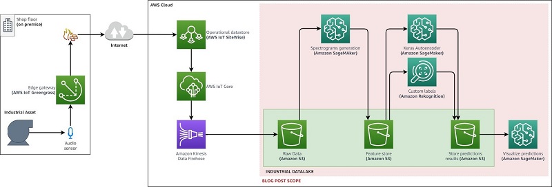
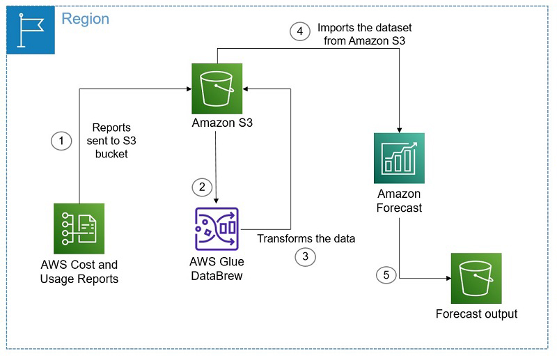
In this post, we implement the area in red of the following architecture. This is a simplified extract of the Connected Factory Solution with AWS IoT. For more information, see Connected Factory Solution based on AWS IoT for Industry 4.0 success.

We walk you through the following steps using the Jupyter notebooks provided with this post:

1. We first focus on data exploration to get familiar with sound data. This data is particular time-series data, and exploring it requires specific approaches.
2. We then use SageMaker to build an autoencoder that we use as a classifier to discriminate between normal and abnormal sounds.
3. We take on a more novel approach in the last part of this post: we transform the sound files into spectrogram images and feed them directly to an image classifier. We use Amazon Rekognition Custom Labels to perform this classification task and leverage SageMaker for the data preprocessing and to drive the Amazon Rekognition Custom Labels training and evaluation process.

Both approaches require an equal amount of effort to complete. Although the models obtained in the end aren’t comparable, this gives you an idea of how much of a kick-start you may get when using an applied AI service.

Introducing the machine sound dataset

You can use the data exploration work available in the first companion notebook from the GitHub repo. The first thing we do is plot the waveforms of normal and abnormal signals (see the following screenshot).

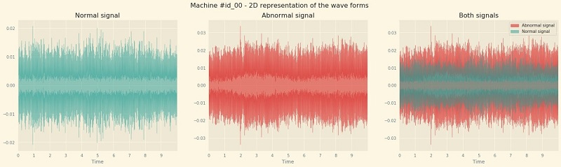
From there, you see how to leverage the short Fourier transformation to build a spectrogram of these signals.

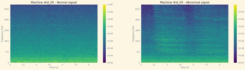
These images have interesting features; this is exactly the kind of features that a neural network can try to uncover and structure. We now build two types of feature extractors based on this data exploration work and feed them to different types of architectures.

Building a custom autoencoder architecture

The autoencoder architecture is a neural network with the same number of neurons in the input and the output layers. This kind of architecture learns to generate the identity transformation between inputs and outputs. The second notebook of our series goes through these different steps:

1. To feed the spectrogram to an autoencoder, build a tabular dataset and upload it to Amazon Simple Storage Service (Amazon S3).
2. Create a TensorFlow autoencoder model and train it in script mode by using the TensorFlow/Keras existing container.
3. Evaluate the model to obtain a confusion matrix highlighting the classification performance between normal and abnormal sounds.

Building the dataset

For this post, we use the librosa library, which is a Python package for audio analysis. A features extraction function based on the steps to generate the spectrogram described earlier is central to the dataset generation process. This feature extraction function is in the sound_tools.py library.

We train our autoencoder only on the normal signals: we want our model to learn how to reconstruct these signals (learning the identity transformation). The main idea is to leverage this for classification later; when we feed this trained model with abnormal sounds, the reconstruction error is a lot higher than when trying to reconstruct normal sounds. We use an error threshold to discriminate abnormal and normal sounds.

Creating the autoencoder

To build our autoencoder, we use Keras and assemble a simple autoencoder architecture with three hidden layers:

from tensorflow.keras import Input
from tensorflow.keras.models import Model
from tensorflow.keras.layers import Dense

def autoencoder_model(input_dims):
    inputLayer = Input(shape=(input_dims,))
    h = Dense(64, activation="relu")(inputLayer)
    h = Dense(64, activation="relu")(h)
    h = Dense(8, activation="relu")(h)
    h = Dense(64, activation="relu")(h)
    h = Dense(64, activation="relu")(h)
    h = Dense(input_dims, activation=None)(h)

    return Model(inputs=inputLayer, outputs=h)

We put this in a training script (model.py) and use the SageMaker TensorFlow estimator to configure our training job and launch the training:

tf_estimator = TensorFlow(
    base_job_name='sound-anomaly',
    entry_point='model.py',
    source_dir='./autoencoder/',
    role=role,
    instance_count=1, 
    instance_type='ml.p3.2xlarge',
    framework_version='2.2',
    py_version='py37',
    hyperparameters={
        'epochs': 30,
        'batch-size': 512,
        'learning-rate': 1e-3,
        'n_mels': n_mels,
        'frame': frames
    },
    debugger_hook_config=False
)

tf_estimator.fit({'training': training_input_path})

Training over 30 epochs takes a few minutes on a p3.2xlarge instance. At this stage, this costs you a few cents. If you plan to use a similar approach on the whole MIMII dataset or use hyperparameter tuning, you can further reduce this training cost by using Managed Spot Training. For more information, see Amazon SageMaker Spot Training Examples.

Evaluating the model

We now deploy the autoencoder behind a SageMaker endpoint:

tf_endpoint_name = 'sound-anomaly-'+time.strftime("%Y-%m-%d-%H-%M-%S", time.gmtime())
tf_predictor = tf_estimator.deploy(
    initial_instance_count=1,
    instance_type='ml.c5.large',
    endpoint_name=tf_endpoint_name
)

This operation creates a SageMaker endpoint that continues to incur costs as long as it’s active. Don’t forget to shut it down at the end of this experiment.

Our test dataset has an equal share of normal and abnormal sounds. We loop through this dataset and send each test file to this endpoint. Because our model is an autoencoder, we evaluate how good the model is at reconstructing the input. The higher the reconstruction error, the greater the chance that we have identified an anomaly. See the following code:

y_true = test_labels
reconstruction_errors = []

for index, eval_filename in tqdm(enumerate(test_files), total=len(test_files)):
    # Load signal
    signal, sr = sound_tools.load_sound_file(eval_filename)

    # Extract features from this signal:
    eval_features = sound_tools.extract_signal_features(
        signal, 
        sr, 
        n_mels=n_mels, 
        frames=frames, 
        n_fft=n_fft, 
        hop_length=hop_length
    )
    
    # Get predictions from our autoencoder:
    prediction = tf_predictor.predict(eval_features)['predictions']
    
    # Estimate the reconstruction error:
    mse = np.mean(np.mean(np.square(eval_features - prediction), axis=1))
    reconstruction_errors.append(mse)

The following plot shows that the distribution of the reconstruction error for normal and abnormal signals differs significantly. The overlap between these histograms means we have to compromise between the metrics we want to optimize for (fewer false positives or fewer false negatives).

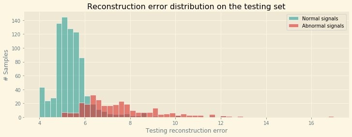
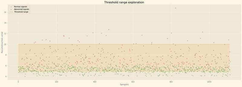
Let’s explore the recall-precision tradeoff for a reconstruction error threshold varying between 5.0–10.0 (this encompasses most of the overlap we can see in the preceding plot). First, let’s visualize how this threshold range separates our signals on a scatter plot of all the testing samples.

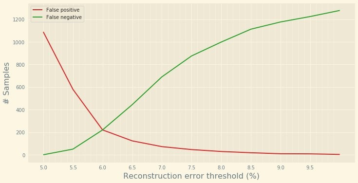
If we plot the number of samples flagged as false positives and false negatives, we can see that the best compromise is to use a threshold set around 6.3 for the reconstruction error (assuming we’re not looking at minimizing either the false positive or false negatives occurrences).

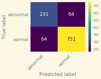
For this threshold (6.3), we obtain the following confusion matrix.

The metrics associated to this matrix are as follows:

• Precision – 92.1%
• Recall – 92.1%
• Accuracy – 88.5%
• F1 score – 92.1%

Cleaning up

Let’s not forget to delete our endpoint to prevent any additional costs by using the delete_endpoint() API.

Autoencoder improvement and further exploration

The spectrogram approach requires defining the spectrogram square dimensions (the number of Mel cell defined in the data exploration notebook), which is a heuristic. In contrast, deep learning networks with a CNN encoder can learn the best representation to perform the task at hand (anomaly detection). The following are further steps to investigate to improve on this first result:

• Experimenting with several more or less complex autoencoder architectures, training for a longer time, performing hyperparameter tuning with different optimizers, or tuning the data preparation sequence (sound discretization parameters).
• Leveraging high-resolution spectrograms and feeding them to a CNN encoder to uncover the most appropriate representation of the sound.
• Using an end-to-end model architecture with an encoder-decoder that have been known to give good results on waveform datasets.
• Using deep learning models with multi-context temporal and channel (eight microphones) attention weights.
• Using time-distributed 2D convolution layers to encode features across the eight channels. You could feed these encoded features as sequences across time steps to an LSTM or GRU layer. From there, multiplicative sequence attention weights can be learnt on the output sequence from the RNN layer.
• Exploring the appropriate image representation for multi-variate time-series signals that aren’t waveform. You could replace spectrograms with Markov transition fields, recurrence plots, or network graphs to achieve the same goals for non-sound time-based signals.

Using Amazon Rekognition Custom Labels

For our second approach, we feed the spectrogram images directly into an image classifier. The third notebook of our series goes through these different steps:

1. Build the datasets. For this use case, we just use images, so we don’t need to prepare tabular data to feed into an autoencoder. We then upload them to Amazon S3.
2. Create an Amazon Rekognition Custom Labels project:
   1. Associate the project with the training data, validation data, and output locations.
   2. Train a project version with these datasets.
3. Start the model. This provisions an endpoint and deploys the model behind it. We can then do the following:
   1. Query the endpoint for inference for the validation and testing datasets.
   2. Evaluate the model to obtain a confusion matrix highlighting the classification performance between normal and abnormal sounds.

Building the dataset

Previously, we had to train our autoencoder on only normal signals. In this use case, we build a more traditional split of training and testing datasets. Based on the fans sound database, this yields the following:

• 4,390 signals for the training dataset, including 3,210 normal signals and 1,180 abnormal signals
• 1,110 signals for the testing dataset, including 815 normal signals and 295 abnormal signals

We generate and store the spectrogram of each signal and upload them in either a train or test bucket.

Creating an Amazon Rekognition Custom Labels model

The first step is to create a project with the Rekognition Custom Labels boto3 API:

# Initialization, get a Rekognition client:
PROJECT_NAME = 'sound-anomaly-detection'
reko_client = boto3.client("rekognition")

# Let's try to create a Rekognition project:
try:
    project_arn = reko_client.create_project(ProjectName=PROJECT_NAME)['ProjectArn']
    
# If the project already exists, we get its ARN:
except reko_client.exceptions.ResourceInUseException:
    # List all the existing project:
    print('Project already exists, collecting the ARN.')
    reko_project_list = reko_client.describe_projects()
    
    # Loop through all the Rekognition projects:
    for project in reko_project_list['ProjectDescriptions']:
        # Get the project name (the string after the first delimiter in the ARN)
        project_name = project['ProjectArn'].split('/')[1]
        
        # Once we find it, we store the ARN and break out of the loop:
        if (project_name == PROJECT_NAME):
            project_arn = project['ProjectArn']
            break
            
print(project_arn)

We need to tell Amazon Rekognition where to find the training data and testing data, and where to output its results:

TrainingData = {
    'Assets': [{ 
        'GroundTruthManifest': {
            'S3Object': { 
                'Bucket': BUCKET_NAME,
                'Name': f'{PREFIX_NAME}/manifests/train.manifest'
            }
        }
    }]
}

TestingData = {
    'AutoCreate': True
}

OutputConfig = { 
    'S3Bucket': BUCKET_NAME,
    'S3KeyPrefix': f'{PREFIX_NAME}/output'
}

Now we can create a project version. Creating a project version builds and trains a model within this Amazon Rekognition project for the data previously configured. Project creation can fail if Amazon Rekognition can’t access the bucket you selected. Make sure the right bucket policy is applied to your bucket (check the notebooks to see the recommended policy).

The following code launches a new model training, and you have to wait approximately 1 hour (less than $1 from a cost perspective) for the model to be trained:

version = 'experiment-1'
VERSION_NAME = f'{PROJECT_NAME}.{version}'

# Let's try to create a new project version in the current project:
try:
    project_version_arn = reko_client.create_project_version(
        ProjectArn=project_arn,      # Project ARN
        VersionName=VERSION_NAME,    # Name of this version
        OutputConfig=OutputConfig,   # S3 location for the output artefact
        TrainingData=TrainingData,   # S3 location of the manifest describing the training data
        TestingData=TestingData      # S3 location of the manifest describing the validation data
    )['ProjectVersionArn']
    
# If a project version with this name already exists, we get its ARN:
except reko_client.exceptions.ResourceInUseException:
    # List all the project versions (=models) for this project:
    print('Project version already exists, collecting the ARN:', end=' ')
    reko_project_versions_list = reko_client.describe_project_versions(ProjectArn=project_arn)
    
    # Loops through them:
    for project_version in reko_project_versions_list['ProjectVersionDescriptions']:
        # Get the project version name (the string after the third delimiter in the ARN)
        project_version_name = project_version['ProjectVersionArn'].split('/')[3]

        # Once we find it, we store the ARN and break out of the loop:
        if (project_version_name == VERSION_NAME):
            project_version_arn = project_version['ProjectVersionArn']
            break
            
print(project_version_arn)
status = reko_client.describe_project_versions(
    ProjectArn=project_arn,
    VersionNames=[project_version_arn.split('/')[3]]
)['ProjectVersionDescriptions'][0]['Status']

Deploying and evaluating the model

First, we deploy our model by using the ARN collected earlier (see the following code). This deploys an endpoint that costs you around $4 per hour. Don’t forget to decommission it when you’re done.

# Start the model
print('Starting model: ' + model_arn)
response = reko_client.start_project_version(ProjectVersionArn=model_arn, MinInferenceUnits=min_inference_units)

# Wait for the model to be in the running state:
project_version_running_waiter = client.get_waiter('project_version_running')
project_version_running_waiter.wait(ProjectArn=project_arn, VersionNames=[version_name])

# Get the running status
describe_response=client.describe_project_versions(ProjectArn=project_arn, VersionNames=[version_name])
for model in describe_response['ProjectVersionDescriptions']:
    print("Status: " + model['Status'])
    print("Message: " + model['StatusMessage'])

When the model is running, you can start querying it for predictions. The notebook contains the function get_results(), which queries a given model with a list of pictures sitting in a given path. This takes a few minutes to run all the test samples and costs less than $1 (for approximately 3,000 test samples). See the following code:

predictions_ok = rt.get_results(project_version_arn, BUCKET, s3_path=f'{BUCKET}/{PREFIX}/test/normal', label='normal', verbose=True)
predictions_ko = rt.get_results(project_version_arn, BUCKET, s3_path=f'{BUCKET}/{PREFIX}/test/abnormal', label='abnormal', verbose=True)

def get_results(project_version_arn, bucket, s3_path, label=None, verbose=True):
    """
    Sends a list of pictures located in an S3 path to
    the endpoint to get the associated predictions.
    """

    fs = s3fs.S3FileSystem()
    data = {}
    predictions = pd.DataFrame(columns=['image', 'normal', 'abnormal'])
    
    for file in fs.ls(path=s3_path, detail=True, refresh=True):
        if file['Size'] > 0:
            image = '/'.join(file['Key'].split('/')[1:])
            if verbose == True:
                print('.', end='')

            labels = show_custom_labels(project_version_arn, bucket, image, 0.0)
            for L in labels:
                data[L['Name']] = L['Confidence']
                
            predictions = predictions.append(pd.Series({
                'image': file['Key'].split('/')[-1],
                'abnormal': data['abnormal'],
                'normal': data['normal'],
                'ground truth': label
            }), ignore_index=True)
            
    return predictions
    
def show_custom_labels(model, bucket, image, min_confidence):
    # Call DetectCustomLabels from the Rekognition API: this will give us the list 
    # of labels detected for this picture and their associated confidence level:
    reko_client = boto3.client('rekognition')
    try:
        response = reko_client.detect_custom_labels(
            Image={'S3Object': {'Bucket': bucket, 'Name': image}},
            MinConfidence=min_confidence,
            ProjectVersionArn=model
        )
        
    except Exception as e:
        print(f'Exception encountered when processing {image}')
        print(e)
        
    # Returns the list of custom labels for the image passed as an argument:
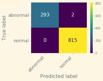
    return response['CustomLabels']

Let’s plot the confusion matrix associated to this test set (see the following diagram).

The metrics associated to this matrix are as follows:

• Precision – 100.0%
• Recall – 99.8%
• Accuracy – 99.8%
• F1 score – 99.9%

Without much effort (and no ML knowledge!), we can get impressive results. With such a low false negative rate and without any false positives, we can leverage such a model in even the most challenging industrial context.

Cleaning up

We need to stop the running model to avoid incurring costs while the endpoint is live:

response = reko_client.stop_project_version(ProjectVersionArn=model_arn)

Results comparison

Let’s display the results side by side. The following matrix shows the unsupervised custom TensorFlow model, and an F1 score of 92.1%.

The data preparation effort includes the following:

• No need to collect abnormal signals; only the normal signal is used to build the training dataset
• Generating spectrograms
• Building sequences of sound frames
• Building training and testing datasets
• Uploading datasets to the S3 bucket

The modeling and improvement effort include the following:

• Designing the autoencoder architecture
• Writing a custom training script
• Writing the distribution code (to ensure scalability)
• Performing hyperparameter tuning

The following matrix shows the supervised custom Amazon Rekognition Custom Labels model, and an F1 score of 99.9%.

The data preparation effort includes the following:

• Collecting a balanced dataset with enough abnormal signals
• Generating spectrograms
• Making the train and test split
• Uploading spectrograms to the respective S3 training and testing buckets

The modeling and improvement effort include the following:

• None! 

Determining which approach to use

Which approach should you use? You might use both! As expected, using a supervised approach yields better results. However, the unsupervised approach is perfect to start curating your collected data to easily identify abnormal situations. When you have enough abnormal signals to build a more balanced dataset, you can switch to the supervised approach. Your overall process looks something like the following:

1. Start collecting the sound data.
2. When you have enough data, train an unsupervised model and use the results to start issuing warnings to a pilot team, who annotates (confirms) abnormal conditions and sets them aside.
3. When you have enough data characterizing abnormal conditions, train a supervised model.
4. Deploy the supervised approach to a larger scale (especially if you can tune it to limit the undesired false negative to a minimum number).
5. Continue collecting sound signals for normal and abnormal conditions, and monitor potential drift between the recent data and the one used for training. Optionally, you can also further detail the anomalies to detect different types of abnormal conditions.

Conclusion

A major challenge factory managers have in order to take advantage of the most recent progress in AI and ML is the amount of customization needed. Training anomaly detection models that can be adapted to many different industrial machineries in order to reduce the maintenance effort, reduce rework or waste, increase product quality, or improve overall equipment efficiency (OEE) or product lines is a massive amount of work.

SageMaker and Amazon Applied AI services such as Amazon Rekognition Custom Labels enables manufacturers to build AI models without having access to a versatile team of data scientists sitting next to each production line. These services allow you to focus on collecting good quality data to augment your factory and provide machine operators, process engineers, and lean manufacturing practioners with high quality insights.

Building upon this solution, you could record 10 seconds sound snippets of your machines and send them to the cloud every 5 minutes, for instance. After you train a model, you can use its predictions to feed custom notifications that you can send back to the supervision screens sitting in the factory.

Can you apply the same process to actual time series as captured by machine sensors? In these cases, spectrograms might not be the best visual representation for these. What about multivariate time series? How can we generalize this approach? Stay tuned for future posts and samples on this impactful topic!

If you’re an ML practitioner passionate about industrial use cases, head over to the Performing anomaly detection on industrial equipment using audio signals GitHub repo for more examples. The solution in this post features an industrial use case, but you can use sound classification ML models in a variety of other settings, for example to analyze animal behavior in agriculture, or to detect anomalous urban sounds such as gunshots, accidents, or dangerous driving. Don’t hesitate to test these services, and let us know what you built!

About the Author

Michaël Hoarau is an AI/ML specialist solution architect at AWS who alternates between a data scientist and machine learning architect, depending on the moment. He is passionate about bringing the power of AI/ML to the shop floors of his industrial customers and has worked on a wide range of ML use cases, ranging from anomaly detection to predictive product quality or manufacturing optimization. When not helping customers develop the next best machine learning experiences, he enjoys observing the stars, traveling, or playing the piano.

Read More

AWS Cost Explorer enables you to view and analyze your AWS Cost and Usage Reports (AWS CUR). You can also predict your overall cost associated with AWS services in the future by creating a forecast of AWS Cost Explorer, but you can’t view historical data beyond 12 months. Moreover, running custom machine learning (ML) models on historical data can be labor and knowledge intensive, often requiring some programming language for data transformation and building models.

In this post, we show you how to use Amazon Forecast, a fully managed service that uses ML to deliver highly accurate forecasts, with data collected from AWS CUR. AWS Glue DataBrew is a new visual data preparation tool that makes it easy for data analysts and data scientists to clean and normalize data to prepare it for analytics and ML. We can use DataBrew to transform CUR data into the appropriate dataset format, which Forecast can later ingest to train a predictor and create a forecast. We can transform the data into the required format and predict the cost for a given service or member account ID without writing a single line of code.

The following is the architecture diagram of the solution.

Walkthrough

You can choose hourly, daily, or monthly reports that break out costs by product or resource (including self-defined tags) using the AWS CUR. AWS delivers the CUR to an Amazon Simple Storage Service (Amazon S3) bucket, where this data is securely retained and accessible. Because cost and usage data are timestamped, you can easily deliver the data to Forecast. In this post, we use CUR data that is collected on a daily basis. After you set up the CUR, you can use DataBrew to transform the CUR data into the appropriate format for Forecast to train a predictor and create a forecast output without writing a single line of code. In this post, we walk you through the following high-level tasks:

1. Prepare the data.
2. Transform the data.
3. Prepare the model.
4. Validate the predictors.
5. Generate a forecast.

Prerequisites

Before we begin, let’s create an S3 bucket to store the results from the DataBrew job. Remember the bucket name, because we refer to this bucket during deployment. With DataBrew, you can determine the transformations and then schedule them to run automatically on new daily, weekly, or monthly data as it comes in without having to repeat the data preparation manually.

Preparing the data

To prepare your data, complete the following steps:

1. On the DataBrew console, create a new project.
2. For Select a dataset, select New dataset.

When selecting CUR data, you can select a single object, or the contents of an entire folder.

If you don’t have substantial or interesting usage in your report, you can use a sample file available on Verify Your CUR Files Are Being Delivered. Make sure you follow the folder structure when uploading the Parquet files, and make sure the folder only contains the Parquet files needed. If the folder has other random files, it errors out.

3. Create a role in AWS Identity and Access Management (IAM) that allows DataBrew to access CUR files.

You can either create a custom role or have DataBrew create one on your behalf.

4. Choose Create project.

DataBrew takes you to the the project screen to view and analyze your data.

First, we need to select only those columns required for Forecast. We can do this by grouping the columns by our desired dimensions and creating a summed column of unblended costs.

5. Choose the Group icon on the navigation bar and group by the following columns:
   1. line_item_usage_start_date, GROUP BY
   2. product_product_name, GROUP BY
   3. line_item_usage_account_id, GROUP BY
   4. line_item_unblended_cost, SUM

6. For Group type, select Group as new table to replace all existing columns with new columns.

This extracts only the required columns for our forecast.

7. Choose Finish.

In DataBrew, a recipe is a set of data transformation steps. As you progress, DataBrew documents your data transformation steps. You can save and use these recipes in the future for new datasets and transformation iterations.

8. Choose Add step.
9. For Create column options¸ choose Based on functions.
10. For Select a function, choose DATEFORMAT.
11. For Values using, choose Source column.
12. For Source column, choose line_item_usage_start_date.
13. For Date format, choose yyyy-mm-dd.

14. Add a destination column of your choice.
15. Choose Apply.

We can delete the original timestamp column because it’s a duplicate.

16. Choose Add step.
17. Delete the original line_item_usage_start_date column.
18. Choose Apply.

Finally, let’s change our summed cost column to a numeric data type.

19. Choose the Setting icon for the line_item_unblended_cost_sum column.
20. For Change type to, choose # number.
21. Choose Apply.

DataBrew documented all four steps of this recipe. You can version recipes as your analytical needs change.

22. Choose Publish to publish an initial version of the recipe.

Transforming the data

Now that we have finished all necessary steps to transform our data, we can instruct DataBrew to run the actual transformation and output the results into an S3 bucket.

1. On the DataBrew project page, choose Create job.
2. For Job name, enter a name for your job.
3. Under Job output settings¸ for File type¸ choose CSV.
4. For S3 location, enter the S3 bucket we created in the prerequisites.

5. Choose either the IAM role you created or the one DataBrew created for you.
6. Choose Run job.

It may take several minutes for the job to complete. When it’s complete, navigate to the Amazon S3 console and choose the S3 bucket to find the results. The bucket contains multiple CSV files with keys starting with _part0000.csv. As a fully managed service, DataBrew can run jobs in parallel on multiple nodes to process large files on your behalf. This isn’t a problem because you can specify an entire folder for Forecast to process.

Scheduling DataBrew jobs

You can schedule DataBrew jobs to transform the CUR to update to provide Forecast with a refreshed dataset.

1. On the Job menu, choose the Schedules tab.
2. Provide a schedule name.
3. Specify the run frequency on the day and hour.
4. Optionally, provide the start time for the job run.

DataBrew then runs the job per your configuration.

Preparing the model

To prepare your model, complete the following steps:

1. On the Forecast console, choose Dataset groups.
2. Choose Create dataset group.
3. For Dataset group name, enter a name.
4. For Forecasting domain, choose Custom.
5. Choose Next.

We need to create a target time series dataset.

6. For Frequency of data, choose 1 day.

We can define the data schema to help Forecast become aware of our data types.

7. Drag the timestamp attribute name column to the top of the list.
8. For Timestamp Format, choose yyyy-MM-dd. 

This aligns to the data transformation step we completed in DataBrew.

9. Add an attribute as the third column with the name as account_id and attribute type as string.

10. For Dataset import name, enter a name.
11. For Select time zone, choose your time zone.
12. For Data location, enter the path to the files in your S3 bucket.

If you browse Amazon S3 for the data location, you can only choose individual files. Because our DataBrew output consists of multiple files, enter the S3 path to the files’ location and make sure that a slash (/) is at the end of the path.

13. For IAM role, you can create a role so Forecast has permissions to only access the S3 bucket containing the DataBrew output.
14. Choose Start import.

Forecast takes approximately 45 minutes to import your data. You can view the status of your import on the Datasets page.

15. When the latest import status shows as Active, proceed with training a predictor.
16. For Predictor name, enter a name.
17. For Forecast horizon, enter a number that tells Forecast how far into the future to predict your data.

The forecast horizon can’t exceed one-third length of the target time series.

18. For Forecast frequency, leave at 1 day.
19. If you’re unsure of which algorithm to use to train your model, for Algorithm selection, select Automatic (AutoML). 

This option lets Forecast select the optimal algorithm for your datasets, which automatically trains a model and provides accuracy metrics and generate forecasts. Otherwise, you can manually select one of the built-in algorithms. For this post, we use AutoML.

20. For Forecast dimension, choose account_id.

This allows Forecast to predict cost by account ID in addition to product name.

21. Leave all other options at their default and choose Train predictor.

Forecast begins training the optimal ML model on your dataset. This could take up to an hour to complete. You can check on the training status on the Predictors page. You can generate a forecast after the predictor training status shows as Active.

When it’s complete, you can see that Forecast chose DeepAR+ as the optimal ML algorithm. DeepAR+ analyzes the data as similar time series across a set of cross-functional units. These time series groupings demand different product names and account IDs. In this case, it can be beneficial to train a single model jointly over all time series.

Validating the predictors

Forecast provides comprehensive accuracy metrics to help you understand the performance of your forecasting model, and can compare it to the previous forecasting models you’ve created that may have looked at a different set of variables or used a different period of time for the historical data.

By validating our predictors, we can measure the accuracy of forecasts for individual items. In the Algorithm metrics section on the predictor details page, you can view the accuracy metrics of the predictor, which include the following:

• WQL – Weighted quantile loss at a given quantile
• WAPE – Weighted absolute percentage error
• RMSE – Root mean square error

As another method, we can export the accuracy metrics and forecasted values using algorithm metrics for our predictor. With this method, you can view accuracy metrics for specific services when forecasting, such as Amazon Elastic Compute Cloud (Amazon EC2) or Amazon Relational Database Service (Amazon RDS).

1. Select the predictor you created.
2. Choose Export backtest results.
3. For Export name¸ enter a name.
4. For IAM role¸ choose the role you used earlier.
5. For S3 predictor backtest export location, enter the S3 path where you want Forecast to export the accuracy metrics and forecasted values.

6. Choose Create predictor backtest report.

After some time, Forecast delivers the export results to the S3 location you specified. Forecast exports two files to Amazon S3 in two different folders: forecasted-values and accuracy-metric-values. For more information about accuracy metrics, see Amazon Forecast now supports accuracy measurements for individual items. 

Generating a forecast

To create a forecast, complete the following steps:

1. For Forecast name, enter a name.
2. For Predictor¸ choose the predictor you created.
3. For Forecast types, you can specify up to five quantile values. For this post, we leave it blank to use the defaults.
4. Choose Create new forecast.

When it’s complete, the forecast status shows as Active. Let’s now create a forecast lookup.

5. For Forecast¸ choose the forecast you just created.
6. Specify the start and end date within the bounds of the forecast.
7. For Value, enter a service name (for this post, Amazon RDS).
8. Choose Get Forecast.

Forecast returns P10, P50, and P90 estimates as the default lower, middle, and upper bounds, respectively. For more information about predictor metrics, see Evaluating Predictor Accuracy. Feel free to explore different forecasts for different services in addition to creating a forecast for account ID.

Congratulations! You’ve just created a solution to retrieve forecasts on your CUR by using Amazon S3, DataBrew, and Forecast without writing a single line of code. With these services, you only pay for what you use and don’t have to worry about managing the underlying infrastructure to run transformations and ML inferences. 

Conclusion

In this post, we illustrated how to use DataBrew to transform the CUR into a format for Forecast to make predictions without any need for ML expertise. We created datasets, predictors, and a forecast, and used Forecast to predict costs for specific AWS services. To get started with Amazon Forecast, visit the product page. We also recently announced that CUR is available to member (linked) accounts. Now any entity with the proper permissions under any account within an AWS organization can use the CUR to view and manage costs.

About the Authors

Jyoti Tyagi is a Solutions Architect with great passion for artificial intelligence and machine learning. She helps customers to architect highly secured and well-architected applications on the AWS Cloud with best practices. In her spare time, she enjoys painting and meditation.

Peter Chung is a Solutions Architect for AWS, and is passionate about helping customers uncover insights from their data. He has been building solutions to help organizations make data-driven decisions in both the public and private sectors. Outside of work, he enjoys cooking and spending time with his family.

Read More

With the rapid adoption of machine learning (ML) and MLOps, enterprises want to increase the velocity of ML projects from experimentation to production.

During the initial phase of an ML project, data scientists collaborate and share experiment results in order to find a solution to a business need. During the operational phase, you also need to manage the different model versions going to production and your lifecycle. In this post, we’ll show how the open-source platform MLflow helps address these issues. For those interested in a fully managed solution, Amazon Web Services recently announced Amazon SageMaker Pipelines at re:Invent 2020, the first purpose-built, easy-to-use continuous integration and continuous delivery (CI/CD) service for machine learning (ML). You can learn more about SageMaker Pipelines in this post.

MLflow is an open-source platform to manage the ML lifecycle, including experimentation, reproducibility, deployment, and a central model registry. It includes the following components:

• Tracking – Record and query experiments: code, data, configuration, and results
• Projects – Package data science code in a format to reproduce runs on any platform
• Models – Deploy ML models in diverse serving environments
• Registry – Store, annotate, discover, and manage models in a central repository

The following diagram illustrates our architecture.

In the following sections, we show how to deploy MLflow on AWS Fargate and use it during your ML project with Amazon SageMaker. We use SageMaker to develop, train, tune, and deploy a Scikit-learn based ML model (random forest) using the Boston House Prices dataset. During our ML workflow, we track experiment runs and our models with MLflow.

SageMaker is a fully managed service that provides developers and data scientists the ability to build, train, and deploy ML models quickly. SageMaker removes the heavy lifting from each step of the ML process to make it easier to develop high-quality models.

Walkthrough overview

This post demonstrates how to do the following:

• Host a serverless MLflow server on Fargate
• Set Amazon Simple Storage Service (Amazon S3) and Amazon Relational Database Service (Amazon RDS) as artifact and backend stores, respectively
• Track experiments running on SageMaker with MLflow
• Register models trained in SageMaker in the MLflow Model Registry
• Deploy an MLflow model into a SageMaker endpoint

The detailed step-by-step code walkthrough is available in the GitHub repo.

Architecture overview

You can set up a central MLflow tracking server during your ML project. You use this remote MLflow server to manage experiments and models collaboratively. In this section, we show you how you can Dockerize your MLflow tracking server and host it on Fargate.

An MLflow tracking server also has two components for storage: a backend store and an artifact store.

We use an S3 bucket as our artifact store and an Amazon RDS for MySQL instance as our backend store.

The following diagram illustrates this architecture.

Running an MLflow tracking server on a Docker container

You can install MLflow using pip install mlflow and start your tracking server with the mlflow server command.

By default, the server runs on port 5000, so we expose it in our container. Use 0.0.0.0 to bind to all addresses if you want to access the tracking server from other machines. We install boto3 and pymysql dependencies for the MLflow server to communicate with the S3 bucket and the RDS for MySQL database. See the following code:

FROM python:3.8.0

RUN pip install 
    mlflow 
    pymysql 
    boto3 & 
    mkdir /mlflow/

EXPOSE 5000

## Environment variables made available through the Fargate task.
## Do not enter values
CMD mlflow server 
    --host 0.0.0.0 
    --port 5000 
    --default-artifact-root ${BUCKET} 
    --backend-store-uri mysql+pymysql://${USERNAME}:${PASSWORD}@${HOST}:${PORT}/${DATABASE}

Hosting an MLflow tracking server with Fargate

In this section, we show how you can run your MLflow tracking server on a Docker container that is hosted on Fargate.

Fargate is an easy way to deploy your containers on AWS. It allows you to use containers as a fundamental compute primitive without having to manage the underlying instances. All you need is to specify an image to deploy and the amount of CPU and memory it requires. Fargate handles updating and securing the underlying Linux OS, Docker daemon, and Amazon Elastic Container Service (Amazon ECS) agent, as well as all the infrastructure capacity management and scaling.

For more information about running an application on Fargate, see Building, deploying, and operating containerized applications with AWS Fargate.

The MLflow container first needs to be built and pushed to an Amazon Elastic Container Registry (Amazon ECR) repository. The container image URI is used at registration of our Amazon ECS task definition. The ECS task has an AWS Identity and Access Management (IAM) role attached to it, allowing it to interact with AWS services such as Amazon S3.

The following screenshot shows our task configuration.

The Fargate service is set up with autoscaling and a network load balancer so it can adjust to the required compute load with minimal maintenance effort on our side.

When running our ML project, we set mlflow.set_tracking_uri(<load balancer uri>) to interact with the MLflow server via the load balancer.

Using Amazon S3 as the artifact store and Amazon RDS for MySQL as backend store

The artifact store is suitable for large data (such as an S3 bucket or shared NFS file system) and is where clients log their artifact output (for example, models). MLflow natively supports Amazon S3 as artifact store, and you can use --default-artifact-root ${BUCKET} to refer to the S3 bucket of your choice.

The backend store is where MLflow Tracking Server stores experiments and runs metadata, as well as parameters, metrics, and tags for runs. MLflow supports two types of backend stores: file store and database-backed store. It’s better to use an external database-backed store to persist the metadata.

As of this writing, you can use databases such as MySQL, SQLite, and PostgreSQL as a backend store with MLflow. For more information, see Backend Stores.

Amazon Aurora is a MySQL and PostgreSQL-compatible relational database and can also be used for this.

For this example, we set up an RDS for MySQL instance. Amazon RDS makes it easy to set up, operate, and scale MySQL deployments in the cloud. With Amazon RDS, you can deploy scalable MySQL servers in minutes with cost-efficient and resizable hardware capacity.

You can use --backend-store-uri mysql+pymysql://${USERNAME}:${PASSWORD}@${HOST}:${PORT}/${DATABASE} to refer MLflow to the MySQL database of your choice.

Launching the example MLflow stack

To launch your MLflow stack, follow these steps:

1. Launch the AWS CloudFormation stack provided in the GitHub repo
2. Choose Next.
3. Leave all options as default until you reach the final screen.
4. Select I acknowledge that AWS CloudFormation might create IAM resources.
5. Choose Create.

The stack takes a few minutes to launch the MLflow server on Fargate, with an S3 bucket and a MySQL database on RDS. The load balancer URI is available on the Outputs tab of the stack.

You can then use the load balancer URI to access the MLflow UI.

In this illustrative example stack, our load balancer is launched on a public subnet and is internet facing.

For security purposes, you may want to provision an internal load balancer in your VPC private subnets where there is no direct connectivity from the outside world. For more information, see Access Private applications on AWS Fargate using Amazon API Gateway PrivateLink.

Tracking SageMaker runs with MLflow

You now have a remote MLflow tracking server running accessible through a REST API via the load balancer URI.

You can use the MLflow Tracking API to log parameters, metrics, and models when running your ML project with SageMaker. For this you need to install the MLflow library when running your code on SageMaker and set the remote tracking URI to be your load balancer address.

The following Python API command allows you to point your code running on SageMaker to your MLflow remote server:

import mlflow
mlflow.set_tracking_uri('<YOUR LOAD BALANCER URI>')

Connect to your notebook instance and set the remote tracking URI. The following diagram shows the updated architecture.

Managing your ML lifecycle with SageMaker and MLflow

You can follow this example lab by running the notebooks in the GitHub repo.

This section describes how to develop, train, tune, and deploy a random forest model using Scikit-learn with the SageMaker Python SDK. We use the Boston Housing dataset, present in Scikit-learn, and log our ML runs in MLflow.

You can find the original lab in the SageMaker Examples GitHub repo for more details on using custom Scikit-learn scripts with SageMaker.

Creating an experiment and tracking ML runs

In this project, we create an MLflow experiment named boston-house and launch training jobs for our model in SageMaker. For each training job run in SageMaker, our Scikit-learn script records a new run in MLflow to keep track of input parameters, metrics, and the generated random forest model.

The following example API calls can help you start and manage MLflow runs:

• start_run() – Starts a new MLflow run, setting it as the active run under which metrics and parameters are logged
• log_params() – Logs a parameter under the current run
• log_metric() – Logs a metric under the current run
• sklearn.log_model() – Logs a Scikit-learn model as an MLflow artifact for the current run

For a complete list of commands, see MLflow Tracking.

The following code demonstrates how you can use those API calls in your train.py script:

# set remote mlflow server
mlflow.set_tracking_uri(args.tracking_uri)
mlflow.set_experiment(args.experiment_name)

with mlflow.start_run():
    params = {
        "n-estimators": args.n_estimators,
        "min-samples-leaf": args.min_samples_leaf,
        "features": args.features
    }
    mlflow.log_params(params)
    
    # TRAIN
    logging.info('training model')
    model = RandomForestRegressor(
        n_estimators=args.n_estimators,
        min_samples_leaf=args.min_samples_leaf,
        n_jobs=-1
    )

    model.fit(X_train, y_train)

    # ABS ERROR AND LOG COUPLE PERF METRICS
    logging.info('evaluating model')
    abs_err = np.abs(model.predict(X_test) - y_test)

    for q in [10, 50, 90]:
        logging.info(f'AE-at-{q}th-percentile: {np.percentile(a=abs_err, q=q)}')
        mlflow.log_metric(f'AE-at-{str(q)}th-percentile', np.percentile(a=abs_err, q=q))

    # SAVE MODEL
    logging.info('saving model in MLflow')
    mlflow.sklearn.log_model(model, "model")

Your train.py script needs to know which MLflow tracking_uri and experiment_name to use to log the runs. You can pass those values to your script using the hyperparameters of the SageMaker training jobs. See the following code:

# uri of your remote mlflow server
tracking_uri = '<YOUR LOAD BALANCER URI>' 
experiment_name = 'boston-house'

hyperparameters = {
    'tracking_uri': tracking_uri,
    'experiment_name': experiment_name,
    'n-estimators': 100,
    'min-samples-leaf': 3,
    'features': 'CRIM ZN INDUS CHAS NOX RM AGE DIS RAD TAX PTRATIO B LSTAT',
    'target': 'target'
}

estimator = SKLearn(
    entry_point='train.py',
    source_dir='source_dir',
    role=role,
    metric_definitions=metric_definitions,
    hyperparameters=hyperparameters,
    train_instance_count=1,
    train_instance_type='local',
    framework_version='0.23-1',
    base_job_name='mlflow-rf',
)

Performing automatic model tuning with SageMaker and tracking with MLflow

SageMaker automatic model tuning, also known as Hyperparameter Optimization (HPO), finds the best version of a model by running many training jobs on your dataset using the algorithm and ranges of hyperparameters that you specify. It then chooses the hyperparameter values that result in a model that performs the best, as measured by a metric that you choose.

In the 2_track_experiments_hpo.ipynb example notebook, we show how you can launch a SageMaker tuning job and track its training jobs with MLflow. It uses the same train.py script and data used in single training jobs, so you can accelerate your hyperparameter search for your MLflow model with minimal effort.

When the SageMaker jobs are complete, you can navigate to the MLflow UI and compare results of different runs (see the following screenshot).

This can be useful to promote collaboration within your development team.

Managing models trained with SageMaker using the MLflow Model Registry

The MLflow Model Registry component allows you and your team to collaboratively manage the lifecycle of a model. You can add, modify, update, transition, or delete models created during the SageMaker training jobs in the Model Registry through the UI or the API.

In your project, you can select a run with the best model performance and register it into the MLflow Model Registry. The following screenshot shows example registry details.

After a model is registered, you can navigate to the Registered Models page and view its properties.

Deploying your model in SageMaker using MLflow

This sections shows how to use the mlflow.sagemaker module provided by MLflow to deploy a model into a SageMaker-managed endpoint. As of this writing, MLflow only supports deployments to SageMaker endpoints, but you can use the model binaries from the Amazon S3 artifact store and adapt them to your deployment scenarios.

Next, you need to build a Docker container with inference code and push it to Amazon ECR.

You can build your own image or use the mlflow sagemaker build-and-push-container command to have MLflow create one for you. This builds an image locally and pushes it to an Amazon ECR repository called mlflow-pyfunc.

The following example code shows how to use mlflow.sagemaker.deploy to deploy your model into a SageMaker endpoint:

# URL of the ECR-hosted Docker image the model should be deployed into
image_uri = '<YOUR mlflow-pyfunc ECR IMAGE URI>'
endpoint_name = 'boston-housing'
# The location, in URI format, of the MLflow model to deploy to SageMaker.
model_uri = '<YOUR MLFLOW MODEL LOCATION>'

mlflow.sagemaker.deploy(
    mode='create',
    app_name=endpoint_name,
    model_uri=model_uri,
    image_url=image_uri,
    execution_role_arn=role,
    instance_type='ml.m5.xlarge',
    instance_count=1,
    region_name=region
)

The command launches a SageMaker endpoint into your account, and you can use the following code to generate predictions in real time:

# load boston dataset
data = load_boston()
df = pd.DataFrame(data.data, columns=data.feature_names)

runtime= boto3.client('runtime.sagemaker')
# predict on the first row of the dataset
payload = df.iloc[[0]].to_json(orient="split")

runtime_response = runtime.invoke_endpoint(EndpointName=endpoint_name, ContentType='application/json', Body=payload)
result = json.loads(runtime_response['Body'].read().decode())
print(f'Payload: {payload}')
print(f'Prediction: {result}')

Current limitation on user access control

As of this writing, the open-source version of MLflow doesn’t provide user access control features in case you have multiple tenants on your MLflow server. This means any user with access to the server can modify experiments, model versions, and stages. This can be a challenge for enterprises in regulated industries that need to keep strong model governance for audit purposes.

Summary

In this post, we covered how you can host an open-source MLflow server on AWS using Fargate, Amazon S3, and Amazon RDS. We then showed an example ML project lifecycle of tracking SageMaker training and tuning jobs with MLflow, managing model versions in the MLflow Model Registry, and deploying an MLflow model into a SageMaker endpoint for prediction. Try out the solution on your own by accessing the GitHub repo and let us know if you have any questions in the comments!

About the Authors

Sofian Hamiti is an AI/ML specialist Solutions Architect at AWS. He helps customers across industries accelerate their AI/ML journey by helping them build and operationalize end-to-end machine learning solutions.

Shreyas Subramanian is a Principal AI/ML specialist Solutions Architect, and helps Manufacturing, Industrial, Automotive and Aerospace customers build Machine Learning and optimization related architectures to solve their business challenges using the AWS platform.

Read More

One of the challenging parts of machine learning (ML) is feature engineering, the process of transforming data to create features for ML. Features are processed data signals used for training ML models and for deployed models to make accurate predictions. Data scientists and ML engineers can spend up to 60-70% of their time on feature engineering. It’s also typical to have this work repeated by different teams within an organization who use the same data to build ML models for different solutions, further increasing effort levels for feature engineering. Moreover, it’s important that the generated features should be available for both training and real-time inference use cases, to ensure consistency between model training and inference serving.

A purpose-built feature store for ML is needed to ensure both high-quality ML predictions with a consistent set of features, and cost reduction by eliminating duplicate feature engineering effort and storage overhead. Consistent features are needed between different parts of an organization, and between training and inference for any given ML model. There is also a need for feature stores to meet the high performance, scale, and availability requirements to serve features in near-real time for inferences. Because of this, organizations are often forced to do the heavy lifting of building and maintaining feature store systems, which can become expensive and difficult to maintain.

At AWS we are constantly listening to our customers and building solutions and services that delight them. We heard from many customers about the pain their data science and data engineering teams face when managing features, and used those inputs to build the Amazon SageMaker Feature Store, which was launched at re:Invent on December 1, 2020. Amazon SageMaker Feature Store is a fully managed, purpose-built repository to securely store, update, retrieve, and share ML features.

Although there is a lot to unpack in terms of the capabilities that SageMaker Feature Store brings to the table, in this post, we focus on key capabilities for data ingestion, data access, and security and access control.

Overview of SageMaker Feature Store

As a purpose-built feature store for ML, SageMaker Feature Store is designed to enable you to do the following:

• Securely store and serve features for real-time and batch applications – SageMaker Feature Store serves features at a very low latency for real-time use-cases. It enables you to use ML to make near-real time decisions by enabling feature vector retrievals with low millisecond latencies (p95 latency lower than 10 milliseconds for a 15-kilobyte payload).
• Accelerate model development by sharing and reusing features – Feature engineering is a long and tedious process that often gets repeated by multiple teams within an organization working on the same data. SageMaker Feature Store enables data scientists to spend less time on data preparation and feature computation, and more time on ML innovation, by letting them discover and reuse existing engineered features across the organization.
• Provide historical data access – Features are used for training purposes, and a good feature store should provide easy and quick access to historical feature values to recreate training datasets at a given point in time in the past. Amazon SageMaker Feature Store enables this with support for time-travel queries—querying data at a point in time—which enables you to re-create features at specific points of time in the past.
• Reduce training-serving skew – Data science teams often struggle with training-serving skew caused by data discrepancy between model training and inference serving, which can cause models to perform worse than expected in production. SageMaker Feature Store reduces training-serving skew by keeping feature consistency between training and inference.
• Enable data encryption and access control – As with other data assets, ML feature data security is paramount in all organizations. At AWS, security and operational performance are our top priorities, and SageMaker Feature Store provides a suite of capabilities for enterprise-grade data security and access control, including encryption at rest and in transit, and role-based access control using AWS Identity and Access Management (IAM).
• Guarantee a robust service level – Managed feature store production use cases need service-level guarantees, ensuring that you get the desired performance and availability, and you can rely on expert help should something go wrong. SageMaker Feature Store is backed by AWS’s unmatched reliability, scale and operational efficiency.

SageMaker Feature Store is designed to play a central role in ML architectures, helping you streamline the ML lifecycle, and integrating seamlessly with many other services. For example, you can use tools like AWS Glue DataBrew and SageMaker Data Wrangler for feature authoring. You can use Amazon EMR, AWS Glue, and SageMaker Processing in conjunction with SageMaker Feature Store for performing feature transformation tasks. You can use a suite of tools, including SageMaker Pipelines, AWS Step Functions, or Apache AirFlow for scheduling and orchestrating feature pipelines to automate feature engineering process flow. When you have features in the feature store, you can pull them with low latency from the online store to feed models hosted with services like SageMaker Hosting. You can use existing tools like Amazon Athena, Presto, Spark, and EMR to extract datasets from the offline store for use with SageMaker Training and batch transforms. Lastly, you can use Amazon Kinesis, Apache Kafka, and AWS Lambda for streaming feature engineering and ingestion. The following diagram illustrates some of the services that can be integrated with SageMaker Feature Store.

Before we go into more detail, we briefly introduce some SageMaker Feature Store concepts:

• Feature group – a logical grouping of ML features
• Record – a set of values for features in a feature group
• Online store – the low latency, high availability store that enables real-time lookup of records
• Offline store – the store that manages historical data in your Amazon Simple Storage Service (Amazon S3) bucket, and is used for exploration and model training use cases

For more information, see Get started with Amazon SageMaker Feature Store.

Data ingestion

SageMaker Feature Store provides multiple ways to ingest data, including batch ingestion, ingestion from streaming data sources and a combination of both. SageMaker Feature Store is built in a modular fashion and is designed to ingest data from a variety of sources, including directly from SageMaker Data Wrangler, or sources like Kinesis or Apache Kafka. The following diagram shows the various data ingestion and mechanisms supported by SageMaker Feature Store.

Streaming ingestion

SageMaker Feature Store provides the low latency PutRecord API, which is designed to give you millisecond-level latency and high throughput cost-optimized data ingestion. The API is designed to be called by different streams, and you can use streaming sources such as Apache Kafka, Kinesis, Spark Streaming, or another source to extract features in real-time and feed them directly into the online store, or both the online and offline store.

For even faster ingestion, the PutRecord API can be parallelized to support higher throughput writes. The data from all these PUT requests is synchronously written to the online store, and buffered and written to an offline store (Amazon S3) if that option is selected. The data is written to the offline store within a few minutes of ingestion. SageMaker Feature Store provides data and schema validations at ingestion time to ensure data quality is maintained. Validations are done to make sure that input data conforms to the defined data types and that the input record contains all features. If you have configured an offline store, SageMaker Feature Store provides automatic replication of the ingested data into the offline store for future training and historical record access use cases.

Batch ingestion

You can perform batch ingestion to SageMaker Feature Store by integrating it with your feature generation and processing pipelines. You have the flexibility to build feature pipelines with your choice of technology. After performing any data transformations and batch aggregations, the processing pipelines can ingest feature data into the SageMaker Feature Store via batch ingestion.

You can perform batch ingestion in the following 3 modes:

• Batch ingest into the online store – This can be done by calling the synchronous PutRecord API. SageMaker Feature Store gives you the flexibility to set up an online-only feature store for use cases that don’t require offline feature access, keeping your costs low by avoiding any unnecessary storage. If you have configured your feature group as online-only, the latest values of a record override older values.
• Batch ingest into the offline store – You can choose to ingest data directly into your offline store. This is useful when you want to backfill historical records for training use cases. This can be done from SageMaker Data Wrangler or directly through a SageMaker Processing job Spark container. The offline store resides in your account and uses Amazon S3 to store data. This gives you the benefits of Amazon S3, including low cost of storage, durability, reliability and flexible access control. In addition, the feature group created in the offline store can be registered with appropriate metadata to provide support for search, discovery, and automatic creation of an AWS Glue Data Catalog.
• Batch ingest into both the online and offline store – If your feature group is configured to have both online and offline stores, you can do batch ingestion by calling the PutRecord API. In this case, only the latest values are stored in the online store, and the offline store maintains both your older records and the latest record. The offline store is an append-only data store.

To see an example of how you can couple streaming and batch feature engineering for an ML use-case, see Using streaming ingestion with Amazon SageMaker Feature Store to make ML-backed decisions in near-real time.

Data Access

In this section, we discuss the details of real-time data access, access from the offline store, and advanced query patterns.

Real-time data access

SageMaker Feature Store provides a low latency GetRecord API, which is designed to serve real-time inference use cases. This is a synchronous API that provides strong read consistency and can be parallelized to support high-throughput applications. The GetRecord API lets you retrieve an entire record with all its features or a specific subset of features, which helps optimize access for shared feature groups with hundreds or thousands of features.

Data access from Offline Store

SageMaker Feature Store uses an S3 bucket in your account to store offline data. You can use query engines like Athena against the offline data store in Amazon S3 to analyze feature data or to join more than one feature group in a single query. SageMaker Feature Store automatically builds the AWS Glue Data Catalog for feature groups during feature group creation, and you can then use this catalog to access and query the data from the offline store using Athena or even open-source tools like Presto. You can set up an AWS Glue crawler to run on a schedule to make sure your catalog is always up to date. Because the offline store is in Amazon S3 in your account, you can use any of the capabilities that Amazon S3 provides, like replication.

For an example showing how you can run an Athena query on a dataset containing two feature groups using a Data Catalog that was built automatically, see Build Training Dataset. For detailed sample queries, see Athena and AWS Glue in Feature Store. These queries are also available in SageMaker Studio.

Advanced query patterns

The SageMaker Feature Store design allows you to access your data using advanced query patterns. For example, it’s easy to run a query against your offline store to see what your data looked like a month ago (time-travel). SageMaker Feature Store requires a parameter called EventTimeFeatureName in your feature group to store an event time for each record. This, combined with the append-only capability of the offline store, allows you to easily use query engines to get a snapshot of your data based on the event time feature. Other patterns include querying data after removing duplicates, reconstructing a dataset based on past events for training models, and gathering data needed for ensuring compliance with regulations.

We plan to publish a detailed post on how to use advanced query patterns (including time-travel) very soon.

Security: Encryption and access control

At AWS, we take data security very seriously, and as such, SageMaker Feature Store is architected to provide end-to-end encryption, fine-grained access control mechanisms, and the ability to set up private access via VPC.

Encryption at rest and in transit

After you ingest data, your data is always encrypted at rest and in transit. When you create a feature group for online or offline access, you can provide an AWS Key Management Service (AWS KMS) customer master key (CMK) to encrypt all your data at rest. If you don’t provide a CMK, we ensure that your data is encrypted on the server side using an AWS-managed CMK. We also support having different CMKs for online and offline stores.

Access control

SageMaker Feature Store lets you set up fine-grained access control to your data and APIs by using IAM user roles and policies to allow or deny specific actions. You can set up access control at the API or account level to enforce policies across all feature groups, or for individual feature groups. Creating, deleting, describing, and listing feature groups are all operations that can be managed by IAM policies. You can also set up private access to all operations in your app from your VPC via AWS PrivateLink.

Summary

At Amazon, customer obsession is in our DNA. We have spent countless hours listening to many customers and understanding their key pain points with managing features at an enterprise level for ML, and have used those requirements to develop SageMaker Feature Store.

SageMaker Feature Store is a purpose-built store that lets you define features one time for both large-scale offline model building and batch inference use cases, and also to get up to single-digit millisecond retrievals for real-time inference. You can easily name, organize, find, and share feature groups among teams of developers and data scientists—all from Amazon SageMaker Studio. SageMaker Feature Store offers feature consistency between training and inference by automatically replicating feature values from the online store to the historical offline store for model building. It’s tightly integrated with SageMaker Data Wrangler and SageMaker Pipelines to build repeatable feature engineering pipelines, but is also modular enough to easily integrate with your existing data processing and inferencing workflows. SageMaker Feature Store provides end-to-end encryption, secure data access, and API level controls to ensure that your data is adequately protected. For more information, see New – Store, Discover, and Share Machine Learning Features with Amazon SageMaker Feature Store.

We understand how crucial it is for you to get the right service guarantee in terms of running your mission critical applications on Amazon SageMaker Feature Store. Thus SageMaker Feature Store is backed by the same service assurances that AWS customers rely on AWS to provide.

About the Authors

Lakshmi Ramakrishnan is a Principal Engineer at Amazon SageMaker Machine Learning (ML) platform team in AWS, providing technical leadership for the product. He has worked in several engineering roles in Amazon for over 9 years. He has a Bachelor of Engineering degree in Information Technology from National Institute of Technology, Karnataka, India and a Master of Science degree in Computer Science from the University of Minnesota Twin Cities.

Mark Roy is a Principal Machine Learning Architect for AWS, helping customers design and build AI/ML solutions. Mark’s work covers a wide range of ML use cases, with a primary interest in computer vision, deep learning, and scaling ML across the enterprise. He has helped companies in many industries, including insurance, financial services, media and entertainment, healthcare, utilities, and manufacturing. Mark holds six AWS certifications, including the ML Specialty Certification. Prior to joining AWS, Mark was an architect, developer, and technology leader for over 25 years, including 19 years in financial services.

Ravi Khandelwal is a Software Dev Manager in Amazon SageMaker team leading engineering for SageMaker Feature Store. Prior to joining AWS, he has held engineering leadership roles in Amazon.com, FICO, and Thomson Reuters. He has an MBA from Carlson School of Management and an engineering degree from Indian Institute of Technology, Varanasi. He enjoys backpacking in the Pacific Northwest and is working towards a goal to hike in all US National Parks.

Dr. Romi Datta is a Principal Product Manager in Amazon SageMaker team responsible for training and feature store. He has been in AWS for over 2 years, holding several product management leadership roles in S3 and IoT. Prior to AWS he worked in various product management, engineering and operational leadership roles at IBM, Texas Instruments and Nvidia. He has an M.S. and Ph.D. in Electrical and Computer Engineering from the University of Texas at Austin, and an MBA from the University of Chicago Booth School of Business.

Read More

CLIPr aspires to help save 1 billion hours of people’s time. We organize video into a first-class, searchable data source that unlocks the content most relevant to your interests using AWS machine learning (ML) services. CLIPr simplifies the extraction of information in videos, saving you hours by eliminating the need to skim through them manually to find the most relevant information. CLIPr provides simple AI-enabled tools to find, interact, and share content across videos, uncovering your buried treasure by converting unstructured information into actionable data and insights.

How CLIPr uses AWS ML services

At CLIPr, we’re leveraging the best of what AWS and the ML stack is offering to delight our customers. At its core, CLIPr uses the latest ML, serverless, and infrastructure as code (IaC) design principles. AWS allows us to consume cloud resources just when we need them, and we can deploy a completely new customer environment in a couple of minutes with just one script. The second benefit is the scale. Processing video requires an architecture that can scale vertically and horizontally by running many jobs in parallel.

As an early-stage startup, time to market is critical. Building models from the ground up for key CLIPr features like entity extraction, topic extraction, and classification would have taken us a long time to develop and train. We quickly delivered advanced capabilities by using AWS AI services for our applications and workflows. We used Amazon Transcribe to convert audio into searchable transcripts, Amazon Comprehend for text classification and organizing by relevant topics, Amazon Comprehend Medical to extract medical ontologies for a health care customer, and Amazon Rekognition to detect people’s names, faces, and meeting types for our first MVP. We were able to iterate fairly quickly and deliver quick wins that helped us close our pre-seed round with our investors.

Since then, we have started to upgrade our workflows and data pipelines to build in-house proprietary ML models, using the data we gathered in our training process. Amazon SageMaker has become an essential part of our solution. It’s a fabric that enables us to provide ML in a serverless model with unlimited scaling. The ease of use and flexibility to use any ML and deep learning framework of choice was an influencing factor. We’re using TensorFlow, Apache MXNet, and SageMaker notebooks.

Because we used open-source frameworks, we were able to attract and onboard data scientists to our team who are familiar with these platforms and quickly scale it in a cost-effective way. In just a few months, we integrated our in-house ML algorithms and workflows with SageMaker to improve customer engagement.

The following diagram shows our architecture of AWS services.

The more complex user experience is our Trainer UI, which allows human reviews of data collected via CLIPr’s AI processing engine in a timeline view. Humans can augment the AI-generated data and also fix potential issues. Human oversight helps us ensure accuracy and continuously improve and retrain models with updated predictions. An excellent example of this is speaker identification. We construct spectrographs from samples of the meeting speakers’ voices and video frames, and can identify and correlate the names and faces (if there is a video) of meeting participants. The Trainer UI also includes the ability to inspect the process workflow, and issues are flagged to help our data scientists understand what additional training may be required. A typical example of this is the visual clues to identify when speaker names differ in various meeting platforms.

Using CLIPr to create a personalized re:Invent video

We used CLIPr to process all the AWS re:Invent 2020 keynotes and leadership sessions to create a searchable video collection so you can easily find, interact, and share the moments you care about most across hundreds of re:Invent sessions. CLIPr became generally available in December 2020, and today we launched the ability for customers to upload their own content.

The following is an example of a CLIPr processed video of Andy’s keynote. You get to apply filters to the entire video to match topics that are auto-generated by CLIPr ML algorithms.

CLIPr dynamically creates a custom video from the keynote by aggregating the topics and moments that you select. Upon choosing Watch now, you can view your video composed of the topics and moments you selected. In this way, CLIPr is a video enrichment platform.

Our commenting and reaction features provide a co-viewing experience where you can see and interact with other users’ reactions and comments, adding collaborative value to the content. Back in the early days of AWS, low-flying-hawk was a huge contributor to the AWS user forums. The AWS team often sought low-flying-hawk’s thoughts on new features, pricing, and issues we were experiencing. Low-flying-hawk was like having a customer in our meetings without actually being there. Imagine what it would be like to have customers, AWS service owners, and presenters chime in and add context to the re:Invent presentations at scale.

Our customers very much appreciate the Smart Skip feature, where CLIPr gives you the option to skip to the beginning of the next topic of interest.

We built a natural language query and search capability so our customers can find moments easily and fast. For instance, you can search “SageMaker” in CLIPr search. We do a deep search across our entire media assets, ranging from keywords, video transcripts, topics, and moments, to present instant results. In a similar search (see the following screenshot), CLIPr highlights Andy’s keynote sessions, and also includes specific moments when SageMaker is mentioned in Swami Sivasubramanian and Matt Wood’s sessions.

CLIPr also enables advanced analytics capabilities using knowledge graphs, allowing you to understand the most important moments, including correlations across your entire video assets. The following is an example of the knowledge graph correlations from all the re:Invent 2020 videos filtered by topics, speakers, or specific organizations.

We provide a content library of re:Invent sessions, with all the keynotes and leadership sessions, to save you time and make the most out of re:Invent. Try CLIPr in action with re:Invent videos, see how CLIPr uses AWS to make it all happen.

Conclusion

Create an account at www.clipr.ai and create a personalized view of re:Invent content. You can also upload your own videos, so you can spend more time building and less time watching!

About the Authors

Humphrey Chen‘s experience spans from product management at AWS and Microsoft to advisory roles with Noom, Dialpad, and GrayMeta. At AWS, he was Head of Product and then Key Initiatives for Amazon’s Computer Vision. Humphrey knows how to take an idea and make it real. His first startup was the equivalent of shazam for FM radio and launched in 20 cities with AT&T and Sprint in 1999. Humphrey holds a Bachelor of Science degree from MIT and an MBA from Harvard.

Aaron Sloman is a Microsoft alum who launched several startups before joining CLIPr, with ventures including Nimble Software Systems, Inc., CrossFit Chalk, and speakTECH. Aaron was recently the architect and CTO for OWNZONES, a media supply chain and collaboration company, using advanced cloud and AI technologies for video processing.

Read More