Sneha Rajana is an applied scientist at Amazon today, but she didn’t start out that way. Learn how she made the switch, and the advice she has for others considering a similar change.Read More
Model serving in Java with AWS Elastic Beanstalk made easy with Deep Java Library
Deploying your machine learning (ML) models to run on a REST endpoint has never been easier. Using AWS Elastic Beanstalk and Amazon Elastic Compute Cloud (Amazon EC2) to host your endpoint and Deep Java Library (DJL) to load your deep learning models for inference makes the model deployment process extremely easy to set up. Setting up a model on Elastic Beanstalk is great if you require fast response times on all your inference calls. In this post, we cover deploying a model on Elastic Beanstalk using DJL and sending an image through a post call to get inference results on what the image contains.
About DJL
DJL is a deep learning framework written in Java that supports training and inference. DJL is built on top of modern deep learning engines (such as TenserFlow, PyTorch, and MXNet). You can easily use DJL to train your model or deploy your favorite models from a variety of engines without any additional conversion. It contains a powerful model zoo design that allows you to manage trained models and load them in a single line. The built-in model zoo currently supports more than 70 pre-trained and ready-to-use models from GluonCV, HuggingFace, TorchHub, and Keras.
Benefits
The primary benefit of hosting your model using Elastic Beanstalk and DJL is that it’s very easy to set up and provides consistent sub-second responses to a post request. With DJL, you don’t need to download any other libraries or worry about importing dependencies for your chosen deep learning framework. Using Elastic Beanstalk has two advantages:
- No cold startup – Compared to an AWS Lambda solution, the EC2 instance is running all the time, so any call to your endpoint runs instantly and there isn’t any ovdeeerhead when starting up new containers.
- Scalable – Compared to a server-based solution, you can allow Elastic Beanstalk to scale horizontally.
Configurations
You need to have the following gradle dependencies set up to run our PyTorch model:
plugins {
    id 'org.springframework.boot' version '2.3.0.RELEASE'
    id 'io.spring.dependency-management' version '1.0.9.RELEASE'
    id 'java'
}

dependencies {
    implementation platform("ai.djl:bom:0.8.0")
    implementation "ai.djl.pytorch:pytorch-model-zoo"
    implementation "ai.djl.pytorch:pytorch-native-auto"

    implementation "org.springframework.boot:spring-boot-starter"
    implementation "org.springframework.boot:spring-boot-starter-web"
}
The code
We first create a RESTful endpoint using Java SpringBoot and have it accept an image request. We decode the image and turn it into an Image object to pass into our model. The model is autowired by the Spring framework by calling the model() method. For simplicity, we create the predictor object on each request, where we pass our image for inference (you can optimize this by using an object pool) . When inference is complete, we return the results to the requester. See the following code:
    @Autowired ZooModel<Image, Classifications> model;

    /**
     * This method is the REST endpoint where the user can post their images
     * to run inference against a model of their choice using DJL.
     *
     * @param input the request body containing the image
     * @return returns the top 3 probable items from the model output
     * @throws IOException if failed read HTTP request
     */
    @PostMapping(value = "/doodle")
    public String handleRequest(InputStream input) throws IOException {
        Image img = ImageFactory.getInstance().fromInputStream(input);
        try (Predictor<Image, Classifications> predictor = model.newPredictor()) {
            Classifications classifications = predictor.predict(img);
            return GSON.toJson(classifications.topK(3)) + System.lineSeparator();
        } catch (RuntimeException | TranslateException e) {
            logger.error("", e);
            Map<String, String> error = new ConcurrentHashMap<>();
            error.put("status", "Invoke failed: " + e.toString());
            return GSON.toJson(error) + System.lineSeparator();
        }
    }

    @Bean
    public ZooModel<Image, Classifications> model() throws ModelException, IOException {
        Translator<Image, Classifications> translator =
                ImageClassificationTranslator.builder()
                        .optFlag(Image.Flag.GRAYSCALE)
                        .setPipeline(new Pipeline(new ToTensor()))
                        .optApplySoftmax(true)
                        .build();
        Criteria<Image, Classifications> criteria = Criteria.builder()
                .setTypes(Image.class, Classifications.class)
                .optModelUrls(MODEL_URL)
                .optTranslator(translator)
                .build();
        return ModelZoo.loadModel(criteria);
    }
A full copy of the code is available on the GitHub repo.
Building your JAR file
Go into the beanstalk-model-serving directory and enter the following code:
cd beanstalk-model-serving
./gradlew build
This creates a JAR file found in build/libs/beanstalk-model-serving-0.0.1-SNAPSHOT.jar
Deploying to Elastic Beanstalk
To deploy this model, complete the following steps:
- On the Elastic Beanstalk console, create a new environment.
- For our use case, we name the environment DJL-Demo.
- For Platform, select Managed platform.
- For Platform settings, choose Java 8 and the appropriate branch and version.

- When selecting your application code, choose Choose file and upload the
beanstalk-model-serving-0.0.1-SNAPSHOT.jarthat was created in your build. - Choose Create environment.
After Elastic Beanstalk creates the environment, we need to update the Software and Capacity boxes in our configuration, located on the Configuration overview page.

- For the Software configuration, we add an additional setting in the Environment Properties section with the name SERVER_PORT and value 5000.
- For the Capacity configuration, we change the instance type to t2.small to give our endpoint a little more compute and memory.
- Choose Apply configuration and wait for your endpoint to update.
Calling your endpoint
Now we can call our Elastic Beanstalk endpoint with our image of a smiley face.

See the following code:
curl -X POST -T smiley.png <endpoint>.elasticbeanstalk.com/inferenceWe get the following response:
[
  {
    "className": "smiley_face",
    "probability": 0.9874626994132996
  },
  {
    "className": "face",
    "probability": 0.004804758355021477
  },
  {
    "className": "mouth",
    "probability": 0.0015588520327582955
  }
]
The output predicts that a smiley face is the most probable item in our image. Success!
Limitations
If your model isn’t called often and there isn’t a requirement for fast inference, we recommend deploying your models on a serverless service such as Lambda. However, this adds overhead due to the cold startup nature of the service. Hosting your models through Elastic Beanstalk may be slightly more expensive because the EC2 instance runs 24 hours a day, so you pay for the service even when you’re not using it. However, if you expect a lot of inference requests a month, we have found the cost of model serving on Lambda is equal to the cost of Elastic Beanstalk using a t3.small when there are about 2.57 million inference requests to the endpoint.
Conclusion
In this post, we demonstrated how to start deploying and serving your deep learning models using Elastic Beanstalk and DJL. You just need to set up your endpoint with Java Spring, build your JAR file, upload that file to Elastic Beanstalk, update some configurations, and it’s deployed!
We also discussed some of the pros and cons of this deployment process, namely that it’s ideal if you need fast inference calls, but the cost is higher when compared to hosting it on a serverless endpoint with lower utilization.
This demo is available in full in the DJL demo GitHub repo. You can also find other examples of serving models with DJL across different JVM tools like Spark and AWS products like Lambda. Whatever your requirements, there is an option for you.
Follow our GitHub, demo repository, Slack channel, and Twitter for more documentation and examples of DJL!
About the Author
 Frank Liu is a Software Engineer for AWS Deep Learning. He focuses on building innovative deep learning tools for software engineers and scientists. In his spare time, he enjoys hiking with friends and family.
Scaling Kubernetes to 7,500 Nodes

We’ve scaled Kubernetes clusters to 7,500 nodes, producing a scalable infrastructure for large models like GPT-3, CLIP, and DALL·E, but also for rapid small-scale iterative research such as Scaling Laws for Neural Language Models. Scaling a single Kubernetes cluster to this size is rarely done and requires some special care, but the upside is a simple infrastructure that allows our machine learning research teams to move faster and scale up without changing their code.
Since our last post on Scaling to 2,500 Nodes we’ve continued to grow our infrastructure to meet researcher needs, in the process learning many additional lessons. This post summarizes those lessons so that others in the Kubernetes community can benefit from them, and ends with problems we still face that we’ll be tackling next.
Our workload
Before we get too far, it’s important to describe our workload. The applications and hardware we run with Kubernetes are pretty different from what you may encounter at a typical company. Our problems and corresponding solutions may, or may not, be a good match to your own setup!
A large machine learning job spans many nodes and runs most efficiently when it has access to all of the hardware resources on each node. This allows GPUs to cross-communicate directly using NVLink, or GPUs to directly communicate with the NIC using GPUDirect. So for many of our workloads, a single pod occupies the entire node. Any NUMA, CPU, or PCIE resource contention aren’t factors for scheduling. Bin-packing or fragmentation is not a common problem. Our current clusters have full bisection bandwidth, so we also don’t make any rack or network topology considerations. All of this means that, while we have many nodes, there’s relatively low strain on the scheduler.
That said, strain on the kube-scheduler is spiky. A new job may consist of many hundreds of pods all being created at once, then return to a relatively low rate of churn.
Our biggest jobs run MPI, and all pods within the job are participating in a single MPI communicator. If any of the participating pods die, the entire job halts and needs to be restarted. The job checkpoints regularly, and when restarted it resumes from the last checkpoint. Thus we consider the pods to be semi-stateful—killed pods can be replaced and work can continue, but doing so is disruptive and should be kept to a minimum.
We don’t rely on Kubernetes load balancing all that much. We have very little HTTPS traffic, with no need for A/B testing, blue/green, or canaries. Pods communicate directly with one another on their pod IP addresses with MPI via SSH, not service endpoints. Service “discovery” is limited; we just do a one-time lookup for which pods are participating in MPI at job startup time.
Most jobs interact with some form of blob storage. They usually either stream some shards of a dataset or checkpoint directly from blob storage, or cache it to a fast local ephemeral disk. We have a few PersistentVolumes for cases where POSIX semantics are useful, but blob storage is far more scalable and doesn’t require slow detach/attach operations.
Lastly, the nature of our work is fundamentally research, which means the workloads themselves are ever-changing. While the Supercomputing team strives to provide what we’d consider a “production” quality level of compute infrastructure, the applications that run on that cluster are short-lived and their developers iterate quickly. New usage patterns may emerge at any time that challenge our assumptions about trends and appropriate tradeoffs. We need a sustainable system that also allows us to respond quickly when things change.
Networking
As the number of nodes and pods within our clusters increased, we found that Flannel had difficulties scaling up the throughput required. We switched to using the native pod networking technologies for our respective cloud providers (Alias IPs for Managed Instance Groups in GCP, and IP Configurations for VMSSes in Azure) and the relevant CNI plugins. This allowed us to get host level network throughput on our pods.
Another reason we’ve switched to using alias-based IP addressing is that on our largest clusters, we could possibly have approximately 200,000 IP addresses in use at any one time. When we tested route-based pod networking, we found there were significant limitations in the number of routes we could effectively use.
Avoiding encapsulation increases the demands on the underlying SDN or routing engine, but it keeps our networking setup simple. Adding VPN or tunneling can be done without any additional adapters. We don’t need to worry about packet fragmentation due to some portion of the network having a lower MTU. Network policies and traffic monitoring is straightforward; there’s no ambiguity about the source and destination of packets.
We use iptables tagging on the host to track network resource usage per Namespace and pod. This lets researchers visualize their network usage patterns. In particular, since a lot of our experiments have distinct Internet and intra-pod communication patterns, it’s often useful to be able to investigate where any bottlenecks might be occurring.
iptables mangle rules can be used to arbitrarily mark packets that match particular criteria. Here are our rules to detect whether traffic is internal or internet-bound. The FORWARD rules cover traffic from pods, vs INPUT and OUTPUT traffic from the host:
iptables -t mangle -A INPUT ! -s 10.0.0.0/8 -m comment --comment "iptables-exporter openai traffic=internet-in"
iptables -t mangle -A FORWARD ! -s 10.0.0.0/8 -m comment --comment "iptables-exporter openai traffic=internet-in"
iptables -t mangle -A OUTPUT ! -d 10.0.0.0/8 -m comment --comment "iptables-exporter openai traffic=internet-out"
iptables -t mangle -A FORWARD ! -d 10.0.0.0/8 -m comment --comment "iptables-exporter openai traffic=internet-out"
Once marked, iptables will start counters to track the number of bytes and packets that match this rule. You can eyeball these counters by using iptables itself:
% iptables -t mangle -L -v
Chain FORWARD (policy ACCEPT 50M packets, 334G bytes)
 pkts bytes target     prot opt in     out     source               destination
....
1253K  555M            all  --  any    any     anywhere            !10.0.0.0/8           /* iptables-exporter openai traffic=internet-out */
1161K 7937M            all  --  any    any    !10.0.0.0/8           anywhere             /* iptables-exporter openai traffic=internet-in */
We use an open-source Prometheus exporter called iptables-exporter to then get these tracked into our monitoring system. This a simple way to track packets matching a variety of different types of conditions.
One somewhat unique aspect of our network model is that we fully expose the node, pod, and service network CIDR ranges to our researchers. We have a hub and spoke network model, and use the native node and pod CIDR ranges to route that traffic. Researchers connect to the hub, and from there have access to any of the individual clusters (the spokes). But the clusters themselves cannot talk to one another. This ensures that clusters remain isolated with no cross-cluster dependencies that can break failure isolation.
We use a “NAT” host to translate the service network CIDR range for traffic coming from outside of the cluster. This setup allows our researchers significant flexibility in choosing how and what kinds of network configurations they are able to choose from for their experiments.
API Servers
Kubernetes API Servers and etcd are critical components to a healthy working cluster, so we pay special attention to the stress on these systems. We use the Grafana dashboards provided by kube-prometheus, as well as additional in-house dashboards. We’ve found it useful to alert on the rate of HTTP status 429 (Too Many Requests) and 5xx (Server Error) on the API Servers as a high-level signal of problems.
While some folks run API Servers within kube, we’ve always run them outside the cluster itself. Both etcd and API servers run on their own dedicated nodes. Our largest clusters run 5 API servers and 5 etcd nodes to spread the load and minimize impact if one were to ever go down. We’ve had no notable trouble with etcd since splitting out Kubernetes Events into their own etcd cluster back in our last blog post. API Servers are stateless and generally easy to run in a self-healing instance group or scaleset. We haven’t yet tried to build any self-healing automation of etcd clusters because incidents have been extremely rare.
API Servers can take up a fair bit of memory, and that tends to scale linearly with the number of nodes in the cluster. For our cluster with 7,500 nodes we observe up to 70GB of heap being used per API Server, so fortunately this should continue to be well-within hardware capabilities into the future.
One big strain on API Servers was WATCHes on Endpoints. There are a few services, such as ‘kubelet’ and ‘node-exporter’ of which every node in the cluster is a member. When a node would be added or removed from the cluster, this WATCH would fire. And because typically each node itself was watching the kubelet service via kube-proxy, the # and bandwidth required in these responses would be $N^2$ and enormous, occasionally 1GB/s or more. EndpointSlices, launched in Kubernetes 1.17, were a huge benefit that brought this load down 1000x.
In general we are very mindful of any API Server requests that scale with the size of the cluster. We try to avoid having any DaemonSets interact with the API Server. In cases where you do need each node to watch for changes, introducing an intermediary caching service, such as the Datadog Cluster Agent, seems to be a good pattern to avoid cluster-wide bottlenecks.
As our clusters have grown, we do less actual autoscaling of our clusters. But we have run into trouble occasionally when autoscaling too much at once. There are many requests generated when a new node joins a cluster, and adding hundreds of nodes at once can overload API server capacity. Smoothing this out, even just by a few seconds, has helped avoid outages.
Time-series metrics with Prometheus and Grafana
We use Prometheus to collect time-series metrics and Grafana for graphs, dashboards, and alerts. We started with a deployment of kube-prometheus that collects a wide variety of metrics and good dashboards for visualization. Over time we’ve added many of our own dashboards, metrics, and alerts.
As we added more and more nodes, we struggled with the sheer amount of metrics being collected by Prometheus. While kube-prometheus exposes a lot of useful data, some of it we weren’t actually ever looking at, and some was just too granular to collect, store, and query effectively. We use Prometheus rules to “drop” some of these metrics from being ingested.
For a while we struggled with a problem where Prometheus would consume more and more memory until eventually crashing the container in an Out-Of-Memory error (OOM). This seemed to occur even after throwing enormous amounts of memory capacity at the application. What’s worse was, when it did crash, it would take many hours on startup replaying write-ahead-log files before it was usable again.
Eventually we tracked down the source of these OOMs to be an interaction between Grafana and Prometheus, where Grafana would use the /api/v1/series API on Prometheus with a query of {le!=""} (Basically, “give me all the histogram metrics”). The implementation of /api/v1/series was unbounded in both time and space—for a query with a lot of results, this would continue to consume ever-more memory and time. It also continues to grow even after the requester has given up and closed the connection. For us, there was never enough memory, and Prometheus would eventually crash. We patched Prometheus to contain this API within a Context to enforce a timeout, which fixed it entirely.
While Prometheus crashed far less often, in times when we did need to restart it, WAL replay remained an issue. It would often take many hours to replay through all WAL logs before Prometheus was up collecting new metrics and servicing queries. With help from Robust Perception, we found that applying a GOMAXPROCS=24 had a big improvement. Prometheus tries to use all cores when during WAL replay, and for servers with a large number of cores, the contention kills all performance.
We’re exploring new options to increase our monitoring capacity, described in the “Unsolved problems” section below.
Healthchecks
With a cluster this large, we of course rely on automation to detect and remove misbehaving nodes from the cluster. Over time we have built up a number of healthcheck systems.
Passive healthchecks
Some healthchecks are passive, always running on all nodes. These monitor basic system resources such as network reachability, bad or full disks, or GPU errors. GPUs exhibit problems a number of different ways, but an easy common one is an “Uncorrectable ECC error.” Nvidia’s Data Center GPU Manager (DCGM) tools make it easy to query for this and a number of other “Xid” errors. One way we track these errors is via dcgm-exporter to ingest the metrics into Prometheus, our monitoring system. This will appear as the DCGM_FI_DEV_XID_ERRORS metric and be set to the error code that has most recently occurred. Additionally, the NVML Device Query API exposes more detailed information about the health and operation of a GPU.
Once we detect an error, they can often be fixed by resetting the GPU or system, though in some cases it does lead to the underlying GPU needing to be physically replaced.
Another form of healthcheck tracks Maintenance events from the upstream cloud provider. Each of the major cloud providers expose a way to know if the current VM is due for an upcoming maintenance event that will eventually cause a disruption. The VM may need to be rebooted so an underlying hypervisor patch can be applied or the physical node swapped out for other hardware.
These passive healthchecks run constantly in the background on all nodes. If a healthcheck starts failing, the node is automatically cordoned so no new pods are to be scheduled on the node. For more serious healthcheck failures, we will also attempt a pod eviction to request all currently-running pods to exit immediately. It’s still up to the pod itself, configurable via a Pod Disruption Budget, to decide if it wants to allow this eviction to occur. Eventually, either after all pods have terminated, or 7 days has elapsed (part of our SLA), we will forcibly terminate the VM.
Active GPU tests
Unfortunately not all GPU problems manifest as error codes visible through DCGM. We’ve built up our own library of tests that exercise GPUs to catch additional problems and ensure that the hardware and driver is behaving as expected. These tests can’t be run in the background—they require exclusive use of a GPU for several seconds or minutes to run.
We first run these tests on nodes upon boot, in a system we call “preflight.” All nodes join the cluster with a “preflight” taint and label applied. This taint prevents normal pods from being scheduled on the node. A DaemonSet is configured to run preflight test pods on all nodes with this label. Upon successful completion of the test, the test itself removes the taint and label and the node is then available for general use.
We also then run these tests periodically during the lifetime of a node. We run this as a CronJob, allowing it to land on any available node in the cluster. This is admittedly a bit random and uncontrolled about which nodes get tested, but we’ve found that over time it provides sufficient coverage with minimal coordination or disruption.
Quotas & resource usage
As we scaled up our clusters, researchers started to find themselves having difficulty getting all of the capacity that they were allocated. Traditional job scheduling systems have a lot of different features available to fairly run work between competing teams, which Kubernetes does not have. Over time, we took inspiration from those job scheduling systems and build several capabilities in a Kubernetes-native way.
Team taints
We have a service in each cluster, “team-resource-manager” that has multiple functions. It’s data source is a ConfigMap that specifies tuples of (node selector, team label to apply, allocation amount) for all of the research teams that have capacity in a given cluster. It reconciles this with the current nodes in the cluster, tainting the appropriate number of nodes with openai.com/team=teamname:NoSchedule.
“team-resource-manager” also has an admission webhook service, such that as each job is submitted, a corresponding toleration is applied based on the submitter’s team membership. Using taints allows us to constrain the Kubernetes pod scheduler flexibly, such as allowing a “any” toleration for lower priority pods, which allows teams to borrow each other’s capacity without requiring heavyweight coordination.
CPU & GPU balloons
In addition to using cluster-autoscaler to dynamically scale our VM-backed clusters, we use it to remediate (remove & re-add) unhealthy members within the cluster. We do this by setting the “min size” of the cluster to zero, and the “max size” of the cluster to the capacity available. However, cluster-autoscaler, if it sees idle nodes, will attempt to scale down to only needed capacity. For multiple reasons (VM spin up latency, pre-allocated costs, the API server impacts mentioned above) this idle-scaling isn’t ideal.
So, we introduced a balloon Deployment for both our CPU-only and GPU hosts. This Deployment contains a ReplicaSet with “max size” number of low-priority pods. These pods occupy resources within a node, so the autoscaler doesn’t consider them as idle. However since they’re low priority, the scheduler can evict them immediately to make room for actual work. (We chose to use a Deployment instead of a DaemonSet, to avoid the DaemonSet being considered idle workload on a node.)
One thing of note, we use pod anti-affinity to ensure the pods would evenly distribute across the nodes. Earlier versions of the Kubernetes scheduler had an $O(N^2)$ performance issue with pod anti-affinity. This has been corrected since Kubernetes 1.18.
Gang scheduling
Our experiments often involve one or more StatefulSets, each operating a different portion of the training effort. For Optimizers, researchers need all members of the StatefulSet to be scheduled, before any training can be done (as we often use MPI to coordinate between optimizer members, and MPI is sensitive to group membership changes).
However, Kubernetes by default won’t necessarily prioritize fulfilling all requests from one StatefulSet over another. For example if two experiments each requested 100% of the cluster’s capacity, instead of scheduling all of one experiment or the other, Kubernetes might schedule only half of each experiment’s pods, leading to a deadlock where neither experiment can make progress.
We tried a few things needing a custom scheduler, but ran into edge cases that caused conflicts with how normal pods were scheduled. Kubernetes 1.18 introduced a plugin architecture for the core Kubernetes scheduler, making it much easier to add features like this natively. We recently landed on the Coscheduling plugin as a good way to solve this problem.
Unsolved problems
There are many problems still to address as we scale up our Kubernetes clusters. A few of them include:
Metrics
At our scale we’ve had many difficulties with Prometheus’s built-in TSDB storage engine being slow to compact, and needing long times needed to replay the WAL (Write-Ahead-Log) any time it restarts. Queries also tend to result in “query processing would load too many samples” errors. We’re in the process of migrating to a different Prometheus-compatible storage and query engine. Look forward to a future blog post about how it goes!
Pod network traffic shaping
As we scale up our clusters, each pod is calculated to have a certain amount of Internet bandwidth available. The aggregate Internet bandwidth requirements per person have become substantial, and our researchers now have the ability to unintentionally put a significant resource strain on other locations on the Internet, such as datasets for download and software packages to install.
Conclusions
We’ve found Kubernetes to be an exceptionally flexible platform for our research needs. It has the ability to scale up to meet the most demanding workloads we’ve put on it. There are many areas yet though where it needs improvement, and the Supercomputing team at OpenAI will continue to explore how Kubernetes can scale. If this kind of work seems interesting, you should consider applying at OpenAI!
OpenAI
Building your own brand detection and visibility using Amazon SageMaker Ground Truth and Amazon Rekognition Custom Labels – Part 1: End-to-end solution
According to Gartner, 58% of marketing leaders believe brand is a critical driver of buyer behavior for prospects, and 65% believe it’s a critical driver of buyer behavior for existing customers. Companies spend huge amounts of money on advertisement to raise brand visibility and awareness. In fact, as per Gartner, CMO spends over 21% of their marketing budgets on advertising. Brands have to continuously maintain and improve their image, understand their presence on the web or media content, and measure their marketing effort. All these are a top priority for every marketer. However, calculating the ROI from such advertisement can be augmented with artificial intelligence (AI)-powered tools to deliver more accurate results.
Nowadays brand owners are naturally more than a little interested in finding out how effectively their outlays are working for them. However, it’s difficult to assess quantitatively just how good the brand exposure is in a given campaign or event. The current approach to computing such statistics has involved manually annotating broadcast material, which is time-consuming and expensive.
In this post, we show you how to mitigate these challenges by using Amazon Rekognition Custom Labels to train a custom computer vision model to detect brand logos without requiring machine learning (ML) expertise, and Amazon SageMaker Ground Truth to quickly build a training dataset from unlabeled video samples that can be used for training.
For this use case, we want to build a company brand detection and brand visibility application that allows you to submit a video sample for a given marketing event to evaluate how long your logo was displayed in the entire video and where in the video frame the logo was detected.
Solution overview
Amazon Rekognition Custom Labels is an automated ML (AutoML) feature that enables you to train custom ML models for image analysis without requiring ML expertise. Upload a small dataset of labeled images specific to your business use case, and Amazon Rekognition Custom Labels takes care of the heavy lifting of inspecting the data, selecting an ML algorithm, training a model, and calculating performance metrics.
No ML expertise is required to build your own model. The ease of use and intuitive setup of Amazon Rekognition Custom Labels allows any user to bring their own dataset for their use case, label them into separate folders, and launch the Amazon Rekognition Custom Labels training and validation.
The solution is built on a serverless architecture, which means you don’t have to provision your own servers. You pay for what you use. As demand grows or decreases, the compute power adapts accordingly.
This solution demonstrates an end-to-end workflow from preparing a training dataset using Ground Truth to training a model using Amazon Rekognition Custom Labels to identify and detect brand logos in video files. The solution has three main components: data labeling, model training, and running inference.
Data labeling
Three types of labels are available with Ground Truth:
- Amazon Mechanical Turk – An option to engage a team of global, on-demand workers
- Vendors – Third-party data labeling services listed on AWS Marketplace
- Private labelers – Your own teams of private labelers to label the brand logo impressions frame by frame from the video
For this post, we use the private workforce option.
Training the model using Amazon Rekognition Custom Labels
After the labeling job is complete, we train our brand logo detection model using these labeled images. The solution in this post creates an Amazon Rekognition Custom Labels project and custom model. Amazon Rekognition Custom Labels automatically inspects the labeled data provided, selects the right ML algorithms and techniques, trains a model, and provides model performance metrics.
Running inference
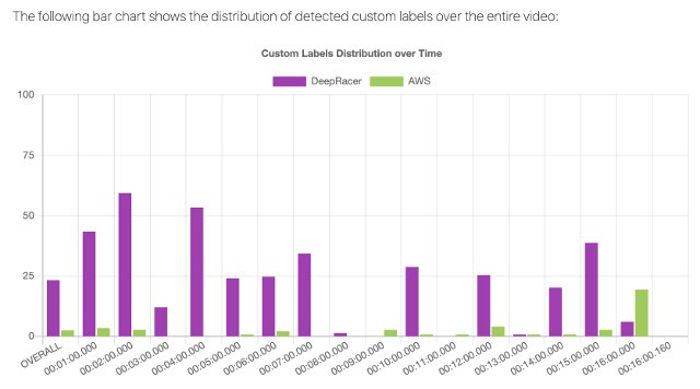
When our model is trained, Amazon Rekognition Custom Labels provides an inference endpoint. We can then upload and analyze images or video files using the inference endpoint. The web user interface presents a bar chart that shows the distribution of detected custom labels per minute in the analyzed video.
Architecture overview
The solution uses the serverless architecture. The following architectural diagram illustrates an overview of the solution.

The solution is composed of two AWS Step Functions state machines:
- Training – Manages extracting image frames from uploaded videos, creating and waiting on a Ground Truth labeling job, and creating and training an Amazon Rekognition Custom Labels model. You can then use the model to run brand logo detection analysis.
- Analysis – Handles analyzing video or image files. It manages extracting image frames from the video files, starting the custom label model, running the inference, and shutting down the custom label model.
The solution provides a built-in mechanism to manage your custom label model runtime to ensure the model is shut down to keep your cost at a minimum.
The web application communicates with the backend state machines using an Amazon API Gateway RESTful endpoint. The endpoint is protected with a valid AWS Identity and Access Management (IAM) credential. The authentication to the web application is done through an Amazon Cognito user pool, where an authenticated user is issued a secure, time-bounded, temporary credential that can then be used to access “scoped” resources such as uploading video and image files to an Amazon Simple Storage Service (Amazon S3) bucket, invoking the API Gateway RESTful API endpoint to create a new training project, or running inference with the Amazon Rekognition Custom Labels model you trained and built. We use Amazon CloudFront to host the static contents residing on an S3 bucket (web), which is protected through OAID.
Prerequisites
For this walkthrough, you should have an AWS account with appropriate IAM permissions to launch the provided AWS CloudFormation template.
Deploying the solution
You can deploy the solution using a CloudFormation template with AWS Lambda-backed custom resources. To deploy the solution, use one of the following CloudFormation templates and follows the instructions:
| AWS Region | CloudFormation Template URL |
| US East (N. Virginia) | |
| US East (Ohio) | |
| US West (Oregon) | |
| EU (Ireland) |
- Sign in to the AWS Management Console with your IAM user name and password.
- On the Create stack page, choose Next.

- On the Specify stack details page, for FFmpeg Component, choose AGREE AND INSTALL.
- For Email, enter a valid email address to use for administrative purposes.
- For Price Class, choose Use Only U.S., Canada and Europe [PriceClass_100].
- Choose Next.

- On the Review stack page, under Capabilities, select both check boxes.
- Choose Create stack.

The stack creation takes roughly 25 minutes to complete; we’re using Amazon CodeBuild to dynamically build the FFmpeg component, and Amazon CloudFront distribution takes about 15 minutes to propagate to the edge locations.
After the stack is created, you should receive an invitation email from no-reply@verificationmail.com. The email contains a CloudFront URL link to access the demo portal, your login username, and a temporary password.

Choose the URL link to open the web portal with Mozilla Firefox or Google Chrome. After you enter your user name and temporary credentials, you’re prompted to create a new password.
Solution walkthrough
In this section, we walk you through the following high-level steps:
- Setting up a labeling team.
- Creating and training your model.
- Completing a video object detection labeling job.
Setting up a labeling team
The first time you log in to the web portal, you’re prompted to create your labeling workforce. The labeling workforce defines members of your labelers who are given labeling tasks to work on when you start a new training project. Choose Yes to configure your labeling team members.

You can also navigate to the Labeling Team tab to manage members from your labeling team at any time.
Follow the instructions to add an email and choose Confirm and add members. See the following animation to walk you through the steps.

The newly added member receives two email notifications. The first email contains the credential for the labeler to access the labeling portal. It’s important to note that the labeler is only given access to consume a labeling job created by Ground Truth. They don’t have access to any AWS resources other than working on the labeling job.

A second email “AWS Notification – Subscription Confirmation” contains instructions to confirm your subscription to an Amazon Simple Notification Service (Amazon SNS) topic so the labeler gets notified whenever a new labeling task is ready to consume.

Creating and training your first model
Let’s start to train our first model to identify logos for AWS and AWS DeepRacer. For this post, we use the video file AWS DeepRacer TV – Ep 1 Amsterdam.
- On the navigation menu, choose Training.
- Choose Option 1 to train a model to identify the logos with bounding boxes.
- For Project name, enter
DemoProject. - Choose Add label.
- Add the labels
AWSandDeepRacer. - Drag and drop a video file to the drop area.
You can drop multiple video or JPEG or PNG image files.
- Choose Create project.
The following GIF animation illustrates the process.

At this point, a labeling job is soon created by Ground Truth and the labeler receives an email notification when the job is ready to consume.
Completing the video object detection labeling job
Ground Truth recently launched a new set of pre-built templates that help label video files. For our post, we use the video object detection task template. For more information, see New – Label Videos with Amazon SageMaker Ground Truth.
The training workflow is currently paused, waiting for the labelers to work on the labeling job.
- After the labeler receives an email notification that a job is ready for them, they can log in to the labeling portal and start the job by choosing Start working.
- For Label category, choose a label.
- Draw bounding boxes around the AWS or AWS DeepRacer logos.
You can use the Predict next button to predict the bounding box in subsequent frames.
The following GIF animation demonstrates the labeling flow.

After the labeler completes the job, the backend training workflow resumes and collects the labeled images from the Ground Truth labeling job and starts the model training by creating an Amazon Rekognition Custom Labels project. The time to train a model varies from an hour to a few hours depending on the complexity of the objects (labels) and the size of your training dataset. Amazon Rekognition Custom Labels automatically splits the dataset 80/20 to create the training dataset and test dataset, respectively.
Running inference to detect brand logos
After the model is trained, let’s upload a video file and run predictions with the model we trained.
- On the navigation menu, choose Analysis.
- Choose Start new analysis.
- Specify the following:
- Project name – The project we created in Amazon Rekognition Custom Labels.
- Project version – The specific version of the trained model.
- Inference units – Your desired inference units, so you can dial up or dial down the inference endpoint. For example, if you require higher transactions per second (TPS), use a larger number of inference endpoint.
- Drop and drop image files (JPEG, PNG) or video files (MP4, MOV) to the drop area.
- When the upload is complete, choose Done and wait for the analysis process to finish.
The analysis workflow starts and waits for the trained Amazon Rekognition Custom Labels model, runs the inference frame by frame, and shuts the model down when it’s no longer in use.
The following GIF animation demonstrates the analysis flow.

Viewing prediction results
The solution provides an overall statistic of the detected brands distributed across the video. The following screenshot shows that the AWS DeepRacer logo is detected about 25% overall and is detected approximately 60% in the 00:01:00–00:02:00 timespan. In contrast, the AWS logo is detected at a much lower rate. For this post, we only used one video to train the model, which had relatively few AWS logos. We can improve the accuracy by retraining the model with more video files.
You can expand the shot element view to see how the brand logos are detected frame by frame.

If you choose a frame to view, it shows the logo with a confidence score. The images that are grayed out are the ones that don’t detect any logo. The following image shows that the AWS DeepRacer logo is detected at frame #10237 with a confidence score of 82%.

Another image shows that the AWS logo is detected with a confidence score of 60%.

Cleaning up
To delete the demo solution, simply delete the CloudFormation stack that you deployed earlier. However, deleting the CloudFormation stack doesn’t remove the following resources, which you must clean up manually to avoid potential recurring costs:
- S3 buckets (web, source, and logs)
- Amazon Rekognition Custom Labels project (trained model)
Conclusion
This post demonstrated how to use Amazon Rekognition Custom Labels to detect brand logos in images and videos. No ML expertise is required to build your own model. The ease of use and intuitive setup of Amazon Rekognition Custom Labels allows you to bring your own dataset, label it into separate folders, and launch the Amazon Rekognition Custom Labels training and validation. We created the required infrastructure, demonstrated installing and running the UI, and discussed the security and cost of the infrastructure.
In the second post in this series, we deep dive into data labeling from a video file using Ground Truth to prepare the data for the training phase. We also explain the technical details of how we use Amazon Rekognition Custom Labels to train the model. In the third post in this series, we dive into the inference phase and show you the reach set of statistics for your brand visibility in a given video file.
For more information about the code sample in this post, see the GitHub repo.
About the Authors
 Ken Shek is a Global Vertical Solutions Architect, Media and Entertainment in EMEA region. He helps media customers to designs, develops, and deploys workloads onto AWS Cloud using the AWS Cloud best practice. Ken graduated from University of California, Berkeley and received his master degree in Computer Science at Northwestern Polytechnical University.
 Amit Mukherjee is a Sr. Partner Solutions Architect with a focus on Data Analytics and AI/ML. He works with AWS partners and customers to provide them with architectural guidance for building highly secure scalable data analytics platform and adopt machine learning at a large scale.
 Sameer Goel is a Solutions Architect in Seattle, who drives customer’s success by building prototypes on cutting-edge initiatives. Prior to joining AWS, Sameer graduated with Master’s Degree from NEU Boston, with Data Science concentration. He enjoys building and experimenting creative projects and applications.
Model serving made easier with Deep Java Library and AWS Lambda
Developing and deploying a deep learning model involves many steps: gathering and cleansing data, designing the model, fine-tuning model parameters, evaluating the results, and going through it again until a desirable result is achieved. Then comes the final step: deploying the model.
AWS Lambda is one of the most cost effective service that lets you run code without provisioning or managing servers. It offers many advantages when working with serverless infrastructure. When you break down the logic of your deep learning service into a single Lambda function for a single request, things become much simpler and easy to scale. You can forget all about the resource handling needed for the parallel requests coming into your model. If your usage is sparse and tolerable to a higher latency, Lambda is a great choice among various solutions.
Now, let’s say you’ve decided to use Lambda to deploy your model. You go through the process, but it becomes confusing or complex with the various setup steps to run your models. Namely, you face issues with the Lambda size limits and managing the model dependencies within.
Deep Java Library (DJL) is a deep learning framework designed to make your life easier. DJL uses various deep learning backends (such as Apache MXNet, PyTorch, and TensorFlow) for your use case and is easy to set up and integrate within your Java application! Thanks to its excellent dependency management design, DJL makes it extremely simple to create a project that you can deploy on Lambda. DJL helps alleviate some of the problems we mentioned by downloading the prepackaged framework dependencies so you don’t have to package them yourself, and loads your models from a specified location such as Amazon Simple Storage Service (Amazon S3) so you don’t need to figure out how to push your models to Lambda.
This post covers how to get your models running on Lambda with DJL in 5 minutes.
About DJL
Deep Java Library (DJL) is a Deep Learning Framework written in Java, supporting both training and inference. DJL is built on top of modern deep learning engines (such as TenserFlow, PyTorch, and MXNet). You can easily use DJL to train your model or deploy your favorite models from a variety of engines without any additional conversion. It contains a powerful model zoo design that allows you to manage trained models and load them in a single line. The built-in model zoo currently supports more than 70 pre-trained and ready-to-use models from GluonCV, HuggingFace, TorchHub, and Keras.
Prerequisites
You need the following items to proceed:
- An AWS account with access to Lambda
- The AWS Command Line Interface (AWS CLI) installed on your system and configured with your credentials and Region
- A Java environment set up on your system
In this post, we follow along with the steps from the following GitHub repo.
Building and deploying on AWS
First we need to ensure we’re in the correct code directory. We need to create the an S3 bucket for storage, an AWS CloudFormation stack, and the Lambda function with the following code:
cd lambda-model-serving
./gradlew deploy
This creates the following:
- An S3 bucket with the name stored in bucket-name.txt
- A CloudFormation stack named
djl-lambdaand a template file named out.yml - A Lambda function named
DJL-Lambda
Now we have our model deployed on a serverless API. The next section invokes the Lambda function.
Invoking the Lambda function
We can invoke the Lambda function with the following code:
aws lambda invoke --function-name DJL-Lambda --payload '{"inputImageUrl":"https://djl-ai.s3.amazonaws.com/resources/images/kitten.jpg"}' build/output.jsonThe output is stored into build/output.json:
cat build/output.json
[
  {
    "className": "n02123045 tabby, tabby cat",
    "probability": 0.48384541273117065
  },
  {
    "className": "n02123159 tiger cat",
    "probability": 0.20599405467510223
  },
  {
    "className": "n02124075 Egyptian cat",
    "probability": 0.18810519576072693
  },
  {
    "className": "n02123394 Persian cat",
    "probability": 0.06411759555339813
  },
  {
    "className": "n02127052 lynx, catamount",
    "probability": 0.01021555159240961
  }
]
Cleaning up
Use the cleanup scripts to clean up the resources and tear down the services created in your AWS account:
./cleanup.shCost analysis
What happens if we try to set this up on an Amazon Elastic Compute Cloud (Amazon EC2) instance and compare the cost to Lambda? EC2 instances need to continuously run for it to receive requests at any time. This means that you’re paying for that additional time when it’s not in use. If we use a cheap t3.micro instance with 2 vCPUs and 1 GB of memory (knowing that some of this memory is used by the operating system and for other tasks), the cost comes out to $7.48 a month or about 1.6 million requests to Lambda. When using a more powerful instance such as t3.small with 2 vCPUs and 4 GB of memory, the cost comes out to $29.95 a month or about 2.57 million requests to Lambda.
There are pros and cons with using either Lambda or Amazon EC2 for hosting, and it comes down to requirements and cost. Lambda is the ideal choice if your requirements allow for sparse usage and higher latency due to the cold startup of Lambda (5-second startup) when it isn’t used frequently, but it’s cheaper than Amazon EC2 if you aren’t using it much, and the first call can be slow. Subsequent requests become faster, but if Lambda sits idly for 30–45 minutes, it goes back to cold-start mode.
Amazon EC2, on the other hand, is better if you require low latency calls all the time or are making more requests than what it costs in Lambda (shown in the following chart).

Minimal package size
DJL automatically downloads the deep learning framework at runtime, allowing for a smaller package size. We use the following dependency:
runtimeOnly "ai.djl.mxnet:mxnet-native-auto:1.7.0-backport"This auto-detection dependency results in a .zip file less than 3 MB. The downloaded MXNet native library file is stored in a /tmp folder that takes up about 155 MB of space. We can further reduce this to 50 MB if we use a custom build of MXNet without MKL support.
The MXNet native library is stored in an S3 bucket, and the framework download latency is negligible when compared to the Lambda startup time.
Model loading
The DJL model zoo offers many easy options to deploy models:
- Bundling the model in a .zip file
- Loading models from a custom model zoo
- Loading models from an S3 bucket (supports Amazon SageMaker trained model .tar.gz format)
We use the MXNet model zoo to load the model. By default, because we didn’t specify any model, it uses the resnet-18 model, but you can change this by passing in an artifactId parameter in the request:
aws lambda invoke --function-name DJL-Lambda --payload '{"artifactId": "squeezenet", "inputImageUrl":"https://djl-ai.s3.amazonaws.com/resources/images/kitten.jpg"}' build/output.jsonLimitations
There are certain limitations when using serverless APIs, specifically in AWS Lambda:
- GPU instances are not yet available, as of this writing
- Lambda has a 512 MB limit for the
/tmpfolder - If the endpoint isn’t frequently used, cold startup can be slow
As mentioned earlier, this way of hosting your models on Lambda is ideal when requests are sparse and the requirement allows for higher latency calls due to the Lambda cold startup. If your requirements require low latency for all requests, we recommend using AWS Elastic Beanstalk with EC2 instances.
Conclusion
In this post, we demonstrated how to easily launch serverless APIs using DJL. To do so, we just need to run the gradle deployment command, which creates the S3 bucket, CloudFormation stack, and Lambda function. This creates an endpoint to accept parameters to run your own deep learning models.
Deploying your models with DJL on Lambda is a great and cost-effective method if Lambda has sparse usage and allows for high latency, due to its cold startup nature. Using DJL allows your team to focus more on designing, building, and improving your ML models, while keeping costs low and keeping the deployment process easy and scalable.
For more information on DJL and its other features, see Deep Java Library.
Follow our GitHub repo, demo repository, Slack channel, and Twitter for more documentation and examples of DJL!
About the Author
Frank Liu is a Software Engineer for AWS Deep Learning. He focuses on building innovative deep learning tools for software engineers and scientists. In his spare time, he enjoys hiking with friends and family.
Learning new language-understanding tasks from just a few examples
New approach to few-shot learning improves on state of the art by combining prototypical networks with data augmentation.Read More
Removing Spurious Feature can Hurt Accuracy and Affect Groups Disproportionately
Introduction
Machine learning models are susceptible to learning irrelevant patterns.
In other words, they rely on some spurious features that we humans know
to avoid. For example, assume that you are training a model to predict
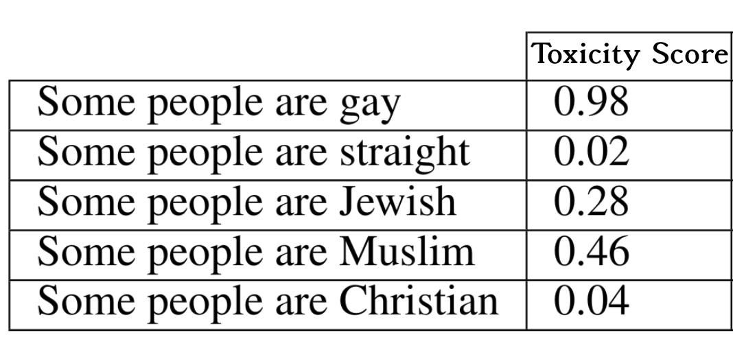
whether a comment is toxic on social media platforms. You would expect
your model to predict the same score for similar sentences with
different identity terms. For example, “some people are Muslim” and
“some people are Christian” should have the same toxicity score.
However, as shown in 1, training a convolutional
neural net leads to a model which assigns different toxicity scores to
the same sentences with different identity terms. Reliance on spurious
features is prevalent among many other machine learning models. For
instance, 2 shows that state of the art models in object
recognition like Resnet-50 3 rely heavily on background, so
changing the background can also change their predictions .
(Left) Machine learning models assign different toxicity scores to the
same sentences with different identity terms.
(Right) Machine learning models make different predictions on the same
object against different backgrounds.
Machine learning models rely on spurious features such as background in an image or identity terms in a comment. Reliance on spurious features conflicts with fairness and robustness goals.
Of course, we do not want our model to rely on such spurious features
due to fairness as well as robustness concerns. For example, a model’s
prediction should remain the same for different identity terms
(fairness); similarly its prediction should remain the same with
different backgrounds (robustness). The first instinct to remedy this
situation would be to try to remove such spurious features, for example,
by masking the identity terms in the comments or by removing the
backgrounds from the images. However, removing spurious features can
lead to drops in accuracy at test time 45. In this
blog post, we explore the causes of such drops in accuracy.
There are two natural explanations for accuracy drops:
- Core (non-spurious) features can be noisy or not expressive enough
so that even an optimal model has to use spurious features to
achieve the best accuracy
678. - Removing spurious features can corrupt the core features
910.
One valid question to ask is whether removing spurious features leads to
a drop in accuracy even in the absence of these two reasons. We answer
this question affirmatively in our recently published work in ACM Conference on Fairness, Accountability, and Transparency (ACM FAccT) 11. Here, we explain our results.
Removing spurious features can lead to drop in accuracy even when spurious features are removed properly and core features exactly determine the target!


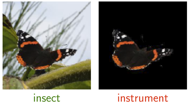
(Left) When core features are not representative (blurred image), the
spurious feature (the background) provides extra information to identify
the object. (Right) Removing spurious features (gender
information) in the sport prediction task has corrupted other core
features (the weights and the bar).
Before delving into our result, we note that understanding the reasons
behind the accuracy drop is crucial for mitigating such drops. Focusing
on the wrong mitigation method fails to address the accuracy drop.
Before trying to mitigate the accuracy drop resulting from the removal of the spurious features, we must understand the reasons for the drop.
| Previous work | Previous work | This work | |
|---|---|---|---|
 |
 |
 |
|
| Removing spurious features causes drops in accuracy because… | core features are noisy and not sufficiently expressive. | spurious features are not removed properly and thus corrupt core features. | a lack of training data causes spurious connections between some features and the target. |
| We can mitigate such drops by… | focusing on collecting more expressive features (e.g., high-resolution images) | focusing on more accurate methods for removing spurious features. | focusing on collecting more diverse training data. We show how to leverage unlabeled data to achieve such diversity. |
This work in a nutshell:
- We study overparameterized models that fit training data perfectly.
- We compare the “core model” that only uses core features (non-spurious) with the “full model” that uses both core features and spurious features.
- Using the spurious feature, the full model can fit training data with a smaller norm.
- In the overparameterized regime, since the number of training examples is less than the number of features, there are some directions of data variation that are not observed in the training data (unseen directions).
- Though both models fit the training data perfectly, they have different “assumptions’’ for the unseen directions. This difference can lead to
- Drop in accuracy
- Affecting different test distributions (we also call them groups) disproportionately (increasing accuracy in some while decreasing accuracy in others).

Noiseless Linear Regression
Over the last few years, researchers have observed some surprising
phenomena about deep networks that conflict with classical machine
learning. For example, training models to zero training loss leads to
better generalization instead of overfitting 12. A line
of work 1314 found that these unintuitive
results happen even for simple models such as linear regression if the
number of features are greater than the number of training data, known
as the overparameterized regime.
Accuracy drops due to the removal of spurious features is also
unintuitive. Classical machine learning tells us that removing spurious
features should decrease generalization error (since these features are,
by definition, irrelevant for the task). Analogous to the mentioned
work, we will explain this unintuitive result in overparameterized
linear regression as well.
Accuracy drop due to removal of the spurious feature can be explained in overparameterized linear regression.
Let’s first formalize the noiseless linear regression setup. Recall
that we are going to study a setup in which the target is completely
determined by the core features, and the spurious feature is a single
feature that can be removed perfectly without affecting predictive
performance. Formally, we assume there are (d) core features
(z in mathbb{R}^d) that determine the target (y in
mathbb{R}) perfectly, i.e., ( y = {theta^star}^top z).
In addition, we assume there is a single spurious feature (s) that
can also be determined by the core features (s =
{beta^star}^top z). Note that the spurious feature can have
information about features that determine the target or it can be
completely unrelated to the target (i.e., for all (i),
(beta^star_i theta^star_i=0)).
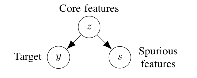
We consider a setup where target ((y)) is a deterministic function
of core features ((z)). In addition, there is a spurious feature
((s)) that can also be determined by the core feature. We compare
two models, the core model that only uses (z) to predict (y) and the full model which uses both (z) and (s) to predict
(y).
We consider two models:
- Core model that only uses the core features (z) to predict the
target (y), and it is parametrized by
({theta^text{-s}}). For a data point with core features
(z), its prediction is (hat y =
{theta^text{-s}}^top z). - Full model that uses the core features (z) and also uses the
spurious feature (s), and it is parametrized by
({theta^text{+s}}), and (w), For a data point with
core feature (z) and a spurious feature (s), its
prediction is (hat y = {theta^text{+s}}^top z + ws).
In this setup, the mentioned two reasons that naturally can cause
accuracy drop after removing the spurious feature (depicted in the table
above) do not exist.
- The spurious feature (s) adds no information about the target
(y) beyond what already exists in the core features
(z) (reason 1), - Removing (s) does not corrupt (z) (reason 2).
Motivated by recent work in deep learning, which speculates that
gradient descent converges to the minimum-norm solution that fits
training data perfectly 15, we consider the
minimum-norm solution.
- Training data: We assume we have (n < d) triples of
((z_i, s_i, y_i)) - Test data: We assume core features in the test data are from a
distribution with covariance matrix (Sigma =
mathbb{E}[zz^top]) (we use group and test data distribution
exchangeably).
In this simple setting, one might conjecture that removing the spurious
feature should only help accuracy. However, we show that this is not
always the case. We exactly characterize the test distributions that are
negatively affected by removing spurious features, as well as the ones
that are positively affected by it.
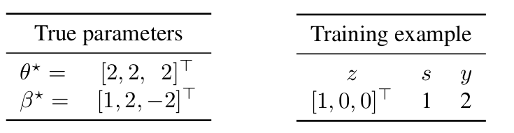
Example
Let’s first look at a simple example with only one training data and
three core features ((z_1, z_2) and (z_3)). Let the true
parameters (theta^star =[2,2,2]^top) which results in
(y=2), and let the spurious feature parameter ({beta^star}
= [1,2,-2]^top) which results in (s=1).
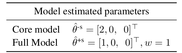
First, note that the smallest L2-norm vector that can fit the training
data for the core model is ({theta^text{-s}}=[2,0,0]). On
the other hand, in the presence of the spurious feature, the full model
can fit the training data perfectly with a smaller norm by assigning
weight (1) for the feature (s)
((|{theta^text{-s}}|_2^2 = 4) while
(|{theta^text{+s}}|_2^2 + w^2 = 2 < 4)).
Generally, in the overparameterized regime, since the number of training
examples is less than the number of features, there are some directions
of data variation that are not observed in the training data. In this
example, we do not observe any information about the second and third
features. The core model assigns weight (0) to the unseen
directions (weight (0) for the second and third features in this
example). However, the non-zero weight for the spurious feature leads to
a different assumption for the unseen directions. In particular, the
full model does not assign weight (0) to the unseen directions.
Indeed, by substituting (s) with ({beta^star}^top
z), we can view the full model as not using (s) but
implicitly assigning weight (beta^star_2=2) to the second
feature and (beta^star_3=-2) to the third feature (unseen
directions at training).
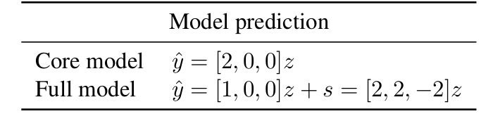
Let’s now look at different examples and the prediction of these two
models:
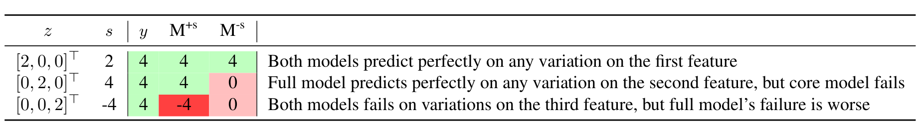
In this example, removing (s) reduces the error for a test
distribution with high deviations from zero on the second feature,
whereas removing (s) increases the error for a test distribution
with high deviations from zero on the third feature.
Main result
As we saw in the previous example, by using the spurious feature, the
full model incorporates ({beta^star}) into its estimate. The
true target parameter ((theta^star)) and the true spurious
feature parameters (({beta^star})) agree on some of the
unseen directions and do not agree on the others. Thus, depending on
which unseen directions are weighted heavily in the test time, removing
(s) can increase or decrease the error.
More formally, the weight assigned to the spurious feature is
proportional to the projection of (theta^star) on
({beta^star}) on the seen directions. If this number is close
to the projection of (theta^star) on ({beta^star})
on the unseen directions (in comparison to 0), removing (s)
increases the error, and it decreases the error otherwise. Note that
since we are assuming noiseless linear regression and choose models that
fit training data, the model predicts perfectly in the seen directions
and only variations in unseen directions contribute to the error.
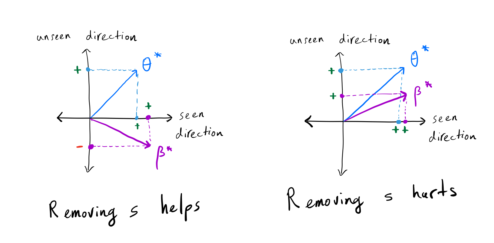
(Left) The projection of (theta^star) on
(beta^star) is positive in the seen direction, but it is
negative in the unseen direction; thus, removing (s) decreases the
error. (Right) The projection of (theta^star) on
(beta^star) is similar in both seen and unseen directions;
thus, removing (s) increases the error.
Drop in accuracy in test time depends on the relationship between the true target parameter ((theta^star)) and the true spurious feature parameters (({beta^star})) in the seen directions and unseen direction.
Let’s now formalize the conditions under which removing the spurious
feature ((s)) increases the error. Let (Pi =
Z(ZZ^top)^{-1}Z) denote the column space of training data (seen
directions), thus (I-Pi) denotes the null space of training data
(unseen direction). The below equation determines when removing the
spurious feature decreases the error.
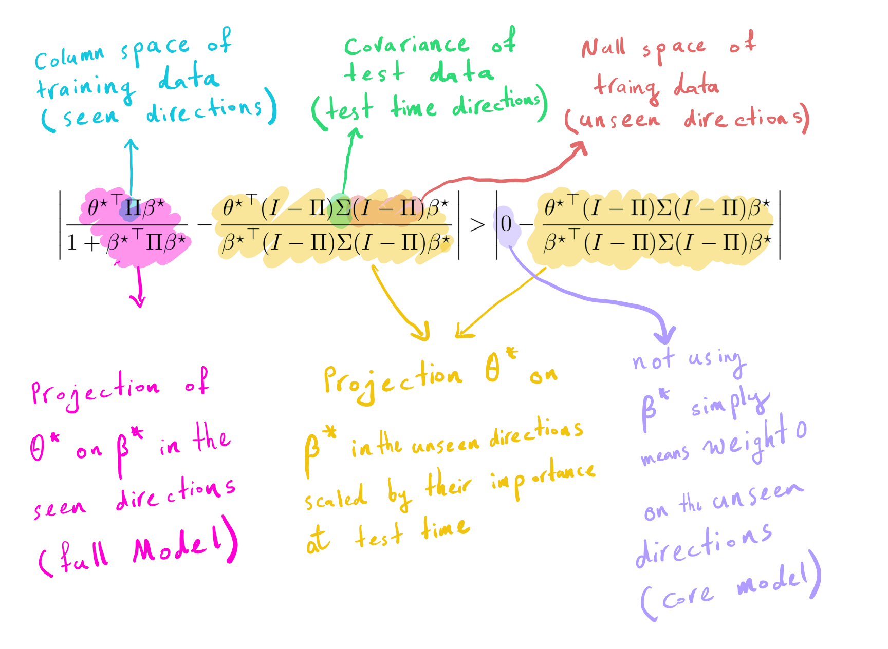
The left side is the difference between the projection of (theta^star) on (beta^star) in the seen direction
with their projection in the unseen direction scaled by test time
covariance. The right side is the difference between 0 (i.e., not using
spurious features) and the projection of (theta^star) on
(beta^star) in the unseen direction scaled by test time
covariance. Removing (s) helps if the left side is greater than
the right side.
Experiments
While the theory applies only to linear models, we now show that in
non-linear models trained on real-world datasets, removing a spurious
feature reduces the accuracy and affects groups disproportionately.
Datasets. We are going to study the CelebA dataset 16 which
contains photos of celebrities along with 40 different attributes.
footnote{See our paper for the results on the
comment-toxicity-detection and MNIST datasets} We choose wearing
lipstick (indicating if a celebrity is wearing lipstick) as the target
and wearing earrings (indicating if a celebrity is wearing earrings) as
the spurious feature.
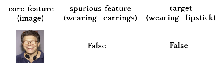
Note that although wearing earrings is correlated with wearing lipstick,
we expect our model to not change its prediction if we tell the model
the person is wearing earrings.
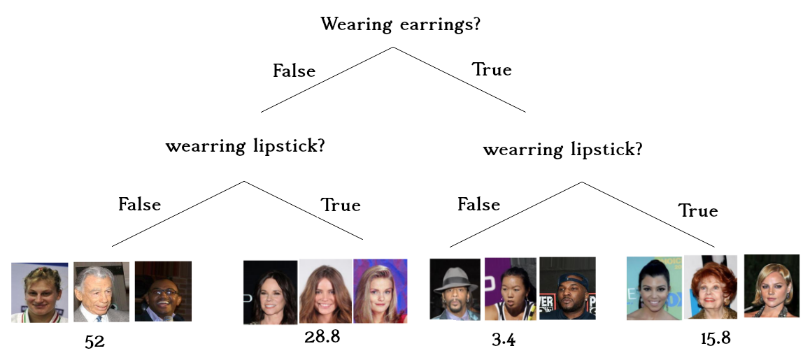
In the CelebA dataset wearing earrings is correlated with wearing
lipstick. In this dataset, if a celebrity wears earrings, it is almost
five times more likely that they will wear lipstick than not wearing
lipstick. Similarly, if a celebrity does not wear earrings, it is
almost two times more likely for them not to wear lipstick than wearing
lipstick.
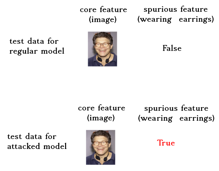
Setup. We train a two-layer neural network with 128 hidden units. We
flatten the picture and concatenate the binary variable of wearing
earrings to it (we tuned a multiplier for it). We also want to know how
much each model relies on the spurious feature. In other words, we want
to know how much the model prediction changes as we change the wearing
earrings variable. We call this attacking the model (i.e, swapping the
value of the binary feature of wearing earrings). We run each experiment
50 times and report the average.
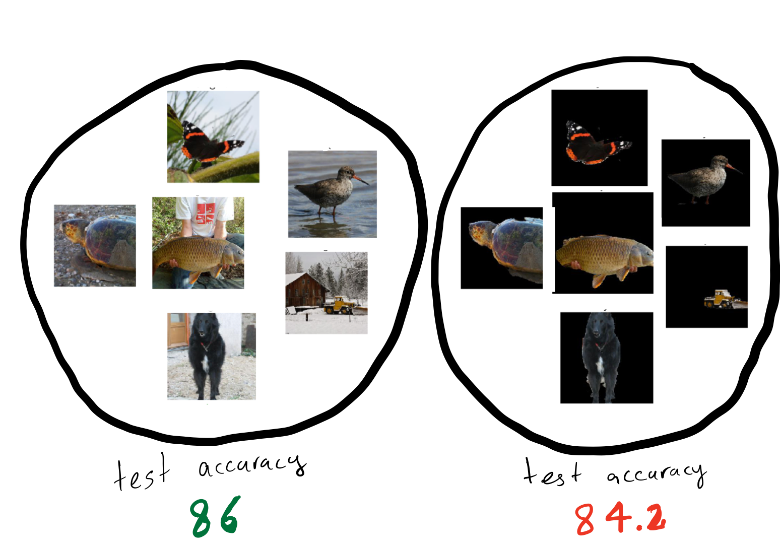
Results. The below diagram shows the accuracy of different models, and
their accuracies when they are attacked. Note that, because our attack
focuses on the spurious feature, the core model’s accuracy will remain
the same.
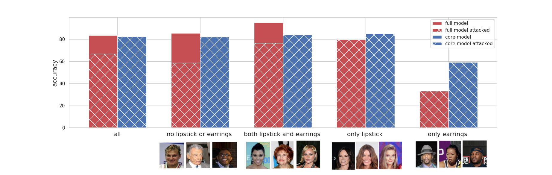
Removal of the wearing lipstick decreases the overall accuracy. The
decrease in accuracy is not monotonic among different groups. The
accuracy has decreased in the group where people are not wearing
lipstick or earrings and in the group that they both have lipstick and
earrings. On the other hand, accuracy increases for the group that only
wears one of them.
Let’s break down the diagram and analyze each section.
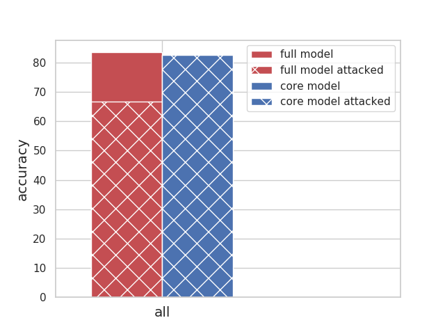 |
All celebrities together: have a reasonable accuracy of 82% The overall accuracy drops 1% when we remove the spurious feature (core model accuracy). The full model relies on the spurious feature a lot, thus attacking the full model leads to a ~ 17% drop in overall accuracy. |
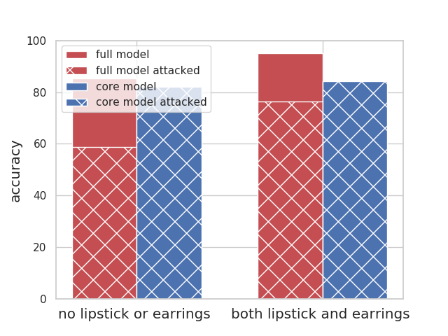 |
The celebrities who follow the stereotype (people who do not have earrings or lipstick, and people who wear both) have a good accuracy overall (both above 85%); The accuracy of both groups drop as we remove the wearing earrings (i.e., core model accuracy). Using the spurious feature helps their accuracy, thus attacking the full model leads to a ~30% drop in their accuracy. |
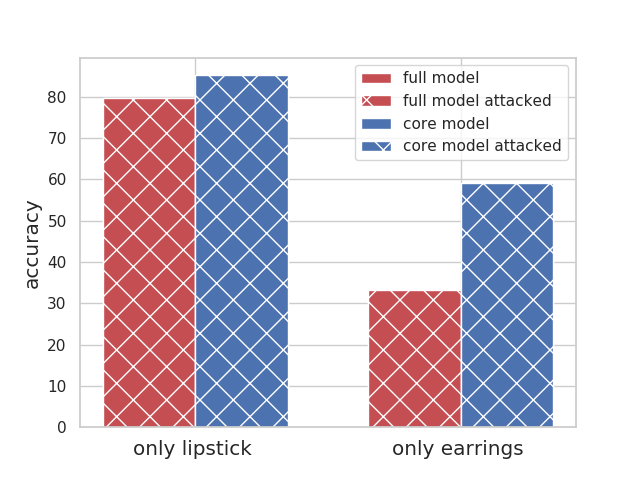 |
The celebrities who do not follow the stereotypes have a very low accuracy; this is especially worse for people who only wear earrings (33% accuracy in comparison to the average of 85%). Removing the wearing earring increases their accuracy substantially. Using the spurious feature does not help their accuracy, thus attacking the full model does not change accuracy for these groups. |
In non-linear models trained on real-world datasets, removing a spurious feature reduces the accuracy and affects groups disproportionately.
Q&A (Other results):
I know about my problem setting, and I am certain that disjoint features
determine the target and the spurious feature (i.e., for all (i),
(theta^star_ibeta^star_i=0)). Can I be sure that my
model will not rely on the spurious feature, and removing the spurious
feature definitely reduces the error? No! Actually, for any
(theta^star) and ({beta^star}), we can construct a
training set and two test sets with (theta^star) and
({beta^star}) as the true parameters and the spurious feature
parameter, such that removing the spurious feature reduces the error in
one but increases the error in the other one (see Corollary 1 in our
paper).
I am collecting a balanced dataset such that the spurious feature and
the target are completely independent (i.e., (p[y,s]= p[y]p[s])).
Can I be sure that my model will not rely on the spurious feature, and
removing the spurious feature definitely reduces the error?
No! for any
(S in mathbb{R}^n) and (Y in mathbb{R}^n), we can
generate a training set and two test sets with (S) and (Y)
as their spurious feature and targets, respectively, such that removing
the spurious feature reduces the error in one but increases the error in
the other (see Corollary 2 in our paper).
What happens when we have many spurious features? Good question! Let’s
say (s_1) and (s_2) are two spurious features. We show
that:
- Removing (s_1) makes the model more sensitive against
(s_2), and - If a group has high error because of the new assumption about unseen
direction enforced by using (s_2), then it will have an even
higher error by removing (s_1).
(See Proposition 3 in our paper).
Is it possible to have the same model (a model with the same assumptions
on unseen directions as the full model) without relying on the spurious
feature (i.e., be robust against the spurious feature)? Yes! You can
recover the same model as the full model without relying on the spurious
feature via robust self-training and unlabeled data (See Proposition 4).
Conclusion
In this work, we first showed that overparameterized models are
incentivized to use spurious features in order to fit the training data
with a smaller norm. Then we demonstrated how removing these spurious
features altered the model’s assumption on unseen directions.
Theoretically and empirically, we showed that this change could hurt the
overall accuracy and affect groups disproportionately. We also proved
that robustness against spurious features (or error reduction by
removing the spurious features) cannot be guaranteed under any condition
of the target and spurious feature. Consequently, balanced datasets do
not guarantee a robust model and practitioners should consider other
features as well. Studying the effect of removing noisy spurious
features is an interesting future direction.
Acknowledgement
I would like to thank Percy Liang, Jacob Schreiber and Megha Srivastava for their useful comments. The images in the introduction are from 1718 1920.
-
Dixon, Lucas, et al. “Measuring and mitigating unintended bias in text classification.” Proceedings of the 2018 AAAI/ACM Conference on AI, Ethics, and Society. 2018. ↩
-
Xiao, Kai, et al. “Noise or signal: The role of image backgrounds in object recognition.” arXiv preprint arXiv:2006.09994 (2020). ↩
-
He, Kaiming, et al. “Deep residual learning for image recognition.” Proceedings of the IEEE conference on computer vision and pattern recognition. 2016. ↩
-
Zemel, Rich, et al. “Learning fair representations.” International Conference on Machine Learning. 2013. ↩
-
Wang, Tianlu, et al. “Balanced datasets are not enough: Estimating and mitigating gender bias in deep image representations.” Proceedings of the IEEE/CVF International Conference on Computer Vision. 2019. ↩
-
Khani, Fereshte, and Percy Liang. “Feature Noise Induces Loss Discrepancy Across Groups.” International Conference on Machine Learning. PMLR, 2020. ↩
-
Kleinberg, Jon, and Sendhil Mullainathan. “Simplicity creates inequity: implications for fairness, stereotypes, and interpretability.” Proceedings of the 2019 ACM Conference on Economics and Computation. 2019. ↩
-
photo from Torralba, Antonio. “Contextual priming for object detection.” International journal of computer vision 53.2 (2003): 169-191. ↩
-
Zhao, Han, and Geoff Gordon. “Inherent tradeoffs in learning fair representations.” Advances in neural information processing systems. 2019. ↩
-
photo from Wang, Tianlu, et al. “Balanced datasets are not enough: Estimating and mitigating gender bias in deep image representations.” Proceedings of the IEEE International Conference on Computer Vision. 2019. ↩
-
Khani, Fereshte, and Percy Liang. “Removing Spurious Features can Hurt Accuracy and Affect Groups Disproportionately.” arXiv preprint arXiv:2012.04104 (2020). ↩
-
Nakkiran, Preetum, et al. “Deep double descent: Where bigger models and more data hurt.” arXiv preprint arXiv:1912.02292 (2019). ↩
-
Hastie, T., Montanari, A., Rosset, S., & Tibshirani, R. J. (2019). Surprises in high-dimensional ridgeless least squares interpolation. arXiv preprint arXiv:1903.08560. ↩
-
Raghunathan, Aditi, et al. “Understanding and mitigating the tradeoff between robustness and accuracy.” arXiv preprint arXiv:2002.10716 (2020). ↩
-
Gunasekar, Suriya, et al. “Implicit regularization in matrix factorization.” 2018 Information Theory and Applications Workshop (ITA). IEEE, 2018. ↩
-
Liu, Ziwei, et al. “Deep learning face attributes in the wild.” Proceedings of the IEEE international conference on computer vision. 2015. ↩
-
Xiao, Kai, et al. “Noise or signal: The role of image backgrounds in object recognition.” arXiv preprint arXiv:2006.09994 (2020). ↩
-
Garg, Sahaj, et al. “Counterfactual fairness in text classification through robustness.” Proceedings of the 2019 AAAI/ACM Conference on AI, Ethics, and Society. 2019. ↩
-
photo from Torralba, Antonio. “Contextual priming for object detection.” International journal of computer vision 53.2 (2003): 169-191. ↩
-
photo from Wang, Tianlu, et al. “Balanced datasets are not enough: Estimating and mitigating gender bias in deep image representations.” Proceedings of the IEEE International Conference on Computer Vision. 2019. ↩
Accelerating rural connectivity research: How Facebook helps bring connectivity to hard-to-reach areas
All deployment site photos from Peru were taken by our partners at Mayu Telecomunicaciones are used here with permission. To request permission to use the photos, contact servicios@mayutel.com.
Facebook Connectivity’s mission is to enable better, broader global connectivity to bring more people online to a faster internet. We collaborate with others in the industry — including telecom operators, community leaders, technology developers, and researchers — in order to find solutions that are scalable and sustainable. One major research area of interest is rural connectivity, as many rural areas around the world still don’t have access to mobile connectivity and technology innovations are needed. An important element of rural connectivity is backhaul, the links that connect remote sites to the core network of the internet. Wireless backhaul using microwave radio provides low-cost, fast deployment in comparison with other options.
Today, the design of microwave backhaul relies on clear line-of-sight (LOS) requirements. Unfortunately, for rural areas, lack of LOS between settlements means that a repeater or reflector has to be built, which leads to cost constraints. In this project, we explore the use of diffraction, a physics phenomenon through which some wireless signal energy is bent into the geometric shadow of the obstacle. If diffraction can be predicted reliably, it could be used to design and build wireless backhaul links in challenging environments, reducing the need to build repeaters and making network design more efficient.
 Example physics-based signal propagation modeling result showing that some signal energy is diffracted into the shadow region
 Illustration of how diffractive NLOS wireless links can reduce the need to build repeaters
To address this challenge, Facebook Connectivity developed a research partnership with university and industry partners. We recognized that we need field data that can be used to validate and calibrate signal prediction algorithms, improved network design methodologies, and an assessment of real-world cost-coverage impact. To facilitate knowledge sharing and collaboration, Facebook Connectivity organized a number of meetings, including a workshop in 2019. In this workshop, Omar Tupayachi Calderon (CEO of Mayu Telecomunicaciones, a rural mobile infrastructure operator in Peru) shared that “Peru has an incredible diversity of challenges, and 60,000 rural settlements still do not have broadband connectivity. We need your help.”
Bringing rural connectivity to Peru
Universidad Politécnica de Madrid (UPM), The Ohio State University (OSU), Air Electronics, and Plexus Controls developed instruments to measure signal propagation over difficult terrain and conducted systematic experiments in southern Ohio, in areas near Madrid, Spain, and in southern Ontario, Canada. University of Michigan, George Mason University, OSU, and MIT developed propagation models, resulting in a number of publications and open source software.


Experimental data and setups used by OSU and UPM (click to enlarge)
The complete solution set that Facebook developed included an end-to-end workflow for link design, network planning, and site deployment, which we are sharing as a white paper in the Telecom Infra Project Network as a Service Solution project group.


Rural Peru deployment pictures taken by Mayutel (click to enlarge)
Scaling the solution
To make the solution usable in as many parts of the world as possible, Facebook took several next steps:
First, we collaborated with OSU and George Mason University to make a MATLAB and Python version of the Irregular Terrain Model and Longley-Rice algorithm available as free, open source software.
Second, we broadened the collaboration to include Contract Telecommunications LTD — the makers of Pathloss, the most widely used microwave link planning software in the world — to implement the outputs of this project into their platform.
Third, we developed a field-grade drone-mounted measurement kit with Plexus Controls to enable experimentalists to gather field data economically, and for connectivity infrastructure developers to validate signal strength in the field prior to building their sites. Further, we developed a software for data visualization and basic processing. The drone and the software are designed to enable faster, simpler field experiments and validation than ever before.
Fourth, we are contributing our learnings to the Telecom Infra Project Network as a Service Solution Group.
Finally, we have expanded our partnership through collaborations with TeleworX, Internet para Todos (IpT) de Peru, and Mayu Telecomunicaciones (Mayutel). IpT de Peru is a major network operator that is significantly expanding broadband access in rural parts of the country. Founded in 2019, IpT has deployed hundreds of broadband sites in rural areas of Peru to date. IpT has successfully deployed dozens of NLOS links in their network, providing both end point and backbone transport connectivity. Mayutel works with the local communities in rural Peru to build the telecom sites, deploy 4G radio systems, and provide broadband connectivity for the first time to many of the community.
Learn more
As we look forward to bringing this solution to other parts of the world, please learn more about the technology behind this project through our publications:
- Diffractive NLOS Microwave Backhaul for Rural Connectivity
Julius Kusuma, Erik Boch, Philip Liddell (Facebook Connectivity) - Development of Measurement and Modeling Procedures of Diffractive near-LOS Wireless Links
José Manuel Riera, Santiago Pérez-Peña, Marta Castiella-Fernández, Pedro Velasco-de-la-Fuente, Mateo Burgos-García, Pedro Garcia-del-Pino, Luis Mendo (Universidad Politécnica de Madrid, Spain), Julius Kusuma, Erik Boch (Facebook Connectivity) - Gabor Frame-Based Sparsification and Radiation Boundary Conditions for Parabolic Wave Equations
Max Bright, Eric Michielssen (University of Michigan at Ann Arbor), Julius Kusuma (Facebook Connectivity) - Hybrid Parabolic Equation – Integral Equation Solvers for Analyzing Long Range Propagation Over Complex Terrain
Eric Michielssen, Max Bright (University of Michigan at Ann Arbor), Julius Kusuma (Facebook Connectivity) - Improving Rural Connectivity Coverage using Diffractive Non-Line of Sight (NLOS) Wireless Backhaul
Julius Kusuma, Erik Boch (Facebook Connectivity) - itmlogic: The Irregular Terrain Model by Longley and Rice
Edward J. Oughton (University of Oxford; University of Cambridge), Tom Russell (University of Oxford), Joel Johnson (The Ohio State University), Caglar Yardim (The Ohio State University), and Julius Kusuma (Facebook Connectivity)
To learn about NLOS in the Telecom Infra Project Network-as-a-Service Solutions project group, please see our recently published white paper on the subject. For more about the Telecom Infra Project, visit their website. You can also learn about other initiatives on the Facebook Connectivity website.
The post Accelerating rural connectivity research: How Facebook helps bring connectivity to hard-to-reach areas appeared first on Facebook Research.
Multi-account model deployment with Amazon SageMaker Pipelines
Amazon SageMaker Pipelines is the first purpose-built CI/CD service for machine learning (ML). It helps you build, automate, manage, and scale end-to-end ML workflows and apply DevOps best practices of CI/CD to ML (also known as MLOps).
Creating multiple accounts to organize all the resources of your organization is a good DevOps practice. A multi-account strategy is important not only to improve governance but also to increase security and control of the resources that support your organization’s business. This strategy allows many different teams inside your organization, to experiment, innovate, and integrate faster, while keeping the production environment safe and available for your customers.
Pipelines makes it easy to apply the same strategy to deploying ML models. Imagine a use case in which you have three different AWS accounts, one for each environment: data science, staging, and production. The data scientist has the freedom to run experiments and train and optimize different models any time in their own account. When a model is good enough to be deployed in production, the data scientist just needs to flip the model approval status to Approved. After that, an automated process deploys the model on the staging account. Here you can automate testing of the model with unit tests or integration tests or test the model manually. After a manual or automated approval, the model is deployed to the production account, which is a more tightly controlled environment used to serve inferences on real-world data. With Pipelines, you can implement a ready-to-use multi-account environment.
In this post, you learn how to use Pipelines to implement your own multi-account ML pipeline. First, you learn how to configure your environment and prepare it to use a predefined template as a SageMaker project for training and deploying a model in two different accounts: staging and production. Then, you see in detail how this custom template was created and how to create and customize templates for your own SageMaker projects.
Preparing the environment
In this section, you configure three different AWS accounts and use SageMaker Studio to create a project that integrates a CI/CD pipeline with the ML pipeline created by a data scientist. The following diagram shows the reference architecture of the environment that is created by the SageMaker custom project and how AWS Organizations integrates the different accounts.

The diagram contains three different accounts, managed by Organizations. Also, three different user roles (which may be the same person) operate this environment:
- ML engineer – Responsible for provisioning the SageMaker Studio project that creates the CI/CD pipeline, model registry, and other resources
- Data scientist – Responsible for creating the ML pipeline that ends with a trained model registered to the model group (also referred to as model package group)
- Approver – Responsible for testing the model deployed to the staging account and approving the production deployment
It’s possible to run a similar solution without Organizations, if you prefer (although not recommended). But you need to prepare the permissions and the trust relationship between your accounts manually and modify the template to remove the Organizations dependency. Also, if you’re an enterprise with multiple AWS accounts and teams, it’s highly recommended that you use AWS Control Tower for provisioning the accounts and Organizations. AWS Control Tower provides the easiest way to set up and govern a new and secure multi-account AWS environment. For this post, we only discuss implementing the solution with Organizations.
But before you move on, you need to complete the following steps, which are detailed in the next sections:
- Create an AWS account to be used by the data scientists (data science account).
- Create and configure a SageMaker Studio domain in the data science account.
- Create two additional accounts for production and staging.
- Create an organizational structure using Organizations, then invite and integrate the additional accounts.
- Configure the permissions required to run the pipelines and deploy models on external accounts.
- Import the SageMaker project template for deploying models in multiple accounts and make it available for SageMaker Studio.
Configuring SageMaker Studio in your account
Pipelines provides built-in support for MLOps templates to make it easy for you to use CI/CD for your ML projects. These MLOps templates are defined as Amazon CloudFormation templates and published via AWS Service Catalog. These are made available to data scientists via SageMaker Studio, an IDE for ML. To configure Studio in your account, complete the following steps:
- Prepare your SageMaker Studio domain.
- Enable SageMaker project templates and SageMaker JumpStart for this account and Studio users.
If you have an existing domain, you can simply edit the settings for the domain or individual users to enable this option. Enabling this option creates two different AWS Identity and Account Management (IAM) roles in your AWS account:
- AmazonSageMakerServiceCatalogProductsLaunchRole – Used by SageMaker to run the project templates and create the required infrastructure resources
- AmazonSageMakerServiceCatalogProductsUseRole – Used by the CI/CD pipeline to run a job and deploy the models on the target accounts
If you created your SageMaker Studio domain before re:Invent 2020, it’s recommended that you refresh your environment by saving all the work in progress. On the File menu, choose Shutdown, and confirm your choice.
- Create and prepare two other AWS accounts for staging and production, if you don’t have them yet.
Configuring Organizations
You need to add the data science account and the two additional accounts to a structure in Organizations. Organizations helps you to centrally manage and govern your environment as you grow and scale your AWS resources. It’s free and benefits your governance strategy.
Each account must be added to a different organizational unit (OU).
- On the Organizations console, create a structure of OUs like the following:
- Root
multi-account-deployment (OU)- 111111111111 (data science account—SageMaker Studio)
production(OU)- 222222222222 (AWS account)
staging(OU)- 333333333333 (AWS account)
After configuring the organization, each account owner receives an invite. The owners need to accept the invites, otherwise the accounts aren’t included in the organization.
- Now you need to enable trusted access with AWS organizations (“Enable all features” and “Enable trusted access in the StackSets”).
This process allows your data science account to provision resources in the target accounts. If you don’t do that, the deployment process fails. Also, this feature set is the preferred way to work with Organizations, and it includes consolidating billing features.
- Next, on the Organizations console, choose Organize accounts.
- Choose staging.
- Note down the OU ID.
- Repeat this process for the
productionOU.

Configuring the permissions
You need to create a SageMaker execution role in each additional account. These roles are assumed by AmazonSageMakerServiceCatalogProductsUseRole in the data science account to deploy the endpoints in the target accounts and test them.
- Sign in to the AWS Management Console with the staging account.
- Run the following CloudFormation template.
This template creates a new SageMaker role for you.
- Provide the following parameters:
- SageMakerRoleSuffix – A short string (maximum 10 lowercase with no spaces or alpha-numeric characters) that is added to the role name after the following prefix:
sagemaker-role-. The final role name issagemaker-role-<<sagemaker_role_suffix>>. - PipelineExecutionRoleArn – The ARN of the role from the data science account that assumes the SageMaker role you’re creating. To find the ARN, sign in to the console with the data science account. On the IAM console, choose Roles and search for
AmazonSageMakerServiceCatalogProductsUseRole. Choose this role and copy the ARN (arn:aws:iam::<<data_science_acccount_id>>:role/service-role/AmazonSageMakerServiceCatalogProductsUseRole).
- SageMakerRoleSuffix – A short string (maximum 10 lowercase with no spaces or alpha-numeric characters) that is added to the role name after the following prefix:
- After creating this role in the staging account, repeat this process for the production account.
In the data science account, you now configure the policy of the Amazon Simple Storage Service (Amazon S3) bucket used to store the trained model. For this post, we use the default SageMaker bucket of the current Region. It has the following name format: sagemaker-<<region>>-<<aws_account_id>>.
- On the Amazon S3 console, search for this bucket, providing the Region you’re using and the ID of the data science account.
If you don’t find it, create a new bucket following this name format.
- On the Permissions tab, add the following policy:
{
    "Version": "2012-10-17",
    "Statement": [
        {
            "Effect": "Allow",
            "Principal": {
                "AWS": [
                    "arn:aws:iam::<<staging_account_id>>:root",
                    "arn:aws:iam::<<production_account_id>>:root"
                ]
            },
            "Action": [
                "s3:GetObject",
                "s3:ListBucket"
            ],
            "Resource": [
                "arn:aws:s3:::sagemaker-<<region>>-<<aws_account_id>>",
                "arn:aws:s3:::sagemaker-<<region>>-<<aws_account_id>>/*"
            ]
        }
    ]
}
- Save your settings.
The target accounts now have permission to read the trained model during deployment.
The next step is to add new permissions to the roles AmazonSageMakerServiceCatalogProductsUseRole and AmazonSageMakerServiceCatalogProductsLaunchRole.
- In the data science account, on the IAM console, choose Roles.
- Find the
AmazonSageMakerServiceCatalogProductsUseRolerole and choose it. - Add a new policy and enter the following JSON code.
- Save your changes.
- Now, find the
AmazonSageMakerServiceCatalogProductsLaunchRolerole, choose it and add a new policy with the following content:{ "Version": "2012-10-17", "Statement": [ { "Sid": "VisualEditor0", "Effect": "Allow", "Action": "s3:GetObject", "Resource": "arn:aws:s3:::aws-ml-blog/artifacts/sagemaker-pipeline-blog-resources/*" } ] }
- Save your changes.
That’s it! Your environment is almost ready. You only need one more step and you can start training and deploying models in different accounts.
Importing the custom SageMaker Studio project template
In this step, you import your custom project template.
- Sign in to the console with the data science account.
- On the AWS Service Catalog console, under Administration, choose Portfolios.
- Choose Create a new portfolio.
- Name the portfolio
SageMaker Organization Templates. - Download the following template to your computer.
- Choose the new portfolio.
- Choose Upload a new product.
- For Product name¸ enter
Multi Account Deployment. - For Description, enter
Multi account deployment project. - For Owner, enter your name.
- Under Version details, for Method, choose Use a template file.
- Choose Upload a template.
- Upload the template you downloaded.
- For Version title, choose 1.0.
The remaining parameters are optional.
- Choose Review.
- Review your settings and choose Create product.
- Choose Refresh to list the new product.
- Choose the product you just created.
- On the Tags tab, add the following tag to the product:
- Key –
sagemaker:studio-visibility - Value –
True
- Key –
Back in the portfolio details, you see something similar to the following screenshot (with different IDs).

- On the Constraints tab, choose Create constraint.
- For Product, choose Multi Account Deployment (the product you just created).
- For Constraint type, choose Launch.
- Under Launch Constraint, for Method, choose Select IAM role.
- Choose AmazonSageMakerServiceCatalogProductsLaunchRole.
- Choose Create.
- On the Groups, roles, and users tab, choose Add groups, roles, users.
- On the Roles tab, select the role you used when configuring your SageMaker Studio domain.
- Choose Add access.
If you don’t remember which role you selected, in your data science account, go to the SageMaker console and choose Amazon SageMaker Studio. In the Studio Summary section, locate the attribute Execution role. Search for the name of this role in the previous step.
You’re done! Now it’s time to create a project using this template.
Creating your project
In the previous sections, you prepared the multi-account environment. The next step is to create a project using your new template.
- Sign in to the console with the data science account.
- On the SageMaker console, open SageMaker Studio with your user.
- Choose the Components and registries
- On the drop-down menu, choose Projects.
- Choose Create project.

On the Create project page, SageMaker templates is chosen by default. This option lists the built-in templates. However, you want to use the template you prepared for the multi-account deployment.
- Choose Organization templates.
- Choose Multi Account Deployment.
- Choose Select project template.
If you can’t see the template, make sure you completed all the steps correctly in the previous section.

- In the Project details section, for Name, enter iris-multi-01.
The project name must have 15 characters or fewer.
- In the Project template parameters, use the names of the roles you created in each target account (staging and production) and provide the following properties:
SageMakerExecutionRoleStagingNameSageMakerExecutionRoleProdName
- Retrieve the OU IDs you created earlier for the staging and production OUs and provide the following properties:
OrganizationalUnitStagingIdOrganizationalUnitProdId
- Choose Create project.

Provisioning all the resources takes a few minutes, after which the project is listed in the Projects section. When you choose the project, a tab opens with the project’s metadata. The Model groups tab chows a model group with the same name as your project. It was also created during the project provisioning.

The environment is now ready for the data scientist to start training the model.
Training a model
Now that your project is ready, it’s time to train a model.
- Download the example notebook to use for this walkthrough.
- Choose the Folder icon to change the work area to file management.
- Choose the Create folder
- Enter a name for the folder.
- Choose the folder name.
- Choose the Upload file
- Choose the Jupyter notebook you downloaded and upload it to the new directory.
- Choose the notebook to open a new tab.

You’re prompted to choose a kernel.
- Choose Python3 (Data Science).
- Choose Select.

- In the second cell of the notebook, replace the
project_namevariable with the name you gave your project (for this post,iris-multi-01).
You can now run the Jupyter notebook. This notebook creates a very simple pipeline with only two steps: train and register model. It uses the iris dataset and the XGBoost built-in container as the algorithm.
- Run the whole notebook.
The process takes some time after you run the cell containing the following code:
start_response = pipeline.start(parameters={
    "TrainingInstanceCount": "1"
})
This starts the training job, which takes approximately 3 minutes to complete. After the training is finished, the next cell of the Jupyter notebook gets the latest version of the model in the model registry and marks it as Approved. Alternatively, you can approve a model from the SageMaker Studio UI. On the Model groups tab, choose the model group and desired version. Choose Update status and Approve before saving.

This is the end of the data scientist’s job but the beginning of running the CI/CD pipeline.
Amazon EventBridge monitors the model registry. The listener starts a new deployment job with the provisioned AWS CodePipeline workflow (created with you launched the SageMaker Studio project).
- On the CodePipeline console, choose the pipeline starting with the prefix
sagemaker-, followed by the name of your project.

Shortly after you approve your model, the deployment pipeline starts running. Wait for the pipeline to reach the state DeployStaging. That stage can take approximately 10 minutes to complete. After deploying the first endpoint in the staging account, the pipeline is tested, and then moves to the next step, ApproveDeployment. In this step, it waits for manual approval.
- Choose Review.
- Enter an approval reason in the text box.
- Choose Approve.
The model is now deployed in the production account.
You can also monitor the pipeline on the AWS CloudFormation console, to see the stacks and stack sets the pipeline creates to deploy endpoints in the target accounts. To see the deployed endpoints for each account, sign in to the SageMaker console as either the staging account or production account and choose Endpoints on the navigation pane.
Cleaning up
To clean up all the resources you provisioned in this example, complete the following steps:
- Sign in to the console with your main account.
- On the AWS CloudFormation console, click on StackSets and delete the following items (endpoints):
- Prod –
sagemaker-<<sagemaker-project-name>>-<<project-id>>-deploy-prod - Staging –
sagemaker-<<sagemaker-project-name>>-<<project-id>>-deploy-staging
- Prod –
- In your laptop or workstation terminal, use the AWS Command Line Interface (AWS CLI) and enter the following code to delete your project:
aws sagemaker delete-project --project-name iris-multi-01
Make sure you’re using the latest version of the AWS CLI.
Building and customizing a template for your own SageMaker project
SageMaker projects and SageMaker MLOps project templates are powerful features that you can use to automatically create and configure the whole infrastructure required to train, optimize, evaluate, and deploy ML models. A SageMaker project is an AWS Service Catalog provisioned product that enables you to easily create an end-to-end ML solution. For more information, see the AWS Service Catalog Administrator Guide.
A product is a CloudFormation template managed by AWS Service Catalog. For more information about templates and their requirements, see AWS CloudFormation template formats.
ML engineers can design multiple environments and express all the details of this setup as a CloudFormation template, using the concept of infrastructure as code (IaC). You can also integrate these different environments and tasks using a CI/CD pipeline. SageMaker projects provide an easy, secure, and straightforward way of wrapping the infrastructure complexity around in the format of a simple project, which can be launched many times by the other ML engineers and data scientists.
The following diagram illustrates the main steps you need to complete in order to create and publish your custom SageMaker project template.

We described these steps in more detail in the sections Importing the custom SageMaker Studio Project template and Creating your project.
As an ML engineer, you can design and create a new CloudFormation template for the project, prepare an AWS Service Catalog portfolio, and add a new product to it.
Both data scientists and ML engineers can use SageMaker Studio to create a new project with the custom template. SageMaker invokes AWS Service Catalog and starts provisioning the infrastructure described in the CloudFormation template.
As a data scientist, you can now start training the model. After you register it in the model registry, the CI/CD pipeline runs automatically and deploys the model on the target accounts.
If you look at the CloudFormation template from this post in a text editor, you can see that it implements the architecture we outline in this post.
The following code is a snippet of the template:
Description: Toolchain template which provides the resources needed to represent infrastructure as code.
  This template specifically creates a CI/CD pipeline to deploy a given inference image and pretrained Model to two stages in CD -- staging and production.
Parameters:
  SageMakerProjectName:
    Type: String
  SageMakerProjectId:
    Type: String
…
<<other parameters>>
…
Resources:
  MlOpsArtifactsBucket:
    Type: AWS::S3::Bucket
    DeletionPolicy: Retain
    Properties:
      BucketName: …
…
  ModelDeployCodeCommitRepository:
    Type: AWS::CodeCommit::Repository
    Properties:
      RepositoryName: …
      RepositoryDescription: …
      Code:
        S3:
          Bucket: …
          Key: …
…
  ModelDeployBuildProject:
    Type: AWS::CodeBuild::Project
…
  ModelDeployPipeline:
    Type: AWS::CodePipeline::Pipeline
…
The template has two key sections: Parameters (input parameters of the template) and Resources. SageMaker project templates require that you add two input parameters to your template: SageMakerProjectName and SageMakerProjectId. These parameters are used internally by SageMaker Studio. You can add other parameters if needed.
In the Resources section of the snippet, you can see that it creates the following:
- A new S3 bucket used by the CI/CD pipeline to store the intermediary artifacts passed from one stage to another.
- An AWS CodeCommit repository to store the artifacts used during the deployment and testing stages.
- An AWS CodeBuild project to get the artifacts, and validate and configure them for the project. In the multi-account template, this project also creates a new model registry, used by the CI/CD pipeline to deploy new models.
- A CodePipeline workflow that orchestrates all the steps of the CI/CD pipelines.
Each time you register a new model to the model registry or push a new artifact to the CodeCommit repo, this CodePipeline workflow starts. These events are captured by an EventBridge rule, provisioned by the same template. The CI/CD pipeline contains the following stages:
- Source – Reads the artifacts from the CodeCommit repository and shares with the other steps.
- Build – Runs the CodeBuild project to do the following:
- Verify if a model registry is already created, and create one if needed.
- Prepare a new CloudFormation template that is used by the next two deployment stages.
- DeployStaging – Contains the following components:
- DeployResourcesStaging – Gets the CloudFormation template prepared in the
Buildstep and deploys a new stack. This stack deploys a new SageMaker endpoint in the target account. - TestStaging – Invokes a second CodeBuild project that runs a custom Python script that tests the deployed endpoint.
- ApproveDeployment – A manual approval step. If approved, it moves to the next stage to deploy an endpoint in production, or ends the workflow if not approved.
- DeployResourcesStaging – Gets the CloudFormation template prepared in the
- DeployProd – Similar to
DeployStaging, it uses the same CloudFormation template but with different input parameters. It deploys a new SageMaker endpoint in the production account.
You can start a new training process and register your model to the model registry associated with the SageMaker project. Use the Jupyter notebook provided in this post and customize your own ML pipeline to prepare your dataset and train, optimize, and test your models before deploying them. For more information about these features, see Automate MLOps with SageMaker Projects. For more Pipelines examples, see the GitHub repo.
Conclusions and next steps
In this post, you saw how to prepare your own environment to train and deploy ML models in multiple AWS accounts by using SageMaker Pipelines.
With SageMaker projects, the governance and security of your environment can be significantly improved if you start managing your ML projects as a library of SageMaker project templates.
As a next step, try to modify the SageMaker project template and customize it to address your organization’s needs. Add as many steps as you want and keep in mind that you can capture the CI/CD events and notify users or call other services to build comprehensive solutions.
About the Author
 Samir Araújo is an AI/ML Solutions Architect at AWS. He helps customers creating AI/ML solutions solve their business challenges using the AWS platform. He has been working on several AI/ML projects related to computer vision, natural language processing, forecasting, ML at the edge, and more. He likes playing with hardware and automation projects in his free time, and he has a particular interest for robotics.
Improving Indian Language Transliterations in Google Maps
Posted by Cibu Johny, Software Engineer, Google Research and Saumya Dalal, Product Manager, Google Geo
Nearly 75% of India’s population — which possesses the second highest number of internet users in the world — interacts with the web primarily using Indian languages, rather than English. Over the next five years, that number is expected to rise to 90%. In order to make Google Maps as accessible as possible to the next billion users, it must allow people to use it in their preferred language, enabling them to explore anywhere in the world.
However, the names of most Indian places of interest (POIs) in Google Maps are not generally available in the native scripts of the languages of India. These names are often in English and may be combined with acronyms based on the Latin script, as well as Indian language words and names. Addressing such mixed-language representations requires a transliteration system that maps characters from one script to another, based on the source and target languages, while accounting for the phonetic properties of the words as well.
For example, consider a user in Ahmedabad, Gujarat, who is looking for a nearby hospital, KD Hospital. They issue the search query, કેડી હોસ્પિટલ, in the native script of Gujarati, the 6th most widely spoken language in India. Here, કેડી (“kay-dee”) is the sounding out of the acronym KD, and હોસ્પિટલ is “hospital”. In this search, Google Maps knows to look for hospitals, but it doesn’t understand that કેડી is KD, hence it finds another hospital, CIMS. As a consequence of the relative sparsity of names available in the Gujarati script for places of interest (POIs) in India, instead of their desired result, the user is shown a result that is further away.

To address this challenge, we have built an ensemble of learned models to transliterate names of Latin script POIs into 10 languages prominent in India: Hindi, Bangla, Marathi, Telugu, Tamil, Gujarati, Kannada, Malayalam, Punjabi, and Odia. Using this ensemble, we have added names in these languages to millions of POIs in India, increasing the coverage nearly twenty-fold in some languages. This will immediately benefit millions of existing Indian users who don’t speak English, enabling them to find doctors, hospitals, grocery stores, banks, bus stops, train stations and other essential services in their own language.
Transliteration vs. Transcription vs. Translation
Our goal was to design a system that will transliterate from a reference Latin script name into the scripts and orthographies native to the above-mentioned languages. For example, the Devanagari script is the native script for both Hindi and Marathi (the language native to Nagpur, Maharashtra). Transliterating the Latin script names for NIT Garden and Chandramani Garden, both POIs in Nagpur, results in एनआईटी गार्डन and चंद्रमणी गार्डन, respectively, depending on the specific language’s orthography in that script.
It is important to note that the transliterated POI names are not translations. Transliteration is only concerned with writing the same words in a different script, much like an English language newspaper might choose to write the name Горбачёв from the Cyrillic script as “Gorbachev” for their readers who do not read the Cyrillic script. For example, the second word in both of the transliterated POI names above is still pronounced “garden”, and the second word of the Gujarati example earlier is still “hospital” — they remain the English words “garden” and “hospital”, just written in the other script. Indeed, common English words are frequently used in POI names in India, even when written in the native script. How the name is written in these scripts is largely driven by its pronunciation; so एनआईटी from the acronym NIT is pronounced “en-aye-tee”, not as the English word “nit”. Knowing that NIT is a common acronym from the region is one piece of evidence that can be used when deriving the correct transliteration.
Note also that, while we use the term transliteration, following convention in the NLP community for mapping directly between writing systems, romanization in South Asian languages regardless of the script is generally pronunciation-driven, and hence one could call these methods transcription rather than transliteration. The task remains, however, mapping between scripts, since pronunciation is only relatively coarsely captured in the Latin script for these languages, and there remain many script-specific correspondences that must be accounted for. This, coupled with the lack of standard spelling in the Latin script and the resulting variability, is what makes the task challenging.
Transliteration Ensemble
We use an ensemble of models to automatically transliterate from the reference Latin script name (such as NIT Garden or Chandramani Garden) into the scripts and orthographies native to the above-mentioned languages. Candidate transliterations are derived from a pair of sequence-to-sequence (seq2seq) models. One is a finite-state model for general text transliteration, trained in a manner similar to models used by Gboard on-device for transliteration keyboards. The other is a neural long short-term memory (LSTM) model trained, in part, on the publicly released Dakshina dataset. This dataset contains Latin and native script data drawn from Wikipedia in 12 South Asian languages, including all but one of the languages mentioned above, and permits training and evaluation of various transliteration methods. Because the two models have such different characteristics, together they produce a greater variety of transliteration candidates.
To deal with the tricky phenomena of acronyms (such as the “NIT” and “KD” examples above), we developed a specialized transliteration module that generates additional candidate transliterations for these cases.
For each native language script, the ensemble makes use of specialized romanization dictionaries of varying provenance that are tailored for place names, proper names, or common words. Examples of such romanization dictionaries are found in the Dakshina dataset.
Scoring in the Ensemble
The ensemble combines scores for the possible transliterations in a weighted mixture, the parameters of which are tuned specifically for POI name accuracy using small targeted development sets for such names.
For each native script token in candidate transliterations, the ensemble also weights the result according to its frequency in a very large sample of on-line text. Additional candidate scoring is based on a deterministic romanization approach derived from the ISO 15919 romanization standard, which maps each native script token to a unique Latin script string. This string allows the ensemble to track certain key correspondences when compared to the original Latin script token being transliterated, even though the ISO-derived mapping itself does not always perfectly correspond to how the given native script word is typically written in the Latin script.
In aggregate, these many moving parts provide substantially higher quality transliterations than possible for any of the individual methods alone.
Coverage
The following table provides the per-language quality and coverage improvements due to the ensemble over existing automatic transliterations of POI names. The coverage improvement measures the increase in items for which an automatic transliteration has been made available. Quality improvement measures the ratio of updated transliterations that were judged to be improvements versus those that were judged to be inferior to existing automatic transliterations.
| Coverage | Quality | |
| Language | Improvement | Improvement |
| Hindi | 3.2x | 1.8x |
| Bengali | 19x | 3.3x |
| Marathi | 19x | 2.9x |
| Telugu | 3.9x | 2.6x |
| Tamil | 19x | 3.6x |
| Gujarati | 19x | 2.5x |
| Kannada | 24x | 2.3x |
| Malayalam | 24x | 1.7x |
| Odia | 960x | —* |
| Punjabi | 24x | —* |
| * Unknown / No Baseline. |
Conclusion
As with any machine learned system, the resulting automatic transliterations may contain a few errors or infelicities, but the large increase in coverage in these widely spoken languages marks a substantial expansion of the accessibility of information within Google Maps in India. Future work will include using the ensemble for transliteration of other classes of entities within Maps and its extension to other languages and scripts, including Perso-Arabic scripts, which are also commonly used in the region.
Acknowledgments
This work was a collaboration between the authors and Jacob Farner, Jonathan Herbert, Anna Katanova, Andre Lebedev, Chris Miles, Brian Roark, Anurag Sharma, Kevin Wang, Andy Wildenberg, and many others.
