Solving Math Word Problems

We’ve trained a system that solves grade school math problems with nearly twice the accuracy of a fine-tuned GPT-3 model. It solves about 90% as many problems as real kids: a small sample of 9-12 year olds scored 60% on a test from our dataset, while our system scored 55% on those same problems. This is important because today’s AI is still quite weak at commonsense multistep reasoning, which is easy even for grade school kids. We achieved these results by training our model to recognize its mistakes, so that it can try repeatedly until it finds a solution that works.

Read paperBrowse samplesDownload dataset

Introduction

Large language models like GPT-3 have many impressive skills, including their ability to imitate many writing styles, and their extensive factual knowledge. However, they struggle to perform tasks that require accurate multistep reasoning, like solving grade school math word problems. Although the model can mimic the cadence of correct solutions, it regularly produces critical errors in logic.

To match human performance in complex logical domains, our models must learn to recognize their mistakes and to choose their steps carefully. To that end, we train verifiers to evaluate whether or not a proposed solution is correct. To solve a new problem, we use verifiers to select the best among many proposed solutions. We collected the new GSM8K dataset to evaluate our methods, and we are releasing this dataset to facilitate research.

In the ten examples below, we show solutions generated by our new method, verification, and our baseline method, fine-tuning.

GSM8K Dataset

GSM8K consists of 8.5K high quality grade school math word problems. Each problem takes between 2 and 8 steps to solve, and solutions primarily involve performing a sequence of elementary calculations using basic arithmetic operations (+ − × ÷) to reach the final answer. Fine-tuned state-of-the-art language models perform poorly on this dataset, primarily due to the high diversity of problems. At the same time, GSM8K solutions depend only on elementary concepts, so achieving high test performance is a tractable goal.

Solutions in GSM8K are written as natural language rather than as pure math expressions. By sticking to natural language, model-generated solutions are more readily interpretable by humans, and our methods remain relatively domain agnostic.

Training Verifiers: Models that Learn from their Mistakes

One significant challenge in mathematical reasoning is the high sensitivity to individual mistakes. Autoregressive models, which generate each solution token by token, have no mechanism to correct their own errors. Solutions that veer off-course quickly become unrecoverable, as can be seen in the examples provided.

We address this problem by training verifiers to evaluate the correctness of model-generated solutions. Verifiers are given many possible solutions, all written by the model itself, and they are trained to decide which ones, if any, are correct.

To solve a new problem at test time, we generate 100 candidate solutions and then select the solution that is ranked highest by the verifier. Verifiers benefit from this inherent optionality, as well as from the fact that verification is often a simpler task than generation.

We find that we get a strong boost in performance from verification, as long as the dataset is large enough. With datasets that are too small, we believe that the verifiers overfit by memorizing the final answers in the training set, rather than learning any more useful properties of mathematical reasoning.

On the full training set, 6B parameter verification slightly outperforms a fine-tuned 175B parameter model, giving a performance boost that is approximately equivalent to a 30x model size increase. Moreover, verification appears to scale more effectively with additional data, if we extrapolate based on current results.

Conclusion

Producing correct arguments and recognizing incorrect ones are key challenges in developing more general AI. Grade school math is an ideal testbed for these capabilities. The problems in GSM8K are conceptually simple, yet one subtle mistake is enough to derail an entire solution. Identifying and avoiding such mistakes is a crucial skill for our models to develop. By training verifiers, we teach our models to separate the good solutions from the ones that didn’t quite work out. We expect these skills to become increasingly relevant as we attempt to apply our models to more logically complex domains.


Acknowledgments

Thanks to the team at Surge AI for performing the GSM8K data collection.

Thanks to our paper co-authors: Mohammad Bavarian, Mark Chen, Heewoo Jun, Lukasz Kaiser, Matthias Plappert, Jerry Tworek, Jacob Hilton, Reiichiro Nakano, and Christopher Hesse.

Thanks to those who provided feedback on this release: Dan Hendrycks, Leo Gao, Alec Radford, Giambattista Parascandolo, Harri Edwards, Yura Burda, Nick Ryder, Ilya Sutskever, Mira Murati, Sam Altman, Aris Konstantinidis, Andrew Mayne, Hannah Wong, and Steve Dowling.

Thank you to the students who volunteered to take our test!

OpenAI

Taming the data deluge

An oncoming tsunami of data threatens to overwhelm huge data-rich research projects on such areas that range from the tiny neutrino to an exploding supernova, as well as the mysteries deep within the brain. 

When LIGO picks up a gravitational-wave signal from a distant collision of black holes and neutron stars, a clock starts ticking for capturing the earliest possible light that may accompany them: time is of the essence in this race. Data collected from electrical sensors monitoring brain activity are outpacing computing capacity. Information from the Large Hadron Collider (LHC)’s smashed particle beams will soon exceed 1 petabit per second. 

To tackle this approaching data bottleneck in real-time, a team of researchers from nine institutions led by the University of Washington, including MIT, has received $15 million in funding to establish the Accelerated AI Algorithms for Data-Driven Discovery (A3D3) Institute. From MIT, the research team includes Philip Harris, assistant professor of physics, who will serve as the deputy director of the A3D3 Institute; Song Han, assistant professor of electrical engineering and computer science, who will serve as the A3D3’s co-PI; and Erik Katsavounidis, senior research scientist with the MIT Kavli Institute for Astrophysics and Space Research.

Infused with this five-year Harnessing the Data Revolution Big Idea grant, and jointly funded by the Office of Advanced Cyberinfrastructure, A3D3 will focus on three data-rich fields: multi-messenger astrophysics, high-energy particle physics, and brain imaging neuroscience. By enriching AI algorithms with new processors, A3D3 seeks to speed up AI algorithms for solving fundamental problems in collider physics, neutrino physics, astronomy, gravitational-wave physics, computer science, and neuroscience. 

“I am very excited about the new Institute’s opportunities for research in nuclear and particle physics,” says Laboratory for Nuclear Science Director Boleslaw Wyslouch. “Modern particle detectors produce an enormous amount of data, and we are looking for extraordinarily rare signatures. The application of extremely fast processors to sift through these mountains of data will make a huge difference in what we will measure and discover.”

The seeds of A3D3 were planted in 2017, when Harris and his colleagues at Fermilab and CERN decided to integrate real-time AI algorithms to process the incredible rates of data at the LHC. Through email correspondence with Han, Harris’ team built a compiler, HLS4ML, that could run an AI algorithm in nanoseconds.

“Before the development of HLS4ML, the fastest processing that we knew of was roughly a millisecond per AI inference, maybe a little faster,” says Harris. “We realized all the AI algorithms were designed to solve much slower problems, such as image and voice recognition. To get to nanosecond inference timescales, we recognized we could make smaller algorithms and rely on custom implementations with Field Programmable Gate Array (FPGA) processors in an approach that was largely different from what others were doing.”

A few months later, Harris presented their research at a physics faculty meeting, where Katsavounidis became intrigued. Over coffee in Building 7, they discussed combining Harris’ FPGA with Katsavounidis’s use of machine learning for finding gravitational waves. FPGAs and other new processor types, such as graphics processing units (GPUs), accelerate AI algorithms to more quickly analyze huge amounts of data.

“I had worked with the first FPGAs that were out in the market in the early ’90s and have witnessed first-hand how they revolutionized front-end electronics and data acquisition in big high-energy physics experiments I was working on back then,” recalls Katsavounidis. “The ability to have them crunch gravitational-wave data has been in the back of my mind since joining LIGO over 20 years ago.”

Two years ago they received their first grant, and the University of Washington’s Shih-Chieh Hsu joined in. The team initiated the Fast Machine Lab, published about 40 papers on the subject, built the group to about 50 researchers, and “launched a whole industry of how to explore a region of AI that has not been explored in the past,” says Harris. “We basically started this without any funding. We’ve been getting small grants for various projects over the years. A3D3 represents our first large grant to support this effort.”  

“What makes A3D3 so special and suited to MIT is its exploration of a technical frontier, where AI is implemented not in high-level software, but rather in lower-level firmware, reconfiguring individual gates to address the scientific question at hand,” says Rob Simcoe, director of MIT Kavli Institute for Astrophysics and Space Research and the Francis Friedman Professor of Physics. “We are in an era where experiments generate torrents of data. The acceleration gained from tailoring reprogrammable, bespoke computers at the processor level can advance real-time analysis of these data to new levels of speed and sophistication.”

The Huge Data from the Large Hadron Collider 

With data rates already exceeding 500 terabits per second, the LHC processes more data than any other scientific instrument on earth. Its future aggregate data rates will soon exceed 1 petabit per second, the biggest data rate in the world. 

“Through the use of AI, A3D3 aims to perform advanced analyses, such as anomaly detection, and particle reconstruction on all collisions happening 40 million times per second,” says Harris.

The goal is to find within all of this data a way to identify the few collisions out of the 3.2 billion collisions per second that could reveal new forces, explain how dark matter is formed, and complete the picture of how fundamental forces interact with matter. Processing all of this information requires a customized computing system capable of interpreting the collider information within ultra-low latencies.  

“The challenge of running this on all of the 100s of terabits per second in real-time is daunting and requires a complete overhaul of how we design and implement AI algorithms,” says Harris. “With large increases in the detector resolution leading to data rates that are even larger the challenge of finding the one collision, among many, will become even more daunting.” 

The Brain and the Universe

Thanks to advances in techniques such as medical imaging and electrical recordings from implanted electrodes, neuroscience is also gathering larger amounts of data on how the brain’s neural networks process responses to stimuli and perform motor information. A3D3 plans to develop and implement high-throughput and low-latency AI algorithms to process, organize, and analyze massive neural datasets in real time, to probe brain function in order to enable new experiments and therapies.   

With Multi-Messenger Astrophysics (MMA), A3D3 aims to quickly identify astronomical events by efficiently processing data from gravitational waves, gamma-ray bursts, and neutrinos picked up by telescopes and detectors. 

The A3D3 researchers also include a multi-disciplinary group of 15 other researchers, including project lead the University of Washington, along with Caltech, Duke University, Purdue University, UC San Diego, University of Illinois Urbana-Champaign, University of Minnesota, and the University of Wisconsin-Madison. It will include neutrinos research at Icecube and DUNE, and visible astronomy at Zwicky Transient Facility, and will organize deep-learning workshops and boot camps to train students and researchers on how to contribute to the framework and widen the use of fast AI strategies.

“We have reached a point where detector network growth will be transformative, both in terms of event rates and in terms of astrophysical reach and ultimately, discoveries,” says Katsavounidis. “‘Fast’ and ‘efficient’ is the only way to fight the ‘faint’ and ‘fuzzy’ that is out there in the universe, and the path for getting the most out of our detectors. A3D3 on one hand is going to bring production-scale AI to gravitational-wave physics and multi-messenger astronomy; but on the other hand, we aspire to go beyond our immediate domains and become the go-to place across the country for applications of accelerated AI to data-driven disciplines.”

Read More

Building a board game app with TensorFlow: a new TensorFlow Lite reference app

Posted by Wei Wei, Developer Advocate

Games are often used as test grounds for various reinforcement learning (RL) algorithms. While it is very exciting that machine learning researchers invent new RL algorithms to master challenging games, we are also curious to see that game developers are using RL to build gaming bots in TensorFlow for various purposes, such as quality testing, game balance tuning and game difficulty assessment.

We already have a detailed tutorial that demonstrates how to implement the actor-critic RL method for the classical CartPole gym environment with TensorFlow. In this end-to-end tutorial, we are going to show you how to use TensorFlow core, TensorFlow Agents and TensorFlow Lite to build a game agent to play against a human user in a small board game app. The end result is an Android reference app that looks like below, and we have open sourced all the code in tensorflow/examples repository for your reference.

Demo game play in ‘Plane Strike’

The game is called ‘Plane Strike’, a small board game that resembles the board game ‘Battleship’. The rules are very simple:

  • At the beginning of the game, the user and the agent each have a ‘plane’ object (8 blue cells that form a ‘plane’ as you can see in the animation above) on their own boards; these planes are only visible to the owners of the board and hidden to their opponents.
  • The user and the agent take turns to strike at one cell of each other’s board. The user can tap any cell in the agent’s board, while the agent will automatically make the choice based on the prediction of a machine learning model. The attempted cell turns red if it is a ‘plane’ cell (‘hit’); otherwise it turns yellow (‘miss’).
  • Whoever achieves 8 red cells first wins the game; then the game is restarted with fresh boards.

Even though it may be possible to create handcrafted rules for such a small game, we turn to reinforcement learning to create a smart agent that a human player can’t easily beat. For a general introduction of reinforcement learning, please refer to this RL course from DeepMind and UCL.

We provide 2 paths of training and deployment for this game app

TensorFlow Lite with a Python model written from scratch

In this path, to train the agent, we first create a custom OpenAI gym environment ‘PlaneStrike-v0’, which allows us to easily roll out game plays and gather game logs. Then we use the reward-to-go policy gradient algorithm to train the agent. REINFORCE is a policy gradient algorithm in RL. Its basic idea is to adjust the policy network parameters based on the reward signals collected during the gameplay, so that the policy network can maximize the return in future plays.

Mathematically, the policy gradient is defined as:

where:

  • T: the number of timesteps per episode, which can vary per episode
  • st: the state at timestep t
  • at: chosen action at timestep t given state s
  • πθ: is the policy parameterized by θ
  • R(*): is the reward gathered, given the policy

Please refer to this DeepMind lecture on policy gradient for a more detailed discussion. To implement it with TensorFlow, we define a simple 3-layer MLP as our policy network, which predicts the agent’s next strike position, given the human player’s board state. Note that the log expression of the above policy gradient without the reward part is the equivalent of negative cross entropy loss. In this case, since we want to maximize the rewards, we can just minimize the categorical cross entropy loss to achieve that.

model.compile(loss='sparse_categorical_crossentropy', optimizer=sgd)

We create a play_game() function to roll out the game and help us gather game logs. After each episode, we train the agent via Keras fit() function:

model.fit(x=board_log, y=action_log, sample_weight=rewards)

Note that we pass the discounted rewards-to-go as ‘sample_weight’ into the Keras fit() function as a shortcut, to implement the policy gradient algorithm without writing a custom training loop. An intuitive way to think about this is we need a tuple of (x, y, reward) instead of just (x, y) as in supervised learning. Rewards, which can be negative, help the predictor output move toward/away from y, based on x. This is different from supervised learning (in which case your ‘sample_weight’ can never be negative).

Since what we are doing isn’t supervised learning, we can’t really use training loss to monitor the training progress. Instead, we are going to use a proxy metric ‘game_length’, which indicates how many steps the agent takes to finish each episode. Intuitively you can understand that if the agent is smarter and makes better predictions, the game length becomes shorter.

Training progress in TensorBoard

Since this is a game that needs instantaneous responses from the agent, we want to deploy the model on mobile devices instead of servers. After training the model, we use the TFLite converter to convert the Keras model into a TFLite model, and integrate it into our Android app.

converter = tf.lite.TFLiteConverter.from_keras_model(model)
tflite_model = converter.convert()

The exported model is very fast and takes <1 ms to execute on Pixel phones. During the game play, at each step the agent looks at the user’s board position and predicts its next strike position to achieve 8 red cells as fast as possible.

convertBoardStateToByteBuffer(board);
tflite.run(boardData, outputProbArrays);
float[] probArray = outputProbArrays[0];
int agentStrikePosition = -1;
float maxProb = 0;
for (int i = 0; i int x = i / Constants.BOARD_SIZE;
int y = i % Constants.BOARD_SIZE;
if (board[x][y] == BoardCellStatus.UNTRIED && probArray[i] > maxProb) {
agentStrikePosition = i;
maxProb = probArray[i];
}
}

TensorFlow Lite with a model trained with TensorFlow Agents

While it’s a good exercise to write our agent from scratch using TensorFlow API, it’s better to leverage existing implementations of RL algorithms. TensorFlow Agents is a library for reinforcement learning in TensorFlow, and makes it easier to design, implement and test new RL algorithms by providing well tested modular components that can be modified and extended. TF Agents has implemented several state-of-the-art RL algorithms, including DQN, DDPG, REINFORCE, PPO, SAC and TD3. Trained policies by TF Agents can be converted to TFLite directly and deployed into mobile apps (note that this feature is only recently enabled so you will need the nightly builds of TensorFlow and TensorFlow Agents).

We use the TF Agents REINFORCE agent to train our agent. First, we need to define a TF Agents training environment as we did with the gym environment in the previous section. Then we can define an actor net as our policy network


actor_net = tfa.networks.Sequential([
tfa.keras_layers.InnerReshape([BOARD_SIZE, BOARD_SIZE], [BOARD_SIZE**2]),
tf.keras.layers.Dense(FC_LAYER_PARAMS, activation='relu'),
tf.keras.layers.Dense(BOARD_SIZE**2),
tf.keras.layers.Lambda(lambda t: tfp.distributions.Categorical(logits=t)),
], input_spec=train_py_env.observation_spec(
))

We are going to use the built-in REINFORCE agent that TF Agents has already implemented. The agent is built on top of the ‘actor_net’ defined above:

  tf_agent = reinforce_agent.ReinforceAgent(
train_env.time_step_spec(),
train_env.action_spec(),
actor_network=actor_net,
optimizer=optimizer,
normalize_returns=True,
train_step_counter=train_step_counter)

To train the agent, we need to collect some trajectories as experience. We define a function just for that using DeepMind Reverb and TF Agent PyDriver:

def collect_episode(environment, policy, num_episodes, replay_buffer_observer):
"""Collect game episode trajectories."""
initial_time_step = environment.reset()

driver = py_driver.PyDriver(
environment,
py_tf_eager_policy.PyTFEagerPolicy(policy, use_tf_function=True),
[replay_buffer_observer],
max_episodes=num_episodes)
initial_time_step = environment.reset()
driver.run(initial_time_step)

Now we are ready to train the model:

for i in range(iterations):
# Collect a few episodes using collect_policy and save to the replay buffer.
collect_episode(train_py_env, collect_policy,
COLLECT_EPISODES_PER_ITERATION, replay_buffer_observer)

# Use data from the buffer and update the agent's network.
iterator = iter(replay_buffer.as_dataset(sample_batch_size=1))
trajectories, _ = next(iterator)
tf_agent.train(experience=trajectories)
replay_buffer.clear()

You can monitor the training progress using TensorBoard. In this case, we visualize both the average episode length and average return.

TF Agents training progress in TensorBoard

Once the policy has been trained and exported as SavedModel, you can converted it into a TFLite model:

converter = tf.lite.TFLiteConverter.from_saved_model(
policy_dir, signature_keys=['action'])
converter.target_spec.supported_ops = [
tf.lite.OpsSet.TFLITE_BUILTINS, # enable TensorFlow Lite ops.
tf.lite.OpsSet.SELECT_TF_OPS # enable TensorFlow ops.
]
tflite_policy = converter.convert()
with open(os.path.join(model_dir, 'planestrike_tf_agents.tflite'), 'wb') as f:
f.write(tflite_policy)

Currently there are a few TensorFlow ops that are required during the conversion. The converted model is slightly different from the model we trained using TensorFlow directly, because it takes 4 tensors as the input. What really matters here is the ‘observation’ tensor. Our agent will look at this ‘observation’ tensor and predict its next move. The other 3 can be safely ignored at inference time.

Visualizing TFLite model converted from TF Agents using Netron

Also, the model directly outputs the strike position instead of the probability distribution, so we no longer need to do argmax manually.

@Override
protected void runInference() {
Map output = new HashMap();
// TF Agent directly returns the predicted action
int[][] prediction = new int[1][1];
output.put(0, prediction);
tflite.runForMultipleInputsOutputs(inputs, output);
agentStrikePosition = prediction[0][0];

So to summarize, in this post we showed you 2 paths of how to train a game agent, convert the trained model to TFLite and deploy it into an Android app. Hopefully this end-to-end tutorial helps you better understand how to leverage the TensorFlow ecosystem to build cool games.

And lastly, if this little game looks interesting to you, we challenge you to install the app on your phone and see if you can beat the agent we have trained 😃.

Read More

Feature Extraction in TorchVision using Torch FX

Introduction

FX based feature extraction is a new TorchVision utility that lets us access intermediate transformations of an input during the forward pass of a PyTorch Module. It does so by symbolically tracing the forward method to produce a graph where each node represents a single operation. Nodes are named in a human-readable manner such that one may easily specify which nodes they want to access.

Did that all sound a little complicated? Not to worry as there’s a little in this article for everyone. Whether you’re a beginner or an advanced deep-vision practitioner, chances are you will want to know about FX feature extraction. If you still want more background on feature extraction in general, read on. If you’re already comfortable with that and want to know how to do it in PyTorch, skim ahead to Existing Methods in PyTorch: Pros and Cons. And if you already know about the challenges of doing feature extraction in PyTorch, feel free to skim forward to FX to The Rescue.

A Recap On Feature Extraction

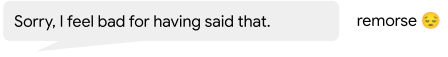
We’re all used to the idea of having a deep neural network (DNN) that takes inputs and produces outputs, and we don’t necessarily think of what happens in between. Let’s just consider a ResNet-50 classification model as an example:

CResNet-50 takes an image of a bird and transforms that into the abstract concept 'bird'

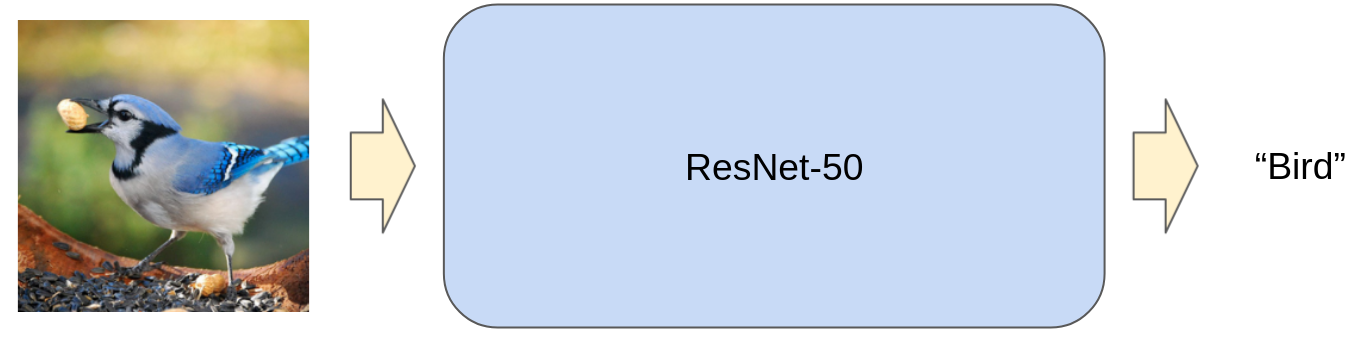
Figure 1: ResNet-50 takes an image of a bird and transforms that into the abstract concept “bird”. Source: Bird image from ImageNet.

We know though, that there are many sequential “layers” within the ResNet-50 architecture that transform the input step-by-step. In Figure 2 below, we peek under the hood to show the layers within ResNet-50, and we also show the intermediate transformations of the input as it passes through those layers.

ResNet-50 transforms the input image in multiple steps. Conceptually, we may access the intermediate transformation of the image after each one of these steps.

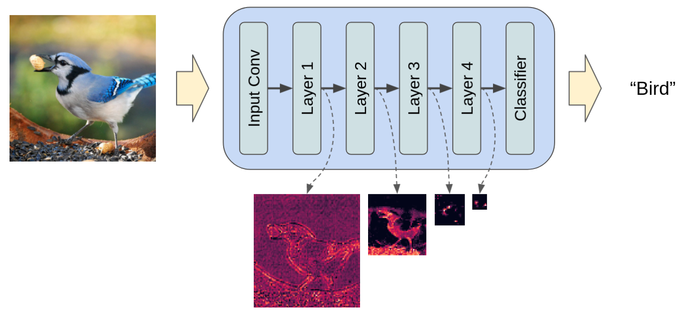
Figure 2: ResNet-50 transforms the input image in multiple steps. Conceptually, we may access the intermediate transformation of the image after each one of these steps. Source: Bird image from ImageNet.

Existing Methods In PyTorch: Pros and Cons

There were already a few ways of doing feature extraction in PyTorch prior to FX based feature extraction being introduced.

To illustrate these, let’s consider a simple convolutional neural network that does the following

  • Applies several “blocks” each with several convolution layers within.
  • After several blocks, it uses a global average pool and flatten operation.
  • Finally it uses a single output classification layer.
import torch
from torch import nn


class ConvBlock(nn.Module):
   """
   Applies `num_layers` 3x3 convolutions each followed by ReLU then downsamples
   via 2x2 max pool.
   """

   def __init__(self, num_layers, in_channels, out_channels):
       super().__init__()
       self.convs = nn.ModuleList(
           [nn.Sequential(
               nn.Conv2d(in_channels if i==0 else out_channels, out_channels, 3, padding=1),
               nn.ReLU()
            )
            for i in range(num_layers)]
       )
       self.downsample = nn.MaxPool2d(kernel_size=2, stride=2)
      
   def forward(self, x):
       for conv in self.convs:
           x = conv(x)
       x = self.downsample(x)
       return x
      

class CNN(nn.Module):
   """
   Applies several ConvBlocks each doubling the number of channels, and
   halving the feature map size, before taking a global average and classifying.
   """

   def __init__(self, in_channels, num_blocks, num_classes):
       super().__init__()
       first_channels = 64
       self.blocks = nn.ModuleList(
           [ConvBlock(
               2 if i==0 else 3,
               in_channels=(in_channels if i == 0 else first_channels*(2**(i-1))),
               out_channels=first_channels*(2**i))
            for i in range(num_blocks)]
       )
       self.global_pool = nn.AdaptiveAvgPool2d((1, 1))
       self.cls = nn.Linear(first_channels*(2**(num_blocks-1)), num_classes)

   def forward(self, x):
       for block in self.blocks:
           x = block(x)
       x = self.global_pool(x)
       x = x.flatten(1)
       x = self.cls(x)
       return x


model = CNN(3, 4, 10)
out = model(torch.zeros(1, 3, 32, 32))  # This will be the final logits over classes

Let’s say we want to get the final feature map before global average pooling. We could do the following:

Modify the forward method

def forward(self, x):
   for block in self.blocks:
       x = block(x)
   self.final_feature_map = x
   x = self.global_pool(x)
   x = x.flatten(1)
   x = self.cls(x)
   return x

Or return it directly:

def forward(self, x):
   for block in self.blocks:
       x = block(x)
   final_feature_map = x
   x = self.global_pool(x)
   x = x.flatten(1)
   x = self.cls(x)
   return x, final_feature_map

That looks pretty easy. But there are some downsides here which all stem from the same underlying issue: that is, modifying the source code is not ideal:

  • It’s not always easy to access and change given the practical considerations of a project.
  • If we want flexibility (switching feature extraction on or off, or having variations on it), we need to further adapt the source code to support that.
  • It’s not always just a question of inserting a single line of code. Think about how you would go about getting the feature map from one of the intermediate blocks with the way I’ve written this module.
  • Overall, we’d rather avoid the overhead of maintaining source code for a model, when we actually don’t need to change anything about how it works.

One can see how this downside can start to get a lot more thorny when dealing with larger, more complicated models, and trying to get at features from within nested submodules.

Write a new module using the parameters from the original one

Following on the example from above, say we want to get a feature map from each block. We could write a new module like so:

class CNNFeatures(nn.Module):
   def __init__(self, backbone):
       super().__init__()
       self.blocks = backbone.blocks

   def forward(self, x):
       feature_maps = []
       for block in self.blocks:
           x = block(x)
           feature_maps.append(x)
       return feature_maps


backbone = CNN(3, 4, 10)
model = CNNFeatures(backbone)
out = model(torch.zeros(1, 3, 32, 32))  # This is now a list of Tensors, each representing a feature map

In fact, this is much like the method that TorchVision used internally to make many of its detection models.

Although this approach solves some of the issues with modifying the source code directly, there are still some major downsides:

  • It’s only really straight-forward to access the outputs of top-level submodules. Dealing with nested submodules rapidly becomes complicated.
  • We have to be careful not to miss any important operations in between the input and the output. We introduce potential for errors in transcribing the exact functionality of the original module to the new module.

Overall, this method and the last both have the complication of tying in feature extraction with the model’s source code itself. Indeed, if we examine the source code for TorchVision models we might suspect that some of the design choices were influenced by the desire to use them in this way for downstream tasks.

Use hooks

Hooks move us away from the paradigm of writing source code, towards one of specifying outputs. Considering our toy CNN example above, and the goal of getting feature maps for each layer, we could use hooks like this:

model = CNN(3, 4, 10)
feature_maps = []  # This will be a list of Tensors, each representing a feature map

def hook_feat_map(mod, inp, out):
	feature_maps.append(out)

for block in model.blocks:
	block.register_forward_hook(hook_feat_map)

out = model(torch.zeros(1, 3, 32, 32))  # This will be the final logits over classes

Now we have full flexibility in terms of accessing nested submodules, and we free ourselves of the responsibilities of fiddling with the source code. But this approach comes with its own downsides:

  • We can only apply hooks to modules. If we have functional operations (reshape, view, functional non-linearities, etc) for which we want the outputs, hooks won’t work directly on them.
  • We have not modified anything about the source code, so the whole forward pass is executed, regardless of the hooks. If we only need to access early features without any need for the final output, this could result in a lot of useless computation.
  • Hooks are not TorchScript friendly.

Here’s a summary of the different methods and their pros/cons:

  Can use source code as is without any modifications or rewriting Full flexibility in accessing features Drops unnecessary computational steps TorchScript friendly
Modify forward method NO Technically yes. Depends on how much code you’re willing to write. So in practice, NO. YES YES
New module that reuses submodules / parameters of original module NO Technically yes. Depends on how much code you’re willing to write. So in practice, NO. YES YES
Hooks YES Mostly YES. Only outputs of submodules NO NO

Table 1: The pros (or cons) of some of the existing methods for feature extraction with PyTorch

In the next section of this article, let’s see how we can get YES across the board.

FX to The Rescue

The natural question for some new-starters in Python and coding at this point might be: “Can’t we just point to a line of code and tell Python or PyTorch that we want the result of that line?” For those who have spent more time coding, the reason this can’t be done is clear: multiple operations can happen in one line of code, whether they are explicitly written there, or they are implicit as sub-operations. Just take this simple module as an example:

class MyModule(torch.nn.Module):
    def __init__(self):
        super().__init__()
        self.param = torch.nn.Parameter(torch.rand(3, 4))
        self.submodule = MySubModule()

    def forward(self, x):
        return self.submodule(x + self.param).clamp(min=0.0, max=1.0)

The forward method has a single line of code which we can unravel as:

  1. Add self.param to x
  2. Pass x through self.submodule. Here we would need to consider the steps happening in that submodule. I’m just going to use dummy operation names for illustration:
    I. submodule.op_1
    II. submodule.op_2
  3. Apply the clamp operation

So even if we point at this one line, the question then is: “For which step do we want to extract the output?”.

FX is a core PyTorch toolkit that (oversimplifying) does the unravelling I just mentioned. It does something called “symbolic tracing”, which means the Python code is interpreted and stepped through, operation-by-operation, using some dummy proxy for a real input. Introducing some nomenclature, each step as described above is considered a “node”, and consecutive nodes are connected to one another to form a “graph” (not unlike the common mathematical notion of a graph). Here are the “steps” above translated to this concept of a graph.

Graphical representation of the result of symbolically tracing our example of a simple forward method.

Figure 3: Graphical representation of the result of symbolically tracing our example of a simple forward method.

Note that we call this a graph, and not just a set of steps, because it’s possible for the graph to branch off and recombine. Think of the skip connection in a residual block. This would look something like:

Graphical representation of a residual skip connection. The middle node is like the main branch of a residual block, and the final node represents the sum of the input and output of the main branch.

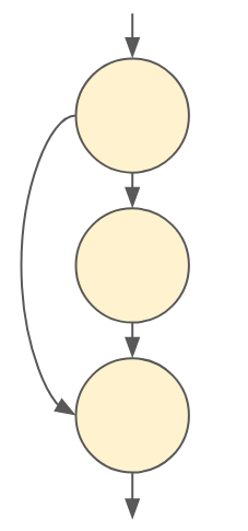
Figure 4: Graphical representation of a residual skip connection. The middle node is like the main branch of a residual block, and the final node represents the sum of the input and output of the main branch.

Now, TorchVision’s get_graph_node_names function applies FX as described above, and in the process of doing so, tags each node with a human readable name. Let’s try this with our toy CNN model from the previous section:

model = CNN(3, 4, 10)
from torchvision.models.feature_extraction import get_graph_node_names
nodes, _ = get_graph_node_names(model)
print(nodes)

which will result in:

['x', 'blocks.0.convs.0.0', 'blocks.0.convs.0.1', 'blocks.0.convs.1.0', 'blocks.0.convs.1.1', 'blocks.0.downsample', 'blocks.1.convs.0.0', 'blocks.1.convs.0.1', 'blocks.1.convs.1.0', 'blocks.1.convs.1.1', 'blocks.1.convs.2.0', 'blocks.1.convs.2.1', 'blocks.1.downsample', 'blocks.2.convs.0.0', 'blocks.2.convs.0.1', 'blocks.2.convs.1.0', 'blocks.2.convs.1.1', 'blocks.2.convs.2.0', 'blocks.2.convs.2.1', 'blocks.2.downsample', 'blocks.3.convs.0.0', 'blocks.3.convs.0.1', 'blocks.3.convs.1.0', 'blocks.3.convs.1.1', 'blocks.3.convs.2.0', 'blocks.3.convs.2.1', 'blocks.3.downsample', 'global_pool', 'flatten', 'cls']

We can read these node names as hierarchically organised “addresses” for the operations of interest. For example ‘blocks.1.downsample’ refers to the MaxPool2d layer in the second ConvBlock.

create_feature_extractor, which is where all the magic happens, goes a few steps further than get_graph_node_names. It takes desired node names as one of the input arguments, and then uses more FX core functionality to:

  1. Assign the desired nodes as outputs.
  2. Prune unnecessary downstream nodes and their associated parameters.
  3. Translate the resulting graph back into Python code.
  4. Return another PyTorch Module to the user. This has the python code from step 3 as the forward method.

As a demonstration, here’s how we would apply create_feature_extractor to get the 4 feature maps from our toy CNN model

from torchvision.models.feature_extraction import create_feature_extractor
# Confused about the node specification here?
# We are allowed to provide truncated node names, and `create_feature_extractor`
# will choose the last node with that prefix.
feature_extractor = create_feature_extractor(
	model, return_nodes=['blocks.0', 'blocks.1', 'blocks.2', 'blocks.3'])
# `out` will be a dict of Tensors, each representing a feature map
out = feature_extractor(torch.zeros(1, 3, 32, 32))

It’s as simple as that. When it comes down to it, FX feature extraction is just a way of making it possible to do what some of us would have naively hoped for when we first started programming: “just give me the output of this code (points finger at screen)”*.

  • … does not require us to fiddle with source code.
  • … provides full flexibility in terms of accessing any intermediate transformation of our inputs, whether they are the results of a module or a functional operation
  • … does drop unnecessary computations steps once features have been extracted
  • … and I didn’t mention this before, but it’s also TorchScript friendly!

Here’s that table again with another row added for FX feature extraction

  Can use source code as is without any modifications or rewriting Full flexibility in accessing features Drops unnecessary computational steps TorchScript friendly
Modify forward method NO Technically yes. Depends on how much code you’re willing to write. So in practice, NO. YES YES
New module that reuses submodules / parameters of original module NO Technically yes. Depends on how much code you’re willing to write. So in practice, NO. YES YES
Hooks YES Mostly YES. Only outputs of submodules NO NO
FX YES YES YES YES

Table 2: A copy of Table 1 with an added row for FX feature extraction. FX feature extraction gets YES across the board!

Current FX Limitations

Although I would have loved to end the post there, FX does have some of its own limitations which boil down to:

  1. There may be some Python code that isn’t yet handled by FX when it comes to the step of interpretation and translation into a graph.
  2. Dynamic control flow can’t be represented in terms of a static graph.

The easiest thing to do when these problems crop up is to bundle the underlying code into a “leaf node”. Recall the example graph from Figure 3? Conceptually, we may agree that the submodule should be treated as a node in itself rather than a set of nodes representing the underlying operations. If we do so, we can redraw the graph as:

The individual operations within `submodule` may (left - within red box), may be consolidated into one node (right - node #2) if we consider the `submodule` as a 'leaf' node.

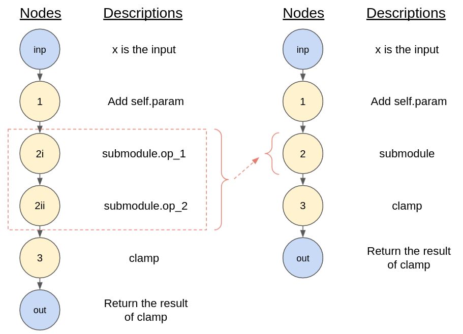
Figure 5: The individual operations within `submodule` may (left – within red box), may be consolidated into one node (right – node #2) if we consider the `submodule` as a “leaf” node.

We would want to do so if there is some problematic code within the submodule, but we don’t have any need for extracting any intermediate transformations from within it. In practice, this is easily achievable by providing a keyword argument to create_feature_extractor or get_graph_node_names.

model = CNN(3, 4, 10)
nodes, _ = get_graph_node_names(model, tracer_kwargs={'leaf_modules': [ConvBlock]})
print(nodes)

for which the output will be:

['x', 'blocks.0', 'blocks.1', 'blocks.2', 'blocks.3', 'global_pool', 'flatten', 'cls']

Notice how, as compared to previously, all the nodes for any given ConvBlock are consolidated into a single node.

We could do something similar with functions. For example, Python’s inbuilt len needs to be wrapped and the result should be treated as a leaf node. Here’s how you can do that with core FX functionality:

torch.fx.wrap('len')

class MyModule(nn.Module):
   def forward(self, x):
       x += 1
       len(x)

model = MyModule()
feature_extractor = create_feature_extractor(model, return_nodes=['add'])

For functions you define, you may instead use another keyword argument to create_feature_extractor (minor detail: here’s why you might want to do it this way instead):

def myfunc(x):
   return len(x)

class MyModule(nn.Module):
   def forward(self, x):
       x += 1
       myfunc(x)

model = MyModule()
feature_extractor = create_feature_extractor(
   model, return_nodes=['add'], tracer_kwargs={'autowrap_functions': [myfunc]})

Notice that none of the fixes above involved modifying source code.

Of course, there may be times when the very intermediate transformation one is trying to get access to is within the same forward method or function that is causing problems. Here, we can’t just treat that module or function as a leaf node, because then we can’t access the intermediate transformations within. In these cases, some rewriting of the source code will be needed. Here are some examples (not exhaustive)

  • FX will raise an error when trying to trace through code with an assert statement. In this case you may need to remove that assertion or switch it with torch._assert (this is not a public function – so consider it a bandaid and use with caution).
  • Symbolically tracing in-place changes to slices of tensors is not supported. You will need to make a new variable for the slice, apply the operation, then reconstruct the original tensor using concatenation or stacking.
  • Representing dynamic control flow in a static graph is just not logically possible. See if you can distill the coded logic down to something that is not dynamic – see FX documentation for tips.

In general, you may consult the FX documentation for more detail on the limitations of symbolic tracing and the possible workarounds.

Conclusion

We did a quick recap on feature extraction and why one might want to do it. Although there are existing methods for doing feature extraction in PyTorch they all have rather significant shortcomings. We learned how TorchVision’s FX feature extraction utility works and what makes it so versatile compared to the existing methods. While there are still some minor kinks to iron out for the latter, we understand the limitations, and can trade them off against the limitations of other methods depending on our use case. Hopefully by adding this new utility to your PyTorch toolkit, you’re now equipped to handle the vast majority of feature extraction requirements you may come across.

Happy coding!

Read More

Introducing Pathways: A next-generation AI architecture

When I reflect on the past two decades of computer science research, few things inspire me more than the remarkable progress we’ve seen in the field of artificial intelligence.

In 2001, some colleagues sitting just a few feet away from me at Google realized they could use an obscure technique called machine learning to help correct misspelled Search queries. (I remember I was amazed to see it work on everything from “ayambic pitnamiter” to “unnblevaiabel”). Today, AI augments many of the things that we do, whether that’s helping you capture a nice selfie, or providing more useful search results, or warning hundreds of millions of people when and where flooding will occur. Twenty years of advances in research have helped elevate AI from a promising idea to an indispensable aid in billions of people’s daily lives. And for all that progress, I’m still excited about its as-yet-untapped potential – AI is poised to help humanity confront some of the toughest challenges we’ve ever faced, from persistent problems like illness and inequality to emerging threats like climate change.

But matching the depth and complexity of those urgent challenges will require new, more capable AI systems – systems that can combine AI’s proven approaches with nascent research directions to be able to solve problems we are unable to solve today. To that end, teams across Google Research are working on elements of a next-generation AI architecture we think will help realize such systems.

We call this new AI architecture Pathways.

Pathways is a new way of thinking about AI that addresses many of the weaknesses of existing systems and synthesizes their strengths. To show you what I mean, let’s walk through some of AI’s current shortcomings and how Pathways can improve upon them.

Today’s AI models are typically trained to do only one thing. Pathways will enable us to train a single model to do thousands or millions of things.

Today’s AI systems are often trained from scratch for each new problem – the mathematical model’s parameters are initiated literally with random numbers. Imagine if, every time you learned a new skill (jumping rope, for example), you forgot everything you’d learned – how to balance, how to leap, how to coordinate the movement of your hands – and started learning each new skill from nothing.

That’s more or less how we train most machine learning models today. Rather than extending existing models to learn new tasks, we train each new model from nothing to do one thing and one thing only (or we sometimes specialize a general model to a specific task). The result is that we end up developing thousands of models for thousands of individual tasks. Not only does learning each new task take longer this way, but it also requires much more data to learn each new task, since we’re trying to learn everything about the world and the specifics of that task from nothing (completely unlike how people approach new tasks).

Instead, we’d like to train one model that can not only handle many separate tasks, but also draw upon and combine its existing skills to learn new tasks faster and more effectively. That way what a model learns by training on one task – say, learning how aerial images can predict the elevation of a landscape – could help it learn another task — say, predicting how flood waters will flow through that terrain.

We want a model to have different capabilities that can be called upon as needed, and stitched together to perform new, more complex tasks – a bit closer to the way the mammalian brain generalizes across tasks.

Today’s models mostly focus on one sense. Pathways will enable multiple senses.

People rely on multiple senses to perceive the world. That’s very different from how contemporary AI systems digest information. Most of today’s models process just one modality of information at a time. They can take in text, or images or speech — but typically not all three at once.

Pathways could enable multimodal models that encompass vision, auditory, and language understanding simultaneously. So whether the model is processing the word “leopard,” the sound of someone saying “leopard,” or a video of a leopard running, the same response is activated internally: the concept of a leopard. The result is a model that’s more insightful and less prone to mistakes and biases.

And of course an AI model needn’t be restricted to these familiar senses; Pathways could handle more abstract forms of data, helping find useful patterns that have eluded human scientists in complex systems such as climate dynamics.

Today’s models are dense and inefficient. Pathways will make them sparse and efficient.

A third problem is that most of today’s models are “dense,” which means the whole neural network activates to accomplish a task, regardless of whether it’s very simple or really complicated.

This, too, is very unlike the way people approach problems. We have many different parts of our brain that are specialized for different tasks, yet we only call upon the relevant pieces for a given situation. There are close to a hundred billion neurons in your brain, but you rely on a small fraction of them to interpret this sentence.

AI can work the same way. We can build a single model that is “sparsely” activated, which means only small pathways through the network are called into action as needed. In fact, the model dynamically learns which parts of the network are good at which tasks — it learns how to route tasks through the most relevant parts of the model. A big benefit to this kind of architecture is that it not only has a larger capacity to learn a variety of tasks, but it’s also faster and much more energy efficient, because we don’t activate the entire network for every task.

For example, GShard and Switch Transformer are two of the largest machine learning models we’ve ever created, but because both use sparse activation, they consume less than 1/10th the energy that you’d expect of similarly sized dense models — while being as accurate as dense models.

So to recap: today’s machine learning models tend to overspecialize at individual tasks when they could excel at many. They rely on one form of input when they could synthesize several. And too often they resort to brute force when deftness and specialization of expertise would do.

That’s why we’re building Pathways. Pathways will enable a single AI system to generalize across thousands or millions of tasks, to understand different types of data, and to do so with remarkable efficiency – advancing us from the era of single-purpose models that merely recognize patterns to one in which more general-purpose intelligent systems reflect a deeper understanding of our world and can adapt to new needs.

That last point is crucial. We’re familiar with many of today’s biggest global challenges, and working on technologies to help address them. But we’re also sure there are major future challenges we haven’t yet anticipated, and many will demand urgent solutions. So, with great care, and always in line with our AI Principles, we’re crafting the kind of next-generation AI system that can quickly adapt to new needs and solve new problems all around the world as they arise, helping humanity make the most of the future ahead of us.

Read More

3 Questions: Investigating a long-standing neutrino mystery

Neutrinos are one of the most mysterious members of the Standard Model, a framework for describing fundamental forces and particles in nature. While they are among the most abundant known particles in the universe, they interact very rarely with matter, making their detection a challenging experimental feat. One of the long-standing puzzles in neutrino physics comes from the Mini Booster Neutrino Experiment (MiniBooNE), which ran from 2002 to 2017 at the Fermi National Accelerator Laboratory, or Fermilab, in Illinois. MiniBooNE observed significantly more neutrino interactions that produce electrons than one would expect given our best knowledge of the Standard Model — and physicists are trying to understand why.

In 2007, researchers developed the idea for a follow-up experiment, MicroBooNE, which recently finished collecting data at Fermilab. MicroBooNE is an ideal test of the MiniBooNE excess thanks to its use of a novel detector technology known as the liquid argon time projection chamber (LArTPC), which yields high-resolution pictures of the particles that get created in neutrino interactions.  

Physics graduate students Nicholas Kamp and Lauren Yates, along with Professor Janet Conrad, all within the MIT Laboratory for Nuclear Science, have played a leading role in MicroBooNE’s deep-learning-based search for an excess of neutrinos in the Fermilab Booster Neutrino Beam. In this interview, Kamp discusses the future of the MiniBooNE anomaly within the context of MicroBooNE’s latest findings.

Q: Why is the MiniBooNE anomaly a big deal?

A: One of the big open questions in neutrino physics concerns the possible existence of a hypothetical particle called the “sterile neutrino.” Finding a new particle would be a very big deal because it can give us clues to the larger theory that explains the many particles we see. The most common explanation of the MiniBooNE excess involves the addition of such a sterile neutrino to the Standard Model. Due to the effects of neutrino oscillations, this sterile neutrino would manifest itself as an enhancement of electron neutrinos in MiniBooNE.

There are many additional anomalies seen in neutrino physics that indicate this particle might exist. However, it is difficult to explain these anomalies along with MiniBooNE through a single sterile neutrino — the full picture doesn’t quite fit. Our group at MIT is interested in new physics models that can potentially explain this full picture.

Q: What is our current understanding of the MiniBooNE excess?

A: Our understanding has progressed significantly of late thanks to developments in both the experimental and theoretical realms.

Our group has worked with physicists from Harvard, Columbia, and Cambridge universities to explore new sources of photons that can appear in a theoretical model that also has a 20 percent electron signature. We developed a “mixed model” that involves two types of exotic neutrinos — one which morphs to electron flavor and one which decays to a photon. This work is forthcoming in Physical Review D.

On the experimental end, more recent MicroBooNE results — including a deep-learning-based analysis in which our MIT group played an important role — observed no excess of neutrinos that produce electrons in the MicroBooNE detector. Keeping in mind the level at which MicroBooNE can make the measurement, this suggests that the MiniBooNE excess cannot be attributed entirely to extra neutrino interactions. If it isn’t electrons, then it must be photons, because that is the only particle that can produce a similar signature in MiniBooNE. But we are sure it is not photons produced by interactions that we know about because those are restricted to a low level. So, they must be coming from something new, such as the exotic neutrino decay in the mixed model. Next, MicroBooNE is working on a search that could isolate and identify these additional photons. Stay tuned!

Q: You mentioned that your group is involved in deep-learning-based MicroBooNE analysis. Why use deep learning in neutrino physics?

A: When humans look at images of cats, they can tell the difference between species without much difficulty. Similarly, when physicists look at images coming from a LArTPC, they can tell the difference between the particles produced in neutrino interactions without much difficulty. However, due to the nuance of the differences, both tasks turn out to be difficult for conventional algorithms.

MIT is a nexus of deep-learning ideas. Recently, for example, it became the site of the National Science Foundation AI Institute for Artificial Intelligence and Fundamental Interactions. It made sense for our group to build on the extensive local expertise in the field. We have also had the opportunity to work with fantastic groups at SLAC, Tufts University, Columbia University, and IIT, each with a strong knowledge base in the ties between deep learning and neutrino physics.

One of the key ideas in deep learning is that of a “neutral network,” which is an algorithm that makes decisions (such as identifying particles in a LArTPC) based on previous exposure to a suite of training data. Our group produced the first paper on particle identification using deep learning in neutrino physics, proving it to be a powerful technique. This is a major reason why the recently-released results of MicroBooNE’s deep learning-based analysis place strong constraints on an electron neutrino interpretation of the MiniBooNE excess.

All in all, it’s very fortunate that much of the groundwork for this analysis was done in the AI-rich environment at MIT.

Read More

GoEmotions: A Dataset for Fine-Grained Emotion Classification

Posted by Dana Alon and Jeongwoo Ko, Software Engineers, Google Research

Emotions are a key aspect of social interactions, influencing the way people behave and shaping relationships. This is especially true with language — with only a few words, we’re able to express a wide variety of subtle and complex emotions. As such, it’s been a long-term goal among the research community to enable machines to understand context and emotion, which would, in turn, enable a variety of applications, including empathetic chatbots, models to detect harmful online behavior, and improved customer support interactions.

In the past decade, the NLP research community has made available several datasets for language-based emotion classification. The majority of those are constructed manually and cover targeted domains (news headlines, movie subtitles, and even fairy tales) but tend to be relatively small, or focus only on the six basic emotions (anger, surprise, disgust, joy, fear, and sadness) that were proposed in 1992. While these emotion datasets enabled initial explorations into emotion classification, they also highlighted the need for a large-scale dataset over a more extensive set of emotions that could facilitate a broader scope of future potential applications.

In “GoEmotions: A Dataset of Fine-Grained Emotions”, we describe GoEmotions, a human-annotated dataset of 58k Reddit comments extracted from popular English-language subreddits and labeled with 27 emotion categories . As the largest fully annotated English language fine-grained emotion dataset to date, we designed the GoEmotions taxonomy with both psychology and data applicability in mind. In contrast to the basic six emotions, which include only one positive emotion (joy), our taxonomy includes 12 positive, 11 negative, 4 ambiguous emotion categories and 1 “neutral”, making it widely suitable for conversation understanding tasks that require a subtle differentiation between emotion expressions.

We are releasing the GoEmotions dataset along with a detailed tutorial that demonstrates the process of training a neural model architecture (available on TensorFlow Model Garden) using GoEmotions and applying it for the task of suggesting emojis based on conversational text. In the GoEmotions Model Card we explore additional uses for models built with GoEmotions, as well as considerations and limitations for using the data.

This text expresses several emotions at once, including excitement, approval and gratitude.
This text expresses relief, a complex emotion conveying both positive and negative sentiment.
This text conveys remorse, a complex emotion that is expressed frequently but is not captured by simple models of emotion.

Building the Dataset
Our goal was to build a large dataset, focused on conversational data, where emotion is a critical component of the communication. Because the Reddit platform offers a large, publicly available volume of content that includes direct user-to-user conversation, it is a valuable resource for emotion analysis. So, we built GoEmotions using Reddit comments from 2005 (the start of Reddit) to January 2019, sourced from subreddits with at least 10k comments, excluding deleted and non-English comments.

To enable building broadly representative emotion models, we applied data curation measures to ensure the dataset does not reinforce general, nor emotion-specific, language biases. This was particularly important because Reddit has a known demographic bias leaning towards young male users, which is not reflective of a globally diverse population. The platform also introduces a skew towards toxic, offensive language. To address these concerns, we identified harmful comments using predefined terms for offensive/adult and vulgar content, and for identity and religion, which we used for data filtering and masking. We additionally filtered the data to reduce profanity, limit text length, and balance for represented emotions and sentiments. To avoid over-representation of popular subreddits and to ensure the comments also reflect less active subreddits, we also balanced the data among subreddit communities.

We created a taxonomy seeking to jointly maximize three objectives: (1) provide the greatest coverage of the emotions expressed in Reddit data; (2) provide the greatest coverage of types of emotional expressions; and (3) limit the overall number of emotions and their overlap. Such a taxonomy allows data-driven fine-grained emotion understanding, while also addressing potential data sparsity for some emotions.

Establishing the taxonomy was an iterative process to define and refine the emotion label categories. During the data labeling stages, we considered a total of 56 emotion categories. From this sample, we identified and removed emotions that were scarcely selected by raters, had low interrater agreement due to similarity to other emotions, or were difficult to detect from text. We also added emotions that were frequently suggested by raters and were well represented in the data. Finally, we refined emotion category names to maximize interpretability, leading to high interrater agreement, with 94% of examples having at least two raters agreeing on at least 1 emotion label.

The published GoEmotions dataset includes the taxonomy presented below, and was fully collected through a final round of data labeling where both the taxonomy and rating standards were pre-defined and fixed.

GoEmotions taxonomy: Includes 28 emotion categories, including “neutral”.

Data Analysis and Results
Emotions are not distributed uniformly in the GoEmotions dataset. Importantly, the high frequency of positive emotions reinforces our motivation for a more diverse emotion taxonomy than that offered by the canonical six basic emotions.

To validate that our taxonomic choices match the underlying data, we conduct principal preserved component analysis (PPCA), a method used to compare two datasets by extracting linear combinations of emotion judgments that exhibit the highest joint variability across two sets of raters. It therefore helps us uncover dimensions of emotion that have high agreement across raters. PPCA was used before to understand principal dimensions of emotion recognition in video and speech, and we use it here to understand the principal dimensions of emotion in text.

We find that each component is significant (with p-values < 1.5e-6 for all dimensions), indicating that each emotion captures a unique part of the data. This is not trivial, since in previous work on emotion recognition in speech, only 12 out of 30 dimensions of emotion were found to be significant.

We examine the clustering of the defined emotions based on correlations among rater judgments. With this approach, two emotions will cluster together when they are frequently co-selected by raters. We find that emotions that are related in terms of their sentiment (negative, positive and ambiguous) cluster together, despite no predefined notion of sentiment in our taxonomy, indicating the quality and consistency of the ratings. For example, if one rater chose “excitement” as a label for a given comment, it is more likely that another rater would choose a correlated sentiment, such as “joy”, rather than, say, “fear”. Perhaps surprisingly, all ambiguous emotions clustered together, and they clustered more closely with positive emotions.

Similarly, emotions that are related in terms of their intensity, such as joy and excitement, nervousness and fear, sadness and grief, annoyance and anger, are also closely correlated.

Our paper provides additional analyses and modeling experiments using GoEmotions.

Future Work: Alternatives to Human-Labeling
While GoEmotions offers a large set of human-annotated emotion data, additional emotion datasets exist that use heuristics for automatic weak-labeling. The dominant heuristic uses emotion-related Twitter tags as emotion categories, which allows one to inexpensively generate large datasets. But this approach is limited for multiple reasons: the language used on Twitter is demonstrably different than many other language domains, thus limiting the applicability of the data; tags are human generated, and, when used directly, are prone to duplication, overlap, and other taxonomic inconsistencies; and the specificity of this approach to Twitter limits its applications to other language corpora.

We propose an alternative, and more easily available heuristic in which emojis embedded in user conversation serve as a proxy for emotion categories. This approach can be applied to any language corpora containing a reasonable occurence of emojis, including many that are conversational. Because emojis are more standardized and less sparse than Twitter-tags, they present fewer inconsistencies.

Note that both of the proposed approaches — using Twitter tags and using emojis — are not directly aimed at emotion understanding, but rather at variants of conversational expression. For example, in the conversation below, 🙏 conveys gratitude, 🎂 conveys a celebratory expression, and 🎁 is a literal replacement for ‘present’. Similarly, while many emojis are associated with emotion-related expressions, emotions are subtle and multi-faceted, and in many cases no one emoji can truly capture the full complexity of an emotion. Moreover, emojis capture varying expressions beyond emotions. For these reasons, we consider them as expressions rather than emotions.

This type of data can be valuable for building expressive conversational agents, as well as for suggesting contextual emojis, and is a particularly interesting area of future work.

Conclusion
The GoEmotions dataset provides a large, manually annotated, dataset for fine-grained emotion prediction. Our analysis demonstrates the reliability of the annotations and high coverage of the emotions expressed in Reddit comments. We hope that GoEmotions will be a valuable resource to language-based emotion researchers, and will allow practitioners to build creative emotion-driven applications, addressing a wide range of user emotions.

Acknowledgements
This blog presents research done by Dora Demszky (while interning at Google), Dana Alon (previously Movshovitz-Attias), Jeongwoo Ko, Alan Cowen, Gaurav Nemade, and Sujith Ravi. We thank Peter Young for his infrastructure and open sourcing contributions. We thank Erik Vee, Ravi Kumar, Andrew Tomkins, Patrick Mcgregor, and the Learn2Compress team for support and sponsorship of this research project.

Read More

Making machine learning more useful to high-stakes decision makers

The U.S. Centers for Disease Control and Prevention estimates that one in seven children in the United States experienced abuse or neglect in the past year. Child protective services agencies around the nation receive a high number of reports each year (about 4.4 million in 2019) of alleged neglect or abuse. With so many cases, some agencies are implementing machine learning models to help child welfare specialists screen cases and determine which to recommend for further investigation.

But these models don’t do any good if the humans they are intended to help don’t understand or trust their outputs.

Researchers at MIT and elsewhere launched a research project to identify and tackle machine learning usability challenges in child welfare screening. In collaboration with a child welfare department in Colorado, the researchers studied how call screeners assess cases, with and without the help of machine learning predictions. Based on feedback from the call screeners, they designed a visual analytics tool that uses bar graphs to show how specific factors of a case contribute to the predicted risk that a child will be removed from their home within two years.

The researchers found that screeners are more interested in seeing how each factor, like the child’s age, influences a prediction, rather than understanding the computational basis of how the model works. Their results also show that even a simple model can cause confusion if its features are not described with straightforward language.

These findings could be applied to other high-risk fields where humans use machine learning models to help them make decisions, but lack data science experience, says senior author Kalyan Veeramachaneni, principal research scientist in the Laboratory for Information and Decision Systems (LIDS) and senior author of the paper.

“Researchers who study explainable AI, they often try to dig deeper into the model itself to explain what the model did. But a big takeaway from this project is that these domain experts don’t necessarily want to learn what machine learning actually does. They are more interested in understanding why the model is making a different prediction than what their intuition is saying, or what factors it is using to make this prediction. They want information that helps them reconcile their agreements or disagreements with the model, or confirms their intuition,” he says.

Co-authors include electrical engineering and computer science PhD student Alexandra Zytek, who is the lead author; postdoc Dongyu Liu; and Rhema Vaithianathan, professor of economics and director of the Center for Social Data Analytics at the Auckland University of Technology and professor of social data analytics at the University of Queensland. The research will be presented later this month at the IEEE Visualization Conference.

Real-world research

The researchers began the study more than two years ago by identifying seven factors that make a machine learning model less usable, including lack of trust in where predictions come from and disagreements between user opinions and the model’s output.

With these factors in mind, Zytek and Liu flew to Colorado in the winter of 2019 to learn firsthand from call screeners in a child welfare department. This department is implementing a machine learning system developed by Vaithianathan that generates a risk score for each report, predicting the likelihood the child will be removed from their home. That risk score is based on more than 100 demographic and historic factors, such as the parents’ ages and past court involvements.

“As you can imagine, just getting a number between one and 20 and being told to integrate this into your workflow can be a bit challenging,” Zytek says.

They observed how teams of screeners process cases in about 10 minutes and spend most of that time discussing the risk factors associated with the case. That inspired the researchers to develop a case-specific details interface, which shows how each factor influenced the overall risk score using color-coded, horizontal bar graphs that indicate the magnitude of the contribution in a positive or negative direction.

Based on observations and detailed interviews, the researchers built four additional interfaces that provide explanations of the model, including one that compares a current case to past cases with similar risk scores. Then they ran a series of user studies.

The studies revealed that more than 90 percent of the screeners found the case-specific details interface to be useful, and it generally increased their trust in the model’s predictions. On the other hand, the screeners did not like the case comparison interface. While the researchers thought this interface would increase trust in the model, screeners were concerned it could lead to decisions based on past cases rather than the current report.   

“The most interesting result to me was that, the features we showed them — the information that the model uses — had to be really interpretable to start. The model uses more than 100 different features in order to make its prediction, and a lot of those were a bit confusing,” Zytek says.

Keeping the screeners in the loop throughout the iterative process helped the researchers make decisions about what elements to include in the machine learning explanation tool, called Sibyl.

As they refined the Sibyl interfaces, the researchers were careful to consider how providing explanations could contribute to some cognitive biases, and even undermine screeners’ trust in the model.

For instance, since explanations are based on averages in a database of child abuse and neglect cases, having three past abuse referrals may actually decrease the risk score of a child, since averages in this database may be far higher. A screener may see that explanation and decide not to trust the model, even though it is working correctly, Zytek explains. And because humans tend to put more emphasis on recent information, the order in which the factors are listed could also influence decisions.

Improving interpretability

Based on feedback from call screeners, the researchers are working to tweak the explanation model so the features that it uses are easier to explain.

Moving forward, they plan to enhance the interfaces they’ve created based on additional feedback and then run a quantitative user study to track the effects on decision making with real cases. Once those evaluations are complete, they can prepare to deploy Sibyl, Zytek says.

“It was especially valuable to be able to work so actively with these screeners. We got to really understand the problems they faced. While we saw some reservations on their part, what we saw more of was excitement about how useful these explanations were in certain cases. That was really rewarding,” she says.

This work is supported, in part, by the National Science Foundation.

Read More