Monthly Archives: September 2023

This guest post is co-written by Lydia Lihui Zhang, Business Development Specialist, and Mansi Shah, Software Engineer/Data Scientist, at Planet Labs. The analysis that inspired this post was originally written by Jennifer Reiber Kyle.

Amazon SageMaker geospatial capabilities combined with Planet’s satellite data can be used for crop segmentation, and there are numerous applications and potential benefits of this analysis to the fields of agriculture and sustainability. In late 2023, Planet announced a partnership with AWS to make its geospatial data available through Amazon SageMaker.

Crop segmentation is the process of splitting up a satellite image into regions of pixels, or segments, that have similar crop characteristics. In this post, we illustrate how to use a segmentation machine learning (ML) model to identify crop and non-crop regions in an image.

Identifying crop regions is a core step towards gaining agricultural insights, and the combination of rich geospatial data and ML can lead to insights that drive decisions and actions. For example:

• Making data-driven farming decisions – By gaining better spatial understanding of the crops, farmers and other agricultural stakeholders can optimize the use of resources, from water to fertilizer to other chemicals across the season. This sets the foundation for reducing waste, improving sustainable farming practices wherever possible, and increasing productivity while minimizing environmental impact.
• Identifying climate-related stresses and trends – As climate change continues to affect global temperature and rainfall patterns, crop segmentation can be used to identify areas that are vulnerable to climate-related stress for climate adaptation strategies. For example, satellite imagery archives can be used to track changes in a crop growing region over time. These could be the physical changes in size and distribution of croplands. They could also be the changes in soil moisture, soil temperature, and biomass, derived from the different spectral index of satellite data, for deeper crop health analysis.
• Assessing and mitigating damage – Finally, crop segmentation can be used to quickly and accurately identify areas of crop damage in the event of a natural disaster, which can help prioritize relief efforts. For example, after a flood, high-cadence satellite images can be used to identify areas where crops have been submerged or destroyed, allowing relief organizations to assist affected farmers more quickly.

In this analysis, we use a K-nearest neighbors (KNN) model to conduct crop segmentation, and we compare these results with ground truth imagery on an agricultural region. Our results reveal that the classification from the KNN model is more accurately representative of the state of the current crop field in 2017 than the ground truth classification data from 2015. These results are a testament to the power of Planet’s high-cadence geospatial imagery. Agricultural fields change often, sometimes multiple times a season, and having high-frequency satellite imagery available to observe and analyze this land can provide immense value to our understanding of agricultural land and quickly-changing environments.

Planet and AWS’s partnership on geospatial ML

SageMaker geospatial capabilities empower data scientists and ML engineers to build, train, and deploy models using geospatial data. SageMaker geospatial capabilities allow you to efficiently transform or enrich large-scale geospatial datasets, accelerate model building with pre-trained ML models, and explore model predictions and geospatial data on an interactive map using 3D-accelerated graphics and built-in visualization tools. With SageMaker geospatial capabilities, you can process large datasets of satellite imagery and other geospatial data to create accurate ML models for various applications, including crop segmentation, which we discuss in this post.

Planet Labs PBC is a leading Earth-imaging company that uses its large fleet of satellites to capture imagery of the Earth’s surface on a daily basis. Planet’s data is therefore a valuable resource for geospatial ML. Its high-resolution satellite imagery can be used to identify various crop characteristics and their health over time, anywhere on Earth.

The partnership between Planet and SageMaker enables customers to easily access and analyze Planet’s high-frequency satellite data using AWS’s powerful ML tools. Data scientists can bring their own data or conveniently find and subscribe to Planet’s data without switching environments.

Crop segmentation in an Amazon SageMaker Studio notebook with a geospatial image

In this example geospatial ML workflow, we look at how to bring Planet’s data along with the ground truth data source into SageMaker, and how to train, infer, and deploy a crop segmentation model with a KNN classifier. Finally, we assess the accuracy of our results and compare this to our ground truth classification.

The KNN classifier used was trained in an Amazon SageMaker Studio notebook with a geospatial image, and provides a flexible and extensible notebook kernel for working with geospatial data.

The Amazon SageMaker Studio notebook with geospatial image comes pre-installed with commonly used geospatial libraries such as GDAL, Fiona, GeoPandas, Shapely, and Rasterio, which allow the visualization and processing of geospatial data directly within a Python notebook environment. Common ML libraries such as OpenCV or scikit-learn are also used to perform crop segmentation using KNN classification, and these are also installed in the geospatial kernel.

Data selection

The agricultural field we zoom into is located at the usually sunny Sacramento County in California.

Why Sacramento? The area and time selection for this type of problem is primarily defined by the availability of ground truth data, and such data in crop type and boundary data, is not easy to come by. The 2015 Sacramento County Land Use DWR Survey dataset is a publicly available dataset covering Sacramento County in that year and provides hand-adjusted boundaries.

The primary satellite imagery we use is the Planet’s 4-band PSScene Product, which contains the Blue, Green, Red, and Near-IR bands and is radiometrically corrected to at-sensor radiance. The coefficients for correcting to at-sensor reflectance are provided in the scene metadata, which further improves the consistency between images taken at different times.

Planet’s Dove satellites that produced this imagery were launched February 14, 2017 (news release), therefore they didn’t image Sacramento County back in 2015. However, they have been taking daily imagery of the area since the launch. In this example, we settle for the imperfect 2-year gap between the ground truth data and satellite imagery. However, Landsat 8 lower-resolution imagery could have been used as a bridge between 2015 and 2017.

Access Planet data

To help users get accurate and actionable data faster, Planet has also developed the Planet Software Development Kit (SDK) for Python. This is a powerful tool for data scientists and developers who want to work with satellite imagery and other geospatial data. With this SDK, you can search and access Planet’s vast collection of high-resolution satellite imagery, as well as data from other sources like OpenStreetMap. The SDK provides a Python client to Planet’s APIs, as well as a no-code command line interface (CLI) solution, making it easy to incorporate satellite imagery and geospatial data into Python workflows. This example uses the Python client to identify and download imagery needed for the analysis.

You can install the Planet Python client in the SageMaker Studio notebook with geospatial image using a simple command:

%pip install planet

You can use the client to query relevant satellite imagery and retrieve a list of available results based on the area of interest, time range, and other search criteria. In the following example, we start by asking how many PlanetScope scenes (Planet’s daily imagery) cover the same area of interest (AOI) that we define earlier through the ground data in Sacramento, given a certain time range between June 1 and October 1, 2017; as well as a certain desired maximum cloud coverage range of 10%:

# create a request using the SDK from the search specifications of the data

item_type = ['PSScene']

geom_filter_train = data_filter.geometry_filter(aoi_train)
date_range_filter = data_filter.date_range_filter("acquired", gt=datetime(month=6, day=1, year=2017), lt=datetime(month=10, day=1, year=2017))
cloud_cover_filter = data_filter.range_filter('cloud_cover', lt=0.10)

combined_filter_test = data_filter.and_filter([geom_filter_test, date_range_filter, cloud_cover_filter])
    
# Run a quick search for our TRAIN data
async with Session() as sess:
    cl = sess.client('data')
    results = cl.search(name='temp_search_train',search_filter=combined_filter_train, item_types=item_type)
    train_result_list = [i async for i in results]

print("Number of train scene results: ", len(train_result_list))

The returned results show the number of matching scenes overlapping with our area of interest. It also contains each scene’s metadata, its image ID, and a preview image reference.

After a particular scene has been selected, with specification on the scene ID, item type, and product bundles (reference documentation), you can use the following code to download the image and its metadata:

train_scene_id = '20170601_180425_0f35'
item_type = 'PSScene'
bundle_type = 'analytic_sr_udm2'

# define the order request
products = [order_request.product([train_scene_id], bundle_type, item_type)]
request = order_request.build_request('train_dataset', products=products)

# download the training data
async with Session() as sess:
    cl = sess.client('orders')
    # use "reporting" to manage polling for order status
    with reporting.StateBar(state='creating') as bar:
        # perform the order with the prior created order request
        order = await cl.create_order(request)
        bar.update(state='created', order_id=train_order['id'])

        # wait via polling until the order is processed
        await cl.wait(train_order['id'], callback=bar.update_state)

    #  download the actual asset
    await cl.download_order(order_id=order['id'], directory=download_directory, progress_bar=True, overwrite=True)

This code downloads the corresponding satellite image to the Amazon Elastic File System (Amazon EFS) volume for SageMaker Studio.

Model training

After the data has been downloaded with the Planet Python client, the segmentation model can be trained. In this example, a combination of KNN classification and image segmentation techniques is used to identify crop area and create georeferenced geojson features.

The Planet data is loaded and preprocessed using the built-in geospatial libraries and tools in SageMaker to prepare it for training the KNN classifier. The ground truth data for training is the Sacramento County Land Use DWR Survey dataset from 2015, and the Planet data from 2017 is used for testing the model.

Convert ground truth features to contours

To train the KNN classifier, the class of each pixel as either crop or non-crop needs to be identified. The class is determined by whether the pixel is associated with a crop feature in the ground truth data or not. To make this determination, the ground truth data is first converted into OpenCV contours, which are then used to separate crop from non-crop pixels. The pixel values and their classification are then used to train the KNN classifier.

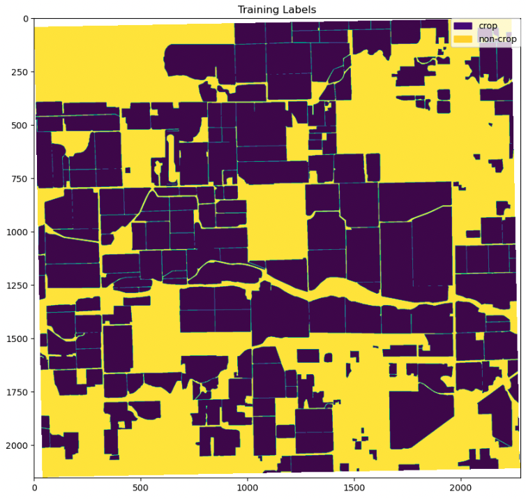
To convert the ground truth features to contours, the features must first be projected to the coordinate reference system of the image. Then, the features are transformed into image space, and finally converted into contours. To ensure the accuracy of the contours, they are visualized overlaid on the input image, as shown in the following example.

To train the KNN classifier, crop and non-crop pixels are separated using the crop feature contours as a mask.

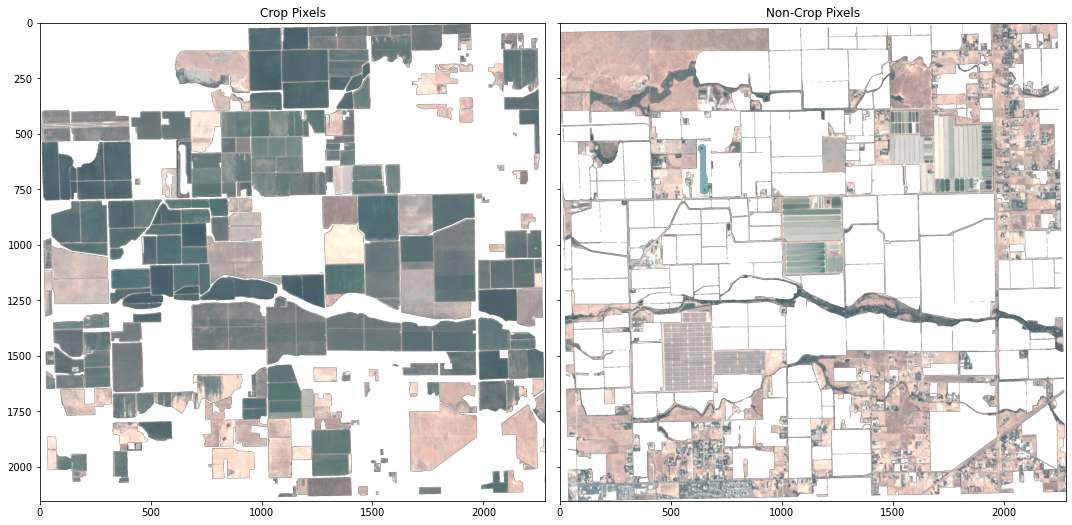
The input of KNN classifier consists of two datasets: X, a 2d array that provides the features to be classified on; and y, a 1d array that provides the classes (example). Here, a single classified band is created from the non-crop and crop datasets, where the band’s values indicate the pixel class. The band and the underlying image pixel band values are then converted to the X and y inputs for the classifier fit function.

Train the classifier on crop and non-crop pixels

The KNN classification is performed with the scikit-learn KNeighborsClassifier. The number of neighbors, a parameter greatly affecting the estimator’s performance, is tuned using cross-validation in KNN cross-validation. The classifier is then trained using the prepared datasets and the tuned number of neighbor parameters. See the following code:

def fit_classifier(pl_filename, ground_truth_filename, metadata_filename, n_neighbors):
    weights = 'uniform'
    clf = neighbors.KNeighborsClassifier(n_neighbors, weights=weights)
    train_class_band = create_contour_classified_band(pl_filename, ground_truth_filename)
    X = to_X(load_refl_bands(pl_filename, metadata_filename))
    y = to_y(train_class_band)
    clf.fit(X, y)
    return clf

clf = fit_classifier(train_scene_filename,
                     train_ground_truth_filename,
                     train_metadata_filename,
                     n_neighbors)

To assess the classifier’s performance on its input data, the pixel class is predicted using the pixel band values. The classifier’s performance is mainly based on the accuracy of the training data and the clear separation of the pixel classes based on the input data (pixel band values). The classifier’s parameters, such as the number of neighbors and the distance weighting function, can be adjusted to compensate for any inaccuracies in the latter. See the following code:

def predict(pl_filename, metadata_filename, clf):
    bands = load_refl_bands(pl_filename, metadata_filename)
    X = to_X(bands)
    y = clf.predict(X)
    return classified_band_from_y(bands[0].mask, y)

train_predicted_class_band = predict(train_scene_filename, train_metadata_filename, clf)

Evaluate model predictions

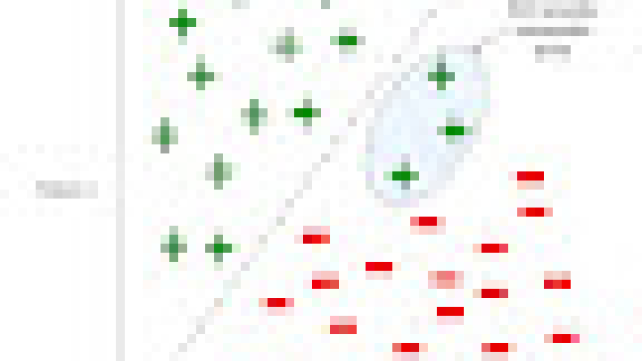
The trained KNN classifier is utilized to predict crop regions in the test data. This test data consists of regions that were not exposed to the model during training. In other words, the model has no knowledge of the area prior to its analysis and therefore this data can be used to objectively evaluate the model’s performance. We start by visually inspecting several regions, beginning with a region that is comparatively noisier.

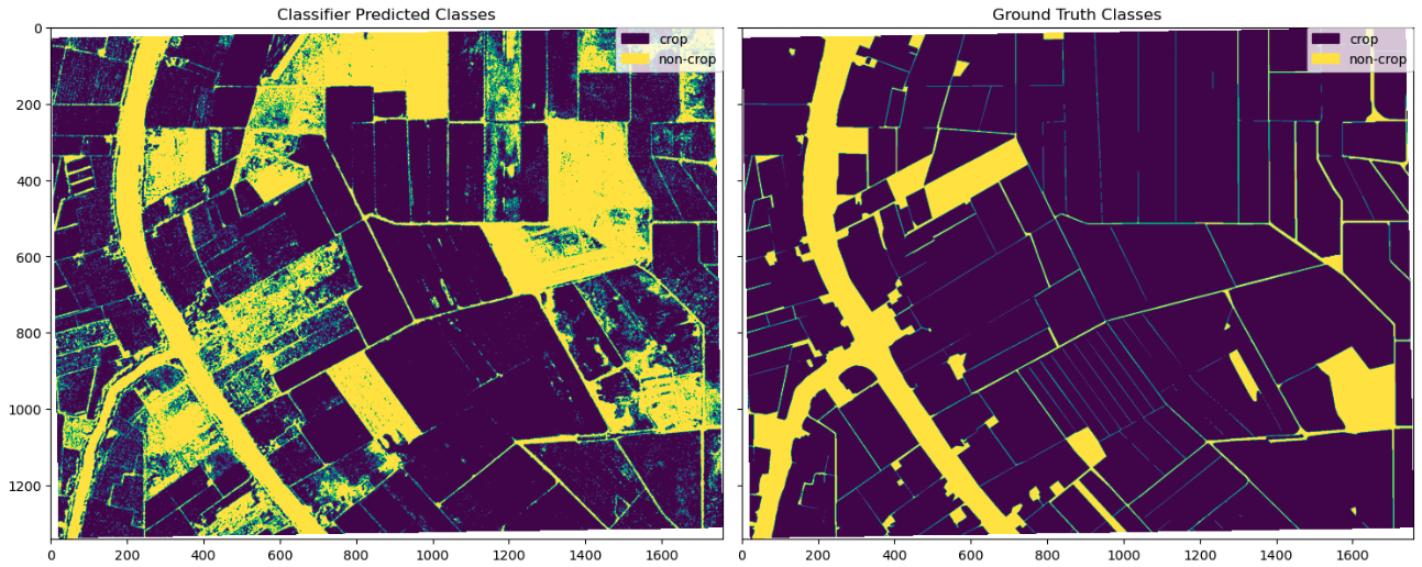
The visual inspection reveals that the predicted classes are mostly consistent with the ground truth classes. There are a few regions of deviation, which we inspect further.

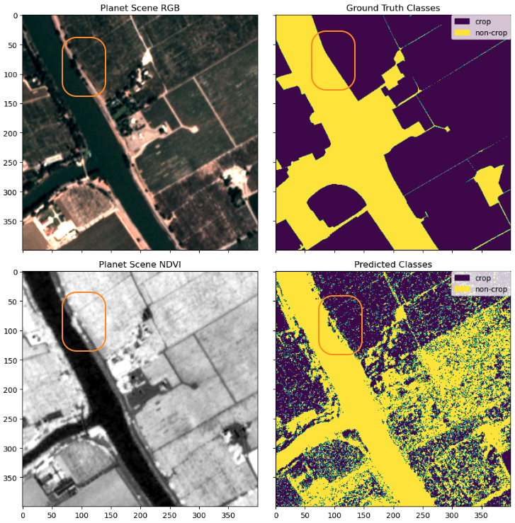
Upon further investigation, we discovered that some of the noise in this region was due to the ground truth data lacking the detail that is present in the classified image (top right compared to top left and bottom left). A particularly interesting finding is that the classifier identifies trees along the river as non-crop, whereas the ground truth data mistakenly identifies them as crop. This difference between these two segmentations may be due to the trees shading the region over the crops.

Following this, we inspect another region that was classified differently between the two methods. These highlighted regions were previously marked as non-crop regions in the ground truth data in 2015 (top right) but changed and shown clearly as cropland in 2017 through the Planetscope Scenes (top left and bottom left). They were also classified largely as cropland through the classifier (bottom right).

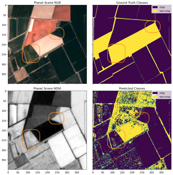
Again, we see the KNN classifier presents a more granular result than the ground truth class, and it also successfully captures the change happening in the cropland. This example also speaks to the value of daily refreshed satellite data because the world often changes much faster than annual reports, and a combined method with ML like this can help us pick up the changes as they happen. Being able to monitor and discover such changes via satellite data, especially in the evolving agricultural fields, provides helpful insights for farmers to optimize their work and any agricultural stakeholder in the value chain to get a better pulse of the season.

Model evaluation

The visual comparison of the images of the predicted classes to the ground truth classes can be subjective and can’t be generalized for assessing the accuracy of the classification results. To obtain a quantitative assessment, we obtain classification metrics by using scikit-learn’s classification_report function:

# train dataset
print(classification_report(to_y(create_contour_classified_band(train_scene_filename,
                                          train_ground_truth_filename)),
                            to_y(train_predicted_class_band),
                            target_names=['crop', 'non-crop']))

              precision    recall  f1-score   support

        crop       0.89      0.86      0.87   2641818
    non-crop       0.83      0.86      0.84   2093907

    accuracy                           0.86   4735725
   macro avg       0.86      0.86      0.86   4735725
weighted avg       0.86      0.86      0.86   4735725



# test dataset
print(classification_report(to_y(create_contour_classified_band(test_scene_filename,
                                       test_ground_truth_filename)),
                            to_y(test_predicted_class_band),
                            target_names=['crop', 'non-crop']))

              precision    recall  f1-score   support

        crop       0.94      0.73      0.82   1959630
    non-crop       0.32      0.74      0.44    330938

    accuracy                           0.73   2290568
   macro avg       0.63      0.74      0.63   2290568
weighted avg       0.85      0.73      0.77   2290568

The pixel classification is used to create a segmentation mask of crop regions, making both precision and recall important metrics, and the F1 score a good overall measure for predicting accuracy. Our results give us metrics for both crop and non-crop regions in the train and test dataset. However, to keep things simple, let’s take a closer look at these metrics in the context of the crop regions in the test dataset.

Precision is a measure of how accurate our model’s positive predictions are. In this case, a precision of 0.94 for crop regions indicates that our model is very successful at correctly identifying areas that are indeed crop regions, where false positives (actual non-crop regions incorrectly identified as crop regions) are minimized. Recall, on the other hand, measures the completeness of positive predictions. In other words, recall measures the proportion of actual positives that were identified correctly. In our case, a recall value of 0.73 for crop regions means that 73% of all true crop region pixels are correctly identified, minimizing the number of false negatives.

Ideally, high values of both precision and recall are preferred, although this can be largely dependent on the application of the case study. For example, if we were examining these results for farmers looking to identify crop regions for agriculture, we would want to give preference to a higher recall than precision, in order to minimize the number of false negatives (areas identified as non-crop regions that are actually crop regions) in order to make the most use of the land. The F1-score serves as an overall accuracy metric combining both precision and recall, and measuring the balance between the two metrics. A high F1-score, such as ours for crop regions (0.82), indicates a good balance between both precision and recall and a high overall classification accuracy. Although the F1-score drops between the train and test datasets, this is expected because the classifier was trained on the train dataset. An overall weighted average F1 score of 0.77 is promising and adequate enough to try segmentation schemes on the classified data.

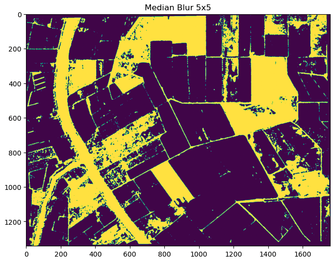
Create a segmentation mask from the classifier

The creation of a segmentation mask using the predictions from the KNN classifier on the test dataset involves cleaning up the predicted output to avoid small segments caused by image noise. To remove speckle noise, we use the OpenCV median blur filter. This filter preserves road delineations between crops better than the morphological open operation.

To apply binary segmentation to the denoised output, we first need to convert the classified raster data to vector features using the OpenCV findContours function.

Finally, the actual segmented crop regions can be computed using the segmented crop outlines.

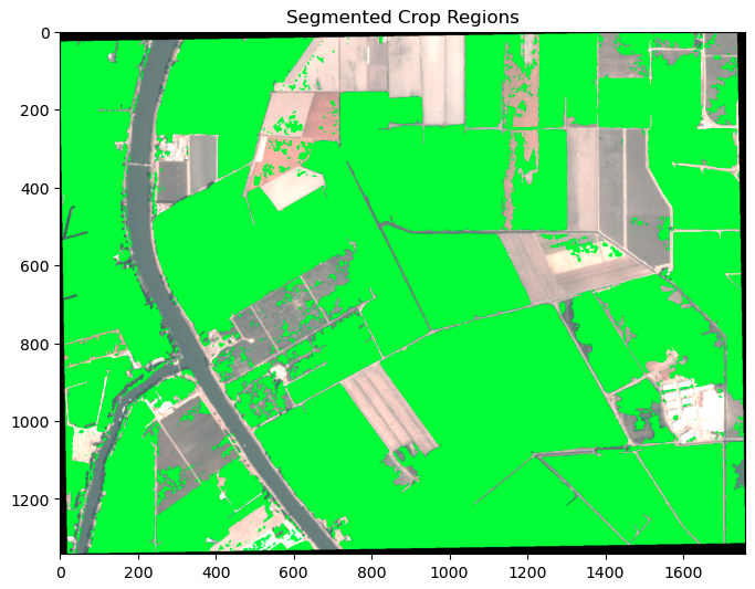
The segmented crop regions produced from the KNN classifier allow for precise identification of crop regions in the test dataset. These segmented regions can be used for various purposes, such as field boundary identification, crop monitoring, yield estimation, and resource allocation. The achieved F1 score of 0.77 is good and provides evidence that the KNN classifier is an effective tool for crop segmentation in remote sensing images. These results can be used to further improve and refine crop segmentation techniques, potentially leading to increased accuracy and efficiency in crop analysis.

Conclusion

This post demonstrated how you can use the combination of Planet’s high cadence, high-resolution satellite imagery and SageMaker geospatial capabilities to perform crop segmentation analysis, unlocking valuable insights that can improve agricultural efficiency, environmental sustainability, and food security. Accurately identifying crop regions enables further analysis on crop growth and productivity, monitoring of land use changes, and detection of potential food security risks.

Moreover, the combination of Planet data and SageMaker offers a wide range of use cases beyond crop segmentation. The insights can enable data-driven decisions on crop management, resource allocation, and policy planning in agriculture alone. With different data and ML models, the combined offering could also expand into other industries and use cases towards digital transformation, sustainability transformation, and security.

To start using SageMaker geospatial capabilities, see Get started with Amazon SageMaker geospatial capabilities.

To learn more about Planet’s imagery specifications and developer reference materials, visit Planet Developer’s Center. For documentation on Planet’s SDK for Python, see Planet SDK for Python. For more information about Planet, including its existing data products and upcoming product releases, visit https://www.planet.com/.

Planet Labs PBC Forward-Looking Statements

Except for the historical information contained herein, the matters set forth in this blog post are forward-looking statements within the meaning of the “safe harbor” provisions of the Private Securities Litigation Reform Act of 1995, including, but not limited to, Planet Labs PBC’s ability to capture market opportunity and realize any of the potential benefits from current or future product enhancements, new products, or strategic partnerships and customer collaborations. Forward-looking statements are based on Planet Labs PBC’s management’s beliefs, as well as assumptions made by, and information currently available to them. Because such statements are based on expectations as to future events and results and are not statements of fact, actual results may differ materially from those projected. Factors which may cause actual results to differ materially from current expectations include, but are not limited to the risk factors and other disclosures about Planet Labs PBC and its business included in Planet Labs PBC’s periodic reports, proxy statements, and other disclosure materials filed from time to time with the Securities and Exchange Commission (SEC) which are available online at www.sec.gov, and on Planet Labs PBC’s website at www.planet.com. All forward-looking statements reflect Planet Labs PBC’s beliefs and assumptions only as of the date such statements are made. Planet Labs PBC undertakes no obligation to update forward-looking statements to reflect future events or circumstances.

About the authors

Lydia Lihui Zhang is the Business Development Specialist at Planet Labs PBC, where she helps connect space for the betterment of earth across various sectors and a myriad of use cases. Previously, she was a data scientist at McKinsey ACRE, an agriculture-focused solution. She holds a Master of Science from MIT Technology Policy Program, focusing on space policy. Geospatial data and its broader impact on business and sustainability have been her career focus.

Mansi Shah is a software engineer, data scientist, and musician whose work explores the spaces where artistic rigor and technical curiosity collide. She believes data (like art!) imitates life, and is interested in the profoundly human stories behind the numbers and notes.

Xiong Zhou is a Senior Applied Scientist at AWS. He leads the science team for Amazon SageMaker geospatial capabilities. His current area of research includes computer vision and efficient model training. In his spare time, he enjoys running, playing basketball, and spending time with his family.

Janosch Woschitz is a Senior Solutions Architect at AWS, specializing in geospatial AI/ML. With over 15 years of experience, he supports customers globally in leveraging AI and ML for innovative solutions that capitalize on geospatial data. His expertise spans machine learning, data engineering, and scalable distributed systems, augmented by a strong background in software engineering and industry expertise in complex domains such as autonomous driving.

Shital Dhakal is a Sr. Program Manager with the SageMaker geospatial ML team based in the San Francisco Bay Area. He has a background in remote sensing and Geographic Information System (GIS). He is passionate about understanding customers pain points and building geospatial products to solve them. In his spare time, he enjoys hiking, traveling, and playing tennis.

Read More

This post is co-written with Ilan Geller and Shuyu Yang from Accenture.

Enterprises today face major challenges when it comes to using their information and knowledge bases for both internal and external business operations. With constantly evolving operations, processes, policies, and compliance requirements, it can be extremely difficult for employees and customers to stay up to date. At the same time, the unstructured nature of much of this content makes it time consuming to find answers using traditional search.

Internally, employees can often spend countless hours hunting down information they need to do their jobs, leading to frustration and reduced productivity. And when they can’t find answers, they have to escalate issues or make decisions without complete context, which can create risk.

Externally, customers can also find it frustrating to locate the information they are seeking. Although enterprise knowledge bases have, over time, improved the customer experience, they can still be cumbersome and difficult to use. Whether seeking answers to a product-related question or needing information about operating hours and locations, a poor experience can lead to frustration, or worse, a customer defection.

In either case, as knowledge management becomes more complex, generative AI presents a game-changing opportunity for enterprises to connect people to the information they need to perform and innovate. With the right strategy, these intelligent solutions can transform how knowledge is captured, organized, and used across an organization.

To help tackle this challenge, Accenture collaborated with AWS to build an innovative generative AI solution called Knowledge Assist. By using AWS generative AI services, the team has developed a system that can ingest and comprehend massive amounts of unstructured enterprise content.

Rather than traditional keyword searches, users can now ask questions and extract precise answers in a straightforward, conversational interface. Generative AI understands context and relationships within the knowledge base to deliver personalized and accurate responses. As it fields more queries, the system continuously improves its language processing through machine learning (ML) algorithms.

Since launching this AI assistance framework, companies have seen dramatic improvements in employee knowledge retention and productivity. By providing quick and precise access to information and enabling employees to self-serve, this solution reduces training time for new hires by over 50% and cuts escalations by up to 40%.

With the power of generative AI, enterprises can transform how knowledge is captured, organized, and shared across the organization. By unlocking their existing knowledge bases, companies can boost employee productivity and customer satisfaction. As Accenture’s collaboration with AWS demonstrates, the future of enterprise knowledge management lies in AI-driven systems that evolve through interactions between humans and machines.

Accenture is working with AWS to help clients deploy Amazon Bedrock, utilize the most advanced foundational models such as Amazon Titan, and deploy industry-leading technologies such as Amazon SageMaker JumpStart and Amazon Inferentia alongside other AWS ML services.

This post provides an overview of an end-to-end generative AI solution developed by Accenture for a production use case using Amazon Bedrock and other AWS services.

Solution overview

A large public health sector client serves millions of citizens every day, and they demand easy access to up-to-date information in an ever-changing health landscape. Accenture has integrated this generative AI functionality into an existing FAQ bot, allowing the chatbot to provide answers to a broader array of user questions. Increasing the ability for citizens to access pertinent information in a self-service manner saves the department time and money, lessening the need for call center agent interaction. Key features of the solution include:

• Hybrid intent approach – Uses generative and pre-trained intents
• Multi-lingual support – Converses in English and Spanish
• Conversational analysis – Reports on user needs, sentiment, and concerns
• Natural conversations – Maintains context with human-like natural language processing (NLP)
• Transparent citations – Guides users to the source information

Accenture’s generative AI solution provides the following advantages over existing or traditional chatbot frameworks:

• Generates accurate, relevant, and natural-sounding responses to user queries quickly
• Remembers the context and answers follow-up questions
• Handles queries and generates responses in multiple languages (such as English and Spanish)
• Continuously learns and improves responses based on user feedback
• Is easily integrable with your existing web platform
• Ingests a vast repository of enterprise knowledge base
• Responds in a human-like manner
• The evolution of the knowledge is continuously available with minimal to no effort
• Uses a pay-as-you-use model with no upfront costs

The high-level workflow of this solution involves the following steps:

1. Users create a simple integration with existing web platforms.​
2. Data is ingested into the platform as a bulk upload on day 0 and then incremental uploads day 1+. ​
3. User queries are processed in real time with the system scaling as required to meet user demand.
4. Conversations are saved in application databases (Amazon Dynamo DB) to support multi-round conversations.​
5. The Anthropic Claude foundation model is invoked via Amazon Bedrock, which is used to generate query responses based on the most relevant content.
6. The Anthropic Claude foundation model is used to translate queries as well as responses from English to other desired languages to support multi-language conversations.
7. The Amazon Titan foundation model is invoked via Amazon Bedrock to generate vector embeddings​.
8. Content relevance is determined through similarity of raw content embeddings and the user query embedding by using Pinecone vector database embeddings.​
9. The context along with the user’s question is appended to create a prompt, which is provided as input to the Anthropic Claude model. The generated response is provided back to the user via the web platform.

The following diagram illustrates the solution architecture.

The architecture flow can be understood in two parts:

• Offline data loading to Amazon Kendra
• End-user online flow

In the following sections, we discuss different aspects of the solution and its development in more detail.

Model selection

The process for model selection included regress testing of various models available in Amazon Bedrock, which included AI21 Labs, Cohere, Anthropic, and Amazon foundation models. We checked for supported use cases, model attributes, maximum tokens, cost, accuracy, performance, and languages. Based on this, we selected Claude-2 as best suited for this use case.

Data source

We created an Amazon Kendra index and added a data source using web crawler connectors with a root web URL and directory depth of two levels. Several webpages were ingested into the Amazon Kendra index and used as the data source.

GenAI chatbot request and response process

Steps in this process consist of an end-to-end interaction with a request from Amazon Lex and a response from a large language model (LLM):

1. The user submits the request to the conversational front-end application hosted in an Amazon Simple Storage Service (Amazon S3) bucket through Amazon Route 53 and Amazon CloudFront.
2. Amazon Lex understands the intent and directs the request to the orchestrator hosted in an AWS Lambda function.
3. The orchestrator Lambda function performs the following steps:
   1. The function interacts with the application database, which is hosted in a DynamoDB-managed database. The database stores the session ID and user ID for conversation history.
   2. Another request is sent to the Amazon Kendra index to get the top five relevant search results to build the relevant context. Using this context, modified prompt is constructed required for the LLM model.
   3. The connection is established between Amazon Bedrock and the orchestrator. A request is posted to the Amazon Bedrock Claude-2 model to get the response from the LLM model selected.
4. The data is post-processed from the LLM response and a response is sent to the user.

Online reporting

The online reporting process consists of the following steps:

1. End-users interact with the chatbot via a CloudFront CDN front-end layer.
2. Each request/response interaction is facilitated by the AWS SDK and sends network traffic to Amazon Lex (the NLP component of the bot).
3. Metadata about the request/response pairings are logged to Amazon CloudWatch.
4. The CloudWatch log group is configured with a subscription filter that sends logs into Amazon OpenSearch Service.
5. Once available in OpenSearch Service, logs can be used to generate reports and dashboards using Kibana.

Conclusion

In this post, we showcased how Accenture is using AWS generative AI services to implement an end-to-end approach towards digital transformation. We identified the gaps in traditional question answering platforms and augmented generative intelligence within its framework for faster response times and continuously improving the system while engaging with the users across the globe. Reach out to the Accenture Center of Excellence team to dive deeper into the solution and deploying this solution for your clients.

This Knowledge Assist platform can be applied to different industries, including but not limited to health sciences, financial services, manufacturing, and more. This platform provides natural, human-like responses to questions using knowledge that is secured. This platform enables efficiency, productivity, and more accurate actions for its users can take.

The joint effort builds on the 15-year strategic relationship between the companies and uses the same proven mechanisms and accelerators built by the Accenture AWS Business Group (AABG).

Connect with the AABG team at accentureaws@amazon.com to drive business outcomes by transforming to an intelligent data enterprise on AWS.

For further information about generative AI on AWS using Amazon Bedrock or Amazon SageMaker, we recommend the following resources:

• Generative AI on AWS: Technology
• Get started with generative AI on AWS using Amazon SageMaker JumpStart

You can also sign up for the AWS generative AI newsletter, which includes educational resources, blogs, and service updates.

About the Authors

Ilan Geller is the Managing Director at Accenture with focus on Artificial Intelligence, helping clients Scale Artificial Intelligence applications and the Global GenAI COE Partner Lead for AWS.

Shuyu Yang is Generative AI and Large Language Model Delivery Lead and also leads CoE (Center of Excellence) Accenture AI (AWS DevOps professional) teams.

Shikhar Kwatra is an AI/ML specialist solutions architect at Amazon Web Services, working with a leading Global System Integrator. He has earned the title of one of the Youngest Indian Master Inventors with over 500 patents in the AI/ML and IoT domains. Shikhar aids in architecting, building, and maintaining cost-efficient, scalable cloud environments for the organization, and supports the GSI partner in building strategic industry solutions on AWS.

Jay Pillai is a Principal Solution Architect at Amazon Web Services. In this role, he functions as the Global Generative AI Lead Architect and also the Lead Architect for Supply Chain Solutions with AABG. As an Information Technology Leader, Jay specializes in artificial intelligence, data integration, business intelligence, and user interface domains. He holds 23 years of extensive experience working with several clients across supply chain, legal technologies, real estate, financial services, insurance, payments, and market research business domains.

Karthik Sonti leads a global team of Solutions Architects focused on conceptualizing, building, and launching horizontal, functional, and vertical solutions with Accenture to help our joint customers transform their business in a differentiated manner on AWS.

Read More

We’re excited to announce that Amazon SageMaker Canvas now offers a quicker and more user-friendly way to create machine learning models for time-series forecasting. SageMaker Canvas is a visual point-and-click service that enables business analysts to generate accurate machine learning (ML) models without requiring any machine learning experience or having to write a single line of code.

SageMaker Canvas supports a number of use cases, including time-series forecasting used for inventory management in retail, demand planning in manufacturing, workforce and guest planning in travel and hospitality, revenue prediction in finance, and many other business-critical decisions where highly-accurate forecasts are important. As an example, time-series forecasting allows retailers to predict future sales demand and plan for inventory levels, logistics, and marketing campaigns. Time-series forecasting models in SageMaker Canvas use advanced technologies to combine statistical and machine learning algorithms, and deliver highly accurate forecasts.

In this post, we describe the enhancements to the forecasting capabilities of SageMaker Canvas and guide you on using its user interface (UI) and AutoML APIs for time-series forecasting. While the SageMaker Canvas UI offers a code-free visual interface, the APIs empower developers to interact with these features programmatically. Both can be accessed from the SageMaker console.

Improvements in forecasting experience

With today’s launch, SageMaker Canvas has upgraded its forecasting capabilities using AutoML, delivering up to 50 percent faster model building performance and up to 45 percent quicker predictions on average compared to previous versions across various benchmark datasets. This reduces the average model training duration from 186 to 73 minutes and the average prediction time from 33 to 18 minutes for a typical batch of 750 time series with data size up to 100 MB. Users can now also programmatically access model construction and prediction functions through Amazon SageMaker Autopilot APIs,  which come with model explainability and performance reports.

Previously, introducing incremental data required retraining the entire model, which was time-consuming and caused operational delays. Now, in SageMaker Canvas, you can add recent data to generate future forecasts without retraining the entire model. Just input your incremental data to your model to use the latest insights for upcoming forecasts. Eliminating retraining accelerates the forecasting process, allowing you to more quickly apply those results to your business processes.

With SageMaker Canvas now using AutoML for forecasting, you can harness model building and prediction functions through SageMaker Autopilot APIs, ensuring consistency across the UI and APIs. For example, you can start with building models in the UI, then switch to using APIs for generating predictions. This updated modeling approach also enhances model transparency in several ways:

1. Users can access an explainability report that offers clearer insights into factors influencing predictions. This is valuable for risk, compliance teams, and external regulators. The report elucidates how dataset attributes influence specific time series forecasts. It employs impact scores to measure each attribute’s relative effect, indicating whether they amplify or reduce forecast values.
2. You can now access the trained models and deploy them to SageMaker Inference or your preferred infrastructure for predictions.
3. A performance report is available, granting deeper insights into optimal models chosen by AutoML for specific time series and the hyperparameters used during training.

Generate time-series forecasts using the SageMaker Canvas UI

The SageMaker Canvas UI lets you seamlessly integrate data sources from the cloud or on-premises, merge datasets effortlessly, train precise models, and make predictions with emerging data—all without coding. Let’s explore generating a time-series forecast using this UI.

First, you import data into SageMaker Canvas from various sources, including from local files from your computer, Amazon Simple Storage Service (Amazon S3) buckets, Amazon Athena, Snowflake, and over 40 other data sources. After importing data, you can explore and visualize it to get additional insights, such as with scatterplots or bar charts. After you’re ready to create a model, you can do it with just a few clicks after configuring necessary parameters, such as selecting a target column to forecast and specifying how many days into the future you want to forecast. The following screenshots show an example visualization of predicting product demand based on historical weekly demand data for specific products in different store locations:

The following image shows weekly forecasts for a specific product in different store locations:

For a comprehensive guide on how to use the SageMaker Canvas UI for forecasting, check out this blog post.

If you need an automated workflow or direct ML model integration into apps, our forecasting functions are accessible through APIs. In the following section, we provide a sample solution detailing how to employ our APIs for automated forecasting.

Generate time-series forecast using APIs

Let’s dive into how to use the APIs to train the model and generate predictions. For this demonstration, consider a situation where a company needs to predict product stock levels at various stores to meet customer demand. At a high level, the API interactions break down into the following steps:

1. Prepare the dataset.
2. Create a SageMaker Autopilot job.
3. Evaluate the Autopilot job:
   1. Explore the model accuracy metrics and backtest results.
   2. Explore the model explainability report.
4. Generate predictions from the model:
   1. Use the real-time inference endpoint created as part of the Autopilot job; or
   2. Use a batch transform job.

Sample Amazon SageMaker Studio notebook showcasing forecasting with APIs

We’ve provided a sample SageMaker Studio notebook on GitHub to help accelerate your time-to-market when your business prefers to orchestrate forecasting through programmatic APIs. The notebook offers a sample synthetic dataset available through a public S3 bucket. The notebook guides you through all the steps outlined in the workflow image mentioned above. While the notebook provides a basic framework, you can tailor the code sample to fit your specific use case. This includes modifying it to match your unique data schema, time-resolution, forecasting horizon, and other necessary parameters to achieve your desired results.

Conclusion

SageMaker Canvas democratizes time-series forecasting by offering a user-friendly, code-free experience that empowers business analysts to create highly accurate machine learning models. With today’s AutoML upgrades, it delivers up to 50 percent faster model building, up to 45 percent quicker predictions, and introduces API access for both model construction and prediction functions, enhancing its transparency and consistency. The unique ability of SageMaker Canvas to seamlessly handle incremental data without retraining ensures swift adaptation to ever-changing business demands.

Whether you prefer the intuitive UI or versatile APIs, SageMaker Canvas simplifies data integration, model training, and prediction, making it a pivotal tool for data-driven decision-making and innovation across industries.

To learn more, review the documentation, or explore the notebook available in our GitHub repository. Pricing information for time-series forecasting using SageMaker Canvas is available on the SageMaker Canvas Pricing page, and for SageMaker training and inference pricing when using SageMaker Autopilot APIs please see the SageMaker Pricing page.

These capabilities are available in all AWS Regions where SageMaker Canvas and SageMaker Autopilot are publicly accessible. For more information about Region availability, see AWS Services by Region.

About the Authors

Nirmal Kumar is Sr. Product Manager for the Amazon SageMaker service. Committed to broadening access to AI/ML, he steers the development of no-code and low-code ML solutions. Outside work, he enjoys travelling and reading non-fiction.

Charles Laughlin is a Principal AI/ML Specialist Solution Architect who works on the Amazon SageMaker service team at AWS. He helps shape the service roadmap and collaborates daily with diverse AWS customers to help transform their businesses using cutting-edge AWS technologies and thought leadership. Charles holds a M.S. in Supply Chain Management and a Ph.D. in Data Science.

Ridhim Rastogi a Software Development Engineer who works on Amazon SageMaker service team at AWS. He is passionate about building scalable distributed systems with a focus on solving real-world problems through AI/ML. In his spare time, he likes to solve puzzles, read fiction, and explore his surroundings.

Ahmed Raafat is a Principal Solutions Architect at AWS, with 20 years of field experience and a dedicated focus of 5 years within the AWS ecosystem. He specializes in AI/ML solutions. His extensive experience extends across various industry verticals, rendering him a trusted advisor for numerous enterprise customers, facilitating their seamless navigation and acceleration of their cloud journey.

John Oshodi is a Senior Solutions Architect at Amazon Web Services based in London, UK. He specializes in data and analytics and serves as a technical advisor for numerous AWS enterprise customers, supporting and accelerating their cloud journey. Outside of work, he enjoys travelling to new places and experiencing new cultures with his family.

Read More

In the world of data-driven decision-making, time series forecasting is key in enabling businesses to use historical data patterns to anticipate future outcomes. Whether you are working in asset risk management, trading, weather prediction, energy demand forecasting, vital sign monitoring, or traffic analysis, the ability to forecast accurately is crucial for success.

In these applications, time series data can have heavy-tailed distributions, where the tails represent extreme values. Accurate forecasting in these regions is important in determining how likely an extreme event is and whether to raise an alarm. However, these outliers significantly impact the estimation of the base distribution, making robust forecasting challenging. Financial institutions rely on robust models to predict outliers such as market crashes. In energy, weather, and healthcare sectors, accurate forecasts of infrequent but high-impact events such as natural disasters and pandemics enable effective planning and resource allocation. Neglecting tail behavior can lead to losses, missed opportunities, and compromised safety. Prioritizing accuracy at the tails helps lead to reliable and actionable forecasts. In this post, we train a robust time series forecasting model capable of capturing such extreme events using Amazon SageMaker.

To effectively train this model, we establish an MLOps infrastructure to streamline the model development process by automating data preprocessing, feature engineering, hyperparameter tuning, and model selection. This automation reduces human error, improves reproducibility, and accelerates the model development cycle. With a training pipeline, businesses can efficiently incorporate new data and adapt their models to evolving conditions, which helps ensure that forecasts remain reliable and up to date.

After the time series forecasting model is trained, deploying it within an endpoint grants real-time prediction capabilities. This empowers you to make well-informed and responsive decisions based on the most recent data. Furthermore, deploying the model in an endpoint enables scalability, because multiple users and applications can access and utilize the model simultaneously. By following these steps, businesses can harness the power of robust time series forecasting to make informed decisions and stay ahead in a rapidly changing environment.

Overview of solution

This solution showcases the training of a time series forecasting model, specifically designed to handle outliers and variability in data using a Temporal Convolutional Network (TCN) with a Spliced Binned Pareto (SBP) distribution. For more information about a multimodal version of this solution, refer to The science behind NFL Next Gen Stats’ new passing metric. To further illustrate the effectiveness of the SBP distribution, we compare it with the same TCN model but using a Gaussian distribution instead.

This process significantly benefits from the MLOps features of SageMaker, which streamline the data science workflow by harnessing the powerful cloud infrastructure of AWS. In our solution, we use Amazon SageMaker Automatic Model Tuning for hyperparameter search, Amazon SageMaker Experiments for managing experiments, Amazon SageMaker Model Registry to manage model versions, and Amazon SageMaker Pipelines to orchestrate the process. We then deploy our model to a SageMaker endpoint to obtain real-time predictions.

The following diagram illustrates the architecture of the training pipeline.

The following diagram illustrates the inference pipeline.

You can find the complete code in the GitHub repo. To implement the solution, run the cells in SBP_main.ipynb.

Click here to open the AWS console and follow along.

SageMaker pipeline

SageMaker Pipelines offers a user-friendly Python SDK to create integrated machine learning (ML) workflows. These workflows, represented as Directed Acyclic Graphs (DAGs), consist of steps with various types and dependencies. With SageMaker Pipelines, you can streamline the end-to-end process of training and evaluating models, enhancing efficiency and reproducibility in your ML workflows.

The training pipeline begins with generating a synthetic dataset that is split into training, validation, and test sets. The training set is used to train two TCN models, one utilizing Spliced Binned-Pareto distribution and the other employing Gaussian distribution. Both models go through hyperparameter tuning using the validation set to optimize each model. Afterward, an evaluation against the test set is conducted to determine the model with the lowest root mean squared error (RMSE). The model with the best accuracy metric is uploaded to the model registry.

The following diagram illustrates the pipeline steps.

Let’s discuss the steps in more detail.

Data generation

The first step in our pipeline generates a synthetic dataset, which is characterized by a sinusoidal waveform and asymmetric heavy-tailed noise. The data was created using a number of parameters, such as degrees of freedom, a noise multiplier, and a scale parameter. These elements influence the shape of the data distribution, modulate the random variability in our data, and adjust the spread of our data distribution, respectively.

This data processing job is accomplished using a PyTorchProcessor, which runs PyTorch code (generate_data.py) within a container managed by SageMaker. Data and other relevant artifacts for debugging are located in the default Amazon Simple Storage Service (Amazon S3) bucket associated with the SageMaker account. Logs for each step in the pipeline can be found in Amazon CloudWatch.

The following figure is a sample of the data generated by the pipeline.

You can replace the input with a wide variety of time series data, such as symmetric, asymmetric, light-tailed, heavy-tailed, or multimodal distribution. The model’s robustness allows it to be applicable to a broad range of time series problems, provided sufficient observations are available.

Model training

After data generation, we train two TCNs: one using SBP distribution and other using Gaussian distribution. SBP distribution employs a discrete binned distribution as its predictive base, where the real axis is divided into discrete bins, and the model predicts the likelihood of an observation falling within each bin. This methodology enables the capture of asymmetries and multiple modes because the probability of each bin is independent. An example of the binned distribution is shown in the following figure.

The predictive binned distribution on the left is robust to extreme events because the log-likelihood is not dependent on the distance between the predicted mean and observed point, differing from parametric distributions like Gaussian or Student’s t. Therefore, the extreme event represented by the red dot will not bias the learned mean of the distribution. However, the extreme event will have zero probability. To capture extreme events, we form an SBP distribution by defining the lower tail at the 5th quantile and the upper tail at the 95th quantile, replacing both tails with weighted Generalized Pareto Distributions (GPD), which can quantify the likeliness of the event. The TCN will output the parameters for the binned distribution base and GPD tails.

Hyperparameter search

For optimal output, we use automatic model tuning to find the best version of a model through hyperparameter tuning. This step is integrated into SageMaker Pipelines and allows for the parallel run of multiple training jobs, employing various methods and predefined hyperparameter ranges. The result is the selection of the best model based on the specified model metric, which is RMSE. In our pipeline, we specifically tune the learning rate and number of training epochs to optimize our model’s performance. With the hyperparameter tuning capability in SageMaker, we increase the likelihood that our model achieves optimal accuracy and generalization for the given task.

Due to the synthetic nature of our data, we are keeping Context Length and Lead Time as static parameters. Context Length refers to the number of historical time steps inputted into the model, and Lead Time represents the number of time steps in our forecast horizon. For the sample code, we are only tuning Learning Rate and the number of epochs to save on time and cost.

SBP-specific parameters are kept constant based on extensive testing by the authors on the original paper across different datasets:

• Number of Bins (100) – This parameter determines the number of bins used to model the base of the distribution. It is kept at 100, which has proven to be most effective across multiple industries.
• Percentile Tail (0.05) – This denotes the size of the generalized Pareto distributions at the tail. Like the previous parameter, this has been exhaustively tested and found to be most efficient.

Experiments

The hyperparameter process is integrated with SageMaker Experiments, which helps organize, analyze, and compare iterative ML experiments, providing insights and facilitating tracking of the best-performing models. Machine learning is an iterative process involving numerous experiments encompassing data variations, algorithm choices, and hyperparameter tuning. These experiments serve to incrementally refine model accuracy. However, the large number of training runs and model iterations can make it challenging to identify the best-performing models and make meaningful comparisons between current and past experiments. SageMaker Experiments addresses this by automatically tracking our hyperparameter tuning jobs and allowing us to gain further details and insight into the tuning process, as shown in the following screenshot.

Model evaluation

The models undergo training and hyperparameter tuning, and are subsequently evaluated via the evaluate.py script. This step utilizes the test set, distinct from the hyperparameter tuning stage, to gauge the model’s real-world accuracy. RMSE is used to assess the accuracy of the predictions.

For distribution comparison, we employ a probability-probability (P-P) plot, which assesses the fit between the actual vs. predicted distributions. The closeness of the points to the diagonal indicates a perfect fit. Our comparisons between SBP’s and Gaussian’s predicted distributions against the actual distribution show that SBP’s predictions align more closely with the actual data.

As we can observe, SBP has lower RMSE on the base, lower tail, and upper tail. The SBP distribution improved the accuracy of the Gaussian distribution by 61% on the base, 56% on the lower tail, and 30% on the upper tail. Overall, the SBP distribution has significantly better results.

Model selection

We use a condition step in SageMaker Pipelines to analyze model evaluation reports, opting for the model with the lowest RMSE for improved distribution accuracy. The selected model is converted into a SageMaker model object, readying it for deployment. This involves creating a model package with crucial parameters and packaging it into a ModelStep.

Model registry

The selected model is then uploaded to SageMaker Model Registry, which plays a critical role in managing models ready for production. It stores models, organizes model versions, captures essential metadata and artifacts such as container images, and governs the approval status of each model. By using the registry, we can efficiently deploy models to accessible SageMaker environments and establish a foundation for continuous integration and continuous deployment (CI/CD) pipelines.

Inference

Upon completion of our training pipeline, our model is then deployed using SageMaker hosting services, which enables the creation of an inference endpoint for real-time predictions. This endpoint allows seamless integration with applications and systems, providing on-demand access to the model’s predictive capabilities through a secure HTTPS interface. Real-time predictions can be used in scenarios such as stock price and energy demand forecast. Our endpoint provides a single-step forecast for the provided time series data, presented as percentiles and the median, as shown in the following figure and table.

Clean up

After you run this solution, make sure you clean up any unnecessary AWS resources to avoid unexpected costs. You can clean up these resources using the SageMaker Python SDK, which can be found at the end of the notebook. By deleting these resources, you prevent further charges for resources you are no longer using.

Conclusion

Having an accurate forecast can highly impact a business’s future planning and can also provide solutions to a variety of problems in different industries. Our exploration of robust time series forecasting with MLOps on SageMaker has demonstrated a method to obtain an accurate forecast and the efficiency of a streamlined training pipeline.

Our model, powered by a Temporal Convolutional Network with Spliced Binned Pareto distribution, has shown accuracy and adaptability to outliers by improving the RMSE by 61% on the base, 56% on the lower tail, and 30% on the upper tail over the same TCN with Gaussian distribution. These figures make it a reliable solution for real-world forecasting needs.

The pipeline demonstrates the value of automating MLOps features. This can reduce manual human effort, enable reproducibility, and accelerate model deployment. SageMaker features such as SageMaker Pipelines, automatic model tuning, SageMaker Experiments, SageMaker Model Registry, and endpoints make this possible.

Our solution employs a miniature TCN, optimizing just a few hyperparameters with a limited number of layers, which are sufficient for effectively highlighting the model’s performance. For more complex use cases, consider using PyTorch or other PyTorch-based libraries to construct a more customized TCN that aligns with your specific needs. Additionally, it would be beneficial to explore other SageMaker features to enhance your pipeline’s functionality further. To fully automate the deployment process, you can use the AWS Cloud Development Kit (AWS CDK) or AWS CloudFormation.

For more information on time series forecasting on AWS, refer to the following:

• Amazon Forecast
• Deep demand forecasting with Amazon SageMaker
• Hierarchical Forecasting using Amazon SageMaker
• Build a cold start time series forecasting engine using AutoGluon

Feel free to leave a comment with any thoughts or questions!

About the Authors

Nick Biso is a Machine Learning Engineer at AWS Professional Services. He solves complex organizational and technical challenges using data science and engineering. In addition, he builds and deploys AI/ML models on the AWS Cloud. His passion extends to his proclivity for travel and diverse cultural experiences.

Alston Chan is a Software Development Engineer at Amazon Ads. He builds machine learning pipelines and recommendation systems for product recommendations on the Detail Page. Outside of work, he enjoys game development and rock climbing.

Maria Masood specializes in building data pipelines and data visualizations at AWS Commerce Platform. She has expertise in Machine Learning, covering natural language processing, computer vision, and time-series analysis. A sustainability enthusiast at heart, Maria enjoys gardening and playing with her dog during her downtime.

Read More

In the rapidly evolving world of AI and machine learning (ML), foundation models (FMs) have shown tremendous potential for driving innovation and unlocking new use cases. However, as organizations increasingly harness the power of FMs, concerns surrounding data privacy, security, added cost, and compliance have become paramount. Regulated and compliance-oriented industries, such as financial services, healthcare and life sciences, and government institutes, face unique challenges in ensuring the secure and responsible consumption of these models. To strike a balance between agility, innovation, and adherence to standards, a robust platform becomes essential. In this post, we propose Generative AI Gateway as platform for an enterprise to allow secure access to FMs for rapid innovation.

In this post, we define what a Generative AI Gateway is, its benefits, and how to architect one on AWS. A Generative AI Gateway can help large enterprises control, standardize, and govern FM consumption from services such as Amazon Bedrock, Amazon SageMaker JumpStart, third-party model providers (such as Anthropic and their APIs), and other model providers outside of the AWS ecosystem.

What is a Generative AI Gateway?

For traditional APIs (such as REST or gRPC), API Gateway has established itself as a design pattern that enables enterprises to standardize and control how APIs are externalized and consumed. In addition, API Registries enabled centralized governance, control, and discoverability of APIs.

Similarly, Generative AI Gateway is a design pattern that aims to expand on API Gateway and Registry patterns with considerations specific to serving and consuming foundation models in large enterprise settings. For example, handling hallucinations, managing company-specific IPs and EULAs (End User License Agreements), as well as moderating generations are new responsibilities that go beyond the scope of traditional API Gateways.

In addition to requirements specific for generative AI, the technological and regulatory landscape for foundation models is changing fast. This creates unique challenges for organizations to balance innovation speed and compliance. For example:

• The state-of-the-art (SOTA) of models, architectures, and best practices are constantly changing. This means companies need loose coupling between app clients (model consumers) and model inference endpoints, which ensures easy switch among large language model (LLM), vision, or multi-modal endpoints if needed. An abstraction layer over model inference endpoints provides such loose coupling.
• Regulatory uncertainty, especially over IP and data privacy, requires observability, monitoring, and trace of generations. For example, if Retrieval Augmented Generation (RAG)-based applications accidentally include personally identifiable information (PII) data in context, such issues need to be detected in real time. This becomes challenging if large enterprises with multiple data science teams use bespoke, distributed platforms for deploying foundation models.

Generative AI Gateway aims to solve for these new requirements while providing the same benefits of traditional API Gateways and Registries, such as centralized governance and observability, and reuse of common components.

Solution overview

Specifically, Generative AI Gateway provides the following key components:

• A model abstraction layer for approved FMs
• An API Gateway for FMs (AI Gateway)
• A playground for FMs for internal model discoverability

The following diagram illustrates the solution architecture.

For added resilience, the suggested solution can be deployed in a Multi-AZ environment. The dotted lines in the preceding diagram represent network boundaries, although the entire solution can be deployed in a single VPC.

Model abstraction layer

The model abstraction layer serves as the foundation for secure and controlled access to the organization’s pool of FMs. The layer serves a single source of truth on which models are available to the company, team, and employee, as well as how to access each model by storing endpoint information for each model.

This layer serves as the cornerstone for secure, compliant, and agile consumption of FMs through the Generative AI Gateway, promoting responsible AI practices within the organization.

The layer itself consists of four main components:

• FM endpoint registry – After the FMs are evaluated, approved, and deployed for usage, their endpoints are added to the FM endpoint registry—a centralized repository of all deployed or externally accessible API endpoints. The registry contains metadata about generative AI service endpoints that an organization consumes, whether it’s an internally deployed FM or an externally provided generative AI API from a vendor. The metadata includes information such as service endpoint information for each foundation model and their configuration, and access policies (based on role, team, and so on).
• Model policy store and engine – For FMs to be consumed in a compliant manner, the model abstraction layer must track qualitative and quantitative rules for model generations. For example, some generations might be subject to certain regulations such as CCPA (California Consumer Privacy Act), which requires custom generation behavior per geo. Therefore, the policies should be country and geo aware, to ensure compliance across changing regulatory environments across locales.
• Identity layer – After the models are available to be consumed, the identity layer plays a pivotal role in access management, ensuring that only authorized users or roles within the organization can interact with specific FMs through the AI Gateway. Role-based access control (RBAC) mechanisms help define granular access permissions, ensuring that users can access models based on their roles and responsibilities.
• Integration with vendor model registries – FMS can be available in different ways, either deployed in organization accounts under VPCs or available as APIs through different vendors. After passing the initial checks mentioned earlier, the endpoint registry holds the necessary information about these models from vendors and their versions exposed via APIs. This abstracts way the underlying complexities from the end-user.

To populate the AI model endpoint registry, the Generative AI Gateway team collaborates with a cross-function team of domain experts and business line stakeholders to carefully select and onboard FMs to the platform. During this onboarding phase, factors like model performance, cost, ethical alignment, compliance with industry regulations, and the vendor’s reputation are carefully considered. By conducting thorough evaluations, organizations ensure that the selected FMs align with their specific business needs and adhere to security and privacy requirements.

The following diagram illustrates the architecture of this layer.

AWS services can help in building a model abstraction layer (MAL) as follows:

1. The generative AI manager creates a registry table using Amazon DynamoDB. This table is populated with information about the FMs either deployed internally in the organization account or accessible via an API from vendors. This table will hold the endpoint, metadata, and configuration parameters for the model. It can also store the information if a custom AWS Lambda function is needed to invoke the underlying FM with vendor-specific API clients.
2. The generative AI manager then determines access for the user, adds limits, adds a policy for what type of generations the user can perform (images, text, multi-modality, and so on), and adds other organization specific policies such as responsible AI and content filters that will be added as a separate policy table in DynamoDB.
3. When the user makes a request using the AI Gateway, it’s routed to Amazon Cognito to determine access for the client. A Lambda authorizer helps determine the access from the identity layer, which will be managed by the DynamoDB table policy. If the client has access, the relevant access such as the AWS Identity and Access Management (IAM) role or API key for the FM endpoint are fetched from AWS Secrets Manager. Also, the registry is explored to find the relevant endpoint and configuration at this stage.
4. After all the necessary information related to the request is fetched, such as the endpoint, configuration, access keys, and custom function, it’s handed back to the AI Gateway to be used with the dispatcher Lambda function that calls a specific model endpoint.

AI Gateway

The AI Gateway serves as a crucial component that facilitates secure and efficient consumption of FMs within the organization. It operates on top of the model abstraction layer, providing an API-based interface to internal users, including developers, data scientists, and business analysts.

Through this user-friendly interface (programmatic and playground UI-based), internal users can seamlessly access, interact with, and use the organization’s curated models, ensuring relevant models are made available based on their identities and responsibilities. An AI Gateway can comprise the following:

• A unified API interface across all FMs – The AI Gateway presents a unified API interface and SDK that abstracts the underlying technical complexities, enabling internal users to interact with the organization’s pool of FMs effortlessly. Users can use the APIs to invoke different models and send in their prompts to get model generation.
• API quota, limits, and usage management – This includes the following:
  • Consumed quota – To enable efficient resource allocation and cost control, the AI Gateway provides users with insights into their consumed quota for each model. This transparency allows users to manage their AI resource usage effectively, ensuring optimal utilization and preventing resource waste.
  • Request for dedicated hosting – Recognizing the importance of resource allocation for critical use cases, the AI Gateway allows users to request dedicated hosting of specific models. Users with high-priority or latency-sensitive applications can use this feature to ensure a consistent and dedicated environment for their model inference needs.
• Access control and model governance – Using the identity layer from the model abstraction layer, the AI Gateway enforces stringent access controls. Each user’s identity and assigned roles determine the models they can access. This granular access control ensures that users are presented with only the models relevant to their domains, maintaining data security and privacy while promoting responsible AI usage.
• Content, privacy, and responsible AI policy enforcement – The API Gateway employs both the preprocessing and postprocessing of all inputs to the model as well as the model generations to filter and moderate for toxicity, violence, harmfulness, PII data, and more that are specified by the model abstraction layer for filtering. Centralizing this function in the AI Gateway ensures enforcement and easy audit.

By integrating the AI Gateway with the model abstraction layer and incorporating features such as identity-based access control, model listing and metadata display, consumed quota monitoring, and dedicated hosting requests, organizations can create a powerful AI consumption platform.

In addition, the AI Gateway provides the standard benefits of API Gateways, such as the following:

• Cost control mechanism – To optimize resource allocation and manage costs effectively, a robust cost control mechanism can be implemented. This mechanism monitors resource usage, model inference costs, and data transfer expenses. It allows organizations to gain insights into generative AI resource expenditure, identify cost-saving opportunities, and make informed decisions on resource allocation.
• Cache – Inference from FMs can become expensive, especially during testing and development phases of the application. A cache layer can help reduce that cost and even improve the speed by maintaining a cache for frequent requests. The cache also offloads the inference burden on the endpoint, which makes room for other requests.
• Observability – This plays a crucial role in capturing activities performed on the AI Gateway and the Discovery Playground. Detailed logs record user interactions, model requests, and system responses. These logs provide valuable information for troubleshooting, tracking user behavior, and reinforcing transparency and accountability.
• Quotas, rate limits, and throttling – The governance aspect of this layer can incorporate the application of quotas, rate limits, and throttling to manage and control AI resource usage. Quotas define the maximum number of requests a user or team can make within a specific time frame, ensuring fair resource distribution. Rate limits prevent excessive usage of resources by enforcing a maximum request rate. Throttling mitigates the risk of system overload by controlling the frequency of incoming requests, preventing service disruptions.
• Audit trails and usage monitoring – The team assumes responsibility of maintaining detailed audit trails of the entire ecosystem. These logs enable comprehensive usage monitoring, allowing the central team to track user activities, identify potential risks, and maintain transparency in AI consumption.

The following diagram illustrates this architecture.

AWS services can help in building an AI Gateway as follows:

1. The user makes the request using Amazon API Gateway, which is routed to the model abstraction layer after the request has been authenticated and authorized.
2. The AI Gateway enforces usage limits for each user’s request using usage limit policies returned by the MAL. For easy enforcement, we use the native capability of API Gateway to enforce metering. In addition, we perform standard API Gateway validations on request using a JSON schema.
3. After the usage limits are validated, both the endpoint configuration and credentials received from the MAL form the actual inference payload using native interfaces provided by each of the approved model vendors. The dispatch layer normalizes the differences across vendors’ SDKs and API interfaces to provide a unified interface to the client. Issues such as DNS changes, load balancing, and caching could also be handled by a more sophisticated dispatch service.
4. After the response is received from the underlying model endpoints, postprocessing Lambda functions use the policies from the MAL pertaining to content (toxicity, nudity, and so on) as well as compliance (CCPA, GDPR, and so on) to filter or mask generations as a whole or in part.
5. Throughout the lifecycle of the request, all generations and inference payloads are logged through Amazon CloudWatch Logs, which can be organized via log groups depending on tags as well as policies retrieved from MAL. For example, logs can be separated per model vendor and geo. This allows for further model improvement and troubleshooting.
6. Finally, a retroactive audit is available through AWS CloudTrail.

Discovery Playground

The last component is to introduce a Discovery Playground, which presents a user-friendly interface built on top of the model abstraction layer and the AI Gateway, offering a dynamic environment for users to explore, test, and unleash the full potential of available FMs. Beyond providing access to AI capabilities, the playground empowers users to interact with models using a rich UI interface, provide valuable feedback, and share their discoveries with other users within the organization. It offers the following key features:

• Playground interface – You can effortlessly input prompts and receive model outputs in real time. The UI streamlines the interaction process, making generative AI exploration accessible to users with varying levels of technical expertise.
• Model cards – You can access a comprehensive list of available models along with their corresponding metadata. You can explore detailed information about each model, such as its capabilities, performance metrics, and supported use cases. This feature facilitates informed decision-making, empowering you to select the most suitable model for your specific needs.
• Feedback mechanism – A differentiating aspect of the playground would be its feedback mechanism, allowing you to provide insights on model outputs. You can report issues like hallucination (fabricated information), inappropriate language, or any unintended behavior observed during interactions with the models.
• Recommendations for use cases – The Discovery Playground can be designed to facilitate learning and understanding of FMs’ capabilities for different use cases. You can experiment with various prompts and discover which models excel in specific scenarios.

By offering a rich UI interface, model cards, feedback mechanism, use case recommendations, and the optional Example Store, the Discovery Playground becomes a powerful platform for generative AI exploration and knowledge sharing within the organization.

Process considerations

Whereas the previous modules of the Generative AI Gateway offer a platform, this layer is more practical, ensuring the responsible and compliant consumption of FMs within the organization. It encompasses additional measures that go beyond the technical aspects, focusing on legal, practical, and regulatory considerations. This layer presents crucial responsibilities for the central team to address data security, licenses, organizational regulations, and audit trails, fostering a culture of trust and transparency:

• Data security and privacy – Because FMs can process vast amounts of data, data security and privacy become paramount concerns. The central team is responsible for implementing robust data security measures, including encryption, access controls, and data anonymization. Compliance with data protection regulations, such as GDPR, HIPAA, or other industry-specific standards, is diligently ensured to safeguard sensitive information and user privacy.
• Data monitoring – A comprehensive data monitoring system should be established to track incoming and outgoing information through the AI Gateway and Discovery Playground. This includes monitoring the prompts provided by users and the corresponding model outputs. The data monitoring mechanism enables the organization to observe data patterns, detect anomalies, and ensure that sensitive information remains secure.
• Model licenses and agreements – The central team should take the lead in managing licenses and agreements associated with the use of models. Vendor-provided models may come with specific usage agreements, usage restrictions, or licensing terms. The team ensures compliance with these agreements and maintains a comprehensive repository of all licenses, ensuring a clear understanding of the rights and limitations pertaining to each model.
• Ethical considerations – As AI systems become increasingly sophisticated, the central team assumes the responsibility of ensuring ethical alignment in AI usage. They assess models for potential biases, harmful outputs, or unethical behavior. Steps are taken to mitigate such issues and foster responsible AI development and deployment within the organization.
• Proactive adaptation – To stay ahead of emerging challenges and ever-changing regulations, the central team takes a proactive approach to governance. They continuously update policies, model standards, and compliance measures to align with the latest industry practices and legal requirements. This ensures the organization’s AI ecosystem remains in compliance and upholds ethical standards.

Conclusion

The Generative AI Gateway enables organizations to use foundation models responsibly and securely. Through the integration of the model abstraction layer, AI Gateway, and Discovery Playground powered with monitoring, observability, governance, and security, compliance, and audit layers, organizations can strike a balance between innovation and compliance. The AI Gateway empowers you with seamless access to curated models, while the Discovery Playground fosters exploration and feedback. Monitoring and governance provide insights for optimized resource allocation and proactive decision-making. With a focus on security, compliance, and ethical AI practices, the Generative AI Gateway opens doors to a future where AI-driven applications thrive responsibly, unlocking new realms of possibilities for organizations.

About the Authors

Talha Chattha is an AI/ML Specialist Solutions Architect at Amazon Web Services, based in Stockholm, serving Nordic enterprises and digital native businesses. Talha holds a deep passion for Generative AI technologies, He works tirelessly to deliver innovative, scalable and valuable ML solutions in the space of Large Language Models and Foundation Models for his customers. When not shaping the future of AI, he explores the scenic European landscapes and delicious cuisines.

John Hwang is a Generative AI Architect at AWS with special focus on Large Language Model (LLM) applications, vector databases, and generative AI product strategy. He is passionate about helping companies with AI/ML product development, and the future of LLM agents and co-pilots. Prior to joining AWS, he was a Product Manager at Alexa, where he helped bring conversational AI to mobile devices, as well as a derivatives trader at Morgan Stanley. He holds a B.S. in Computer Science from Stanford University.

Paolo Di Francesco is a Senior Solutions Architect at Amazon Web Services (AWS). He holds a PhD in Telecommunication Engineering and has experience in software engineering. He is passionate about machine learning and is currently focusing on using his experience to help customers reach their goals on AWS, in particular in discussions around MLOps. Outside of work, he enjoys playing football and reading.

Read More