Monthly Archives: July 2023

Drug development is a complex and long process that involves screening thousands of drug candidates and using computational or experimental methods to evaluate leads. According to McKinsey, a single drug can take 10 years and cost an average of $2.6 billion to go through disease target identification, drug screening, drug-target validation, and eventual commercial launch. Drug discovery is the research component of this pipeline that generates candidate drugs with the highest likelihood of being effective with the least harm to patients. Machine learning (ML) methods can help identify suitable compounds at each stage in the drug discovery process, resulting in more streamlined drug prioritization and testing, saving billions in drug development costs (for more information, refer to AI in biopharma research: A time to focus and scale).

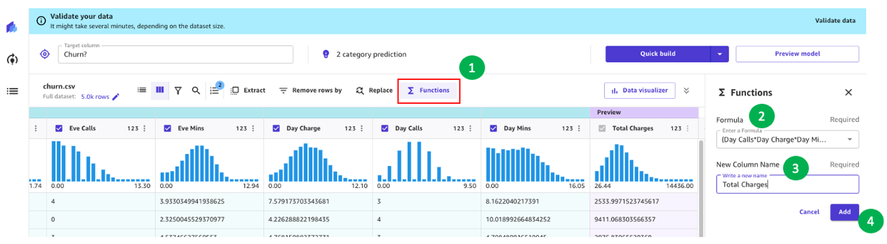
Drug targets are typically biological entities called proteins, the building blocks of life. The 3D structure of a protein determines how it interacts with a drug compound; therefore, understanding the protein 3D structure can add significant improvements to the drug development process by screening for drug compounds that fit the target protein structure better. Another area where protein structure prediction can be useful is understanding the diversity of proteins, so that we only select for drugs that selectively target specific proteins without affecting other proteins in the body (for more information, refer to Improving target assessment in biomedical research: the GOT-IT recommendations). Precise 3D structures of target proteins can enable drug design with higher specificity and lower likelihood of cross-interactions with other proteins.

However, predicting how proteins fold into their 3D structure is a difficult problem, and traditional experimental methods such as X-ray crystallography and NMR spectroscopy can be time-consuming and expensive. Recent advances in deep learning methods for protein research have shown promise in using neural networks to predict protein folding with remarkable accuracy. Folding algorithms like AlphaFold2, ESMFold, OpenFold, and RoseTTAFold can be used to quickly build accurate models of protein structures. Unfortunately, these models are computationally expensive to run and the results can be cumbersome to compare at the scale of thousands of candidate protein structures. A scalable solution for using these various tools will allow researchers and commercial R&D teams to quickly incorporate the latest advances in protein structure prediction, manage their experimentation processes, and collaborate with research partners.

Amazon SageMaker is a fully managed service to prepare, build, train, and deploy high-quality ML models quickly by bringing together a broad set of capabilities purpose-built for ML. It offers a fully managed environment for ML, abstracting away the infrastructure, data management, and scalability requirements so you can focus on building, training, and testing your models.

In this post, we present a fully managed ML solution with SageMaker that simplifies the operation of protein folding structure prediction workflows. We first discuss the solution at the high level and its user experience. Next, we walk you through how to easily set up compute-optimized workflows of AlphaFold2 and OpenFold with SageMaker. Finally, we demonstrate how you can track and compare protein structure predictions as part of a typical analysis. The code for this solution is available in the following GitHub repository.

Solution overview

In this solution, scientists can interactively launch protein folding experiments, analyze the 3D structure, monitor the job progress, and track the experiments in Amazon SageMaker Studio.

The following screenshot shows a single run of a protein folding workflow with Amazon SageMaker Studio. It includes the visualization of the 3D structure in a notebook, run status of the SageMaker jobs in the workflow, and links to the input parameters and output data and logs.

The following diagram illustrates the high-level solution architecture.

To understand the architecture, we first define the key components of a protein folding experiment as follows:

• FASTA target sequence file – The FASTA format is a text-based format for representing either nucleotide sequences or amino acid (protein) sequences, in which nucleotides or amino acids are represented using single-letter codes.
• Genetic databases – A genetic database is one or more sets of genetic data stored together with software to enable users to retrieve genetic data. Several genetic databases are required to run AlphaFold and OpenFold algorithms, such as BFD, MGnify, PDB70, PDB, PDB seqres, UniRef30 (FKA UniClust30), UniProt, and UniRef90.
• Multiple sequence alignment (MSA) – A sequence alignment is a way of arranging the primary sequences of a protein to identify regions of similarity that may be a consequence of functional, structural, or evolutionary relationships between the sequences. The input features for predictions include MSA data.
• Protein structure prediction – The structure of input target sequences is predicted with folding algorithms like AlphaFold2 and OpenFold that use a multitrack transformer architecture trained on known protein templates.
• Visualization and metrics – Visualize the 3D structure with the py3Dmol library as an interactive 3D visualization. You can use metrics to evaluate and compare structure predictions, most notably root-mean-square deviation (RMSD) and template modeling Score (TM-score)

The workflow contains the following steps:

1. Scientists use the web-based SageMaker ML IDE to explore the code base, build protein sequence analysis workflows in SageMaker Studio notebooks, and run protein folding pipelines via the graphical user interface in SageMaker Studio or the SageMaker SDK.
2. Genetic and structure databases required by AlphaFold and OpenFold are downloaded prior to pipeline setup using Amazon SageMaker Processing, an ephemeral compute feature for ML data processing, to an Amazon Simple Storage Service (Amazon S3) bucket. With SageMaker Processing, you can run a long-running job with a proper compute without setting up any compute cluster and storage and without needing to shut down the cluster. Data is automatically saved to a specified S3 bucket location.
3. An Amazon FSx for Lustre file system is set up, with the data repository being the S3 bucket location where the databases are saved. FSx for Lustre can scale to hundreds of GB/s of throughput and millions of IOPS with low-latency file retrieval. When starting an estimator job, SageMaker mounts the FSx for Lustre file system to the instance file system, then starts the script.
4. Amazon SageMaker Pipelines is used to orchestrate multiple runs of protein folding algorithms. SageMaker Pipelines offers a desired visual interface for interactive job submission, traceability of the progress, and repeatability.
5. Within a pipeline, two computationally heavy protein folding algorithms—AlphaFold and OpenFold—are run with SageMaker estimators. This configuration supports mounting of an FSx for Lustre file system for high throughput database search in the algorithms. A single inference run is divided into two steps: an MSA construction step using an optimal CPU instance and a structure prediction step using a GPU instance. These substeps, like SageMaker Processing in Step 2, are ephemeral, on-demand, and fully managed. Job output such as MSA files, predicted pdb structure files, and other metadata files are saved in a specified S3 location. A pipeline can be designed to run one single protein folding algorithm or run both AlphaFold and OpenFold after a common MSA construction.
6. Runs of the protein folding prediction are automatically tracked by Amazon SageMaker Experiments for further analysis and comparison. The job logs are kept in Amazon CloudWatch for monitoring.

Prerequisites

To follow this post and run this solution, you need to have completed several prerequisites. Refer to the GitHub repository for a detailed explanation of each step.

• A SageMaker domain and a user profile – If you don’t have a SageMaker Studio domain, refer to Onboard to Amazon SageMaker Domain Using Quick Setup.
• IAM policies – Your user should have the AWS Identity and Access Management (IAM) AmazonSageMakerFullAccess policy attached, the ability to build Docker container images to Amazon Elastic Container Registry (Amazon ECR), and FSx for Lustre file systems created. See the readme for more details.
• Network – A VPC with an Amazon S3 VPC endpoint. We use this VPC location to provision the FSx for Lustre file system and SageMaker jobs.
• Docker resources – Run 00-prerequisite.ipynb from the repository to build the Docker images, download the genetic database to Amazon S3, and create an FSx for Lustre file system with a data repository association to the S3 bucket.

Run protein folding on SageMaker

We use the fully managed capabilities of SageMaker to run computationally heavy protein folding jobs without much infrastructure overhead. SageMaker uses container images to run custom scripts for generic data processing, training, and hosting. You can easily start an ephemeral job on-demand that runs a program with a container image with a couple of lines of the SageMaker SDK without self-managing any compute infrastructure. Specifically, the SageMaker estimator job provides flexibility when it comes to choice of container image, run script, and instance configuration, and supports a wide variety of storage options, including file systems such as FSx for Lustre. The following diagram illustrates this architecture.

Folding algorithms like AlphaFold and OpenFold use a multitrack transformer architecture trained on known protein templates to predict the structure of unknown peptide sequences. These predictions can be run on GPU instances to provide best throughput and lowest latency. The input features however for these predictions include MSA data. MSA algorithms are CPU-dependent and can require several hours of processing time.

Running both the MSA and structure prediction steps in the same computing environment can be cost-inefficient because the expensive GPU resources remain idle while the MSA step runs. Therefore, we optimize the workflow into two steps. First, we run a SageMaker estimator job on a CPU instance specifically to compute MSA alignment given a particular FASTA input sequence and source genetic databases. Then we run a SageMaker estimator job on a GPU instance to predict the protein structure with a given input MSA alignment and a folding algorithm like AlphaFold or OpenFold.

Run MSA generation

For MSA computation, we include a custom script run_create_alignment.sh and create_alignments.py script that is adopted from the existing AlphaFold prediction source run_alphafold.py. Note that this script may need to be updated if the source AlphaFold code is updated. The custom script is provided to the SageMaker estimator via script mode. The key components of the container image, script mode implementation, and setting up a SageMaker estimator job are also part of the next step of running folding algorithms, and are described further in the following section.

Run AlphaFold

We get started by running an AlphaFold structure prediction with a single protein sequence using SageMaker. Running an AlphaFold job involves three simple steps, as can be seen in 01-run_stepbystep.ipynb. First, we build a Docker container image based on AlphaFold’s Dockerfile so that we can also run AlphaFold in SageMaker. Second, we construct the script run_alphafold.sh that instructs how AlphaFold should be run. Third, we construct and run a SageMaker estimator with the script, the container, instance type, data, and configuration for the job.

Container image

The runtime requirement for a container image to run AlphaFold (OpenFold as well) in SageMaker can be greatly simplified with AlphaFold’s Dockerfile. We only need to add a handful of simple layers on top to install a SageMaker-specific Python library so that a SageMaker job can communicate with the container image. See the following code:

# In Dockerfile.alphafold
## SageMaker specific
RUN pip3 install sagemaker-training --upgrade --no-cache-dir
ENV PATH="/opt/ml/code:${PATH}"
# this environment variable is used by the SageMaker Estimator to determine our user code directory
ENV SAGEMAKER_SUBMIT_DIRECTORY /opt/ml/code

Input script

We then provide the script run_alphafold.sh that runs run_alphafold.py from the AlphaFold repository that is currently placed in the container /app/alphafold/run_alphafold.py. When this script is run, the location of the genetic databases and the input FASTA sequence will be populated by SageMaker as environment variables (SM_CHANNEL_GENETIC and SM_CHANNEL_FASTA, respectively). For more information, refer to Input Data Configuration.

Estimator job

We next create a job using a SageMaker estimator with the following key input arguments, which instruct SageMaker to run a specific script using a specified container with the instance type or count, your networking option of choice, and other parameters for the job. vpc_subnet_ids and security_group_ids instruct the job to run inside a specific VPC where the FSx for Lustre file system is in so that we can mount and access the filesystem in the SageMaker job. The output path refers to a S3 bucket location where the final product of AlphaFold will be uploaded to at the end of a successful job by SageMaker automatically. Here we also set a parameter DB_PRESET, for example, to be passed in and accessed within run_alphafold.sh as an environmental variable during runtime. See the following code:

from sagemaker.estimator import Estimator
alphafold_image_uri=f'{account}.dkr.ecr.{region}.amazonaws.com/sagemaker-studio-alphafold:v2.3.0'
instance_type='ml.g5.2xlarge'
instance_count=1
vpc_subnet_ids=['subnet-xxxxxxxxx'] # okay to use a default VPC
security_group_ids=['sg-xxxxxxxxx']
env={'DB_PRESET': db_preset} # <full_dbs|reduced_dbs>
output_path='s3://%s/%s/job-output/'%(default_bucket, prefix)

estimator_alphafold = Estimator(
source_dir='src', # directory where run_alphafold.sh and other runtime files locate
entry_point='run_alphafold.sh', # our script that runs /app/alphafold/run_alphafold.py
image_uri=alphafold_image_uri, # container image to use
instance_count=instance_count, #
instance_type=instance_type,
subnets=vpc_subnet_ids,
security_group_ids=security_group_ids,
environment=env,
output_path=output_path,
...)

Finally, we gather the data and let the job know where they are. The fasta data channel is defined as an S3 data input that will be downloaded from an S3 location into the compute instance at the beginning of the job. This allows great flexibility to manage and specify the input sequence. On the other hand, the genetic data channel is defined as a FileSystemInput that will be mounted onto the instance at the beginning of the job. The use of an FSx for Lustre file system as a way to bring in close to 3 TB of data avoids repeatedly downloading data from an S3 bucket to a compute instance. We call the .fit method to kick off an AlphaFold job:

from sagemaker.inputs import FileSystemInput
file_system_id='fs-xxxxxxxxx'
fsx_mount_id='xxxxxxxx'
file_system_directory_path=f'/{fsx_mount_id}/{prefix}/alphafold-genetic-db' # should be the full prefix from the S3 data repository

file_system_access_mode='ro' # Specify the access mode (read-only)
file_system_type='FSxLustre' # Specify your file system type

genetic_db = FileSystemInput(
file_system_id=file_system_id,
file_system_type=file_system_type,
directory_path=file_system_directory_path,
file_system_access_mode=file_system_access_mode)

s3_fasta=sess.upload_data(path='sequence_input/T1030.fasta', # FASTA location locally
key_prefix='alphafoldv2/sequence_input') # S3 prefix. Bucket is sagemaker default bucket
fasta = sagemaker.inputs.TrainingInput(s3_fasta,
distribution='FullyReplicated',
s3_data_type='S3Prefix',
input_mode='File')
data_channels_alphafold = {'genetic': genetic_db, 'fasta': fasta}

estimator_alphafold.fit(inputs=data_channels_alphafold,
wait=False) # wait=False gets the cell back in the notebook; set to True to see the logs as the job progresses

That’s it. We just submitted a job to SageMaker to run AlphaFold. The logs and output including .pdb prediction files will be written to Amazon S3.

Run OpenFold

Running OpenFold in SageMaker follows a similar pattern, as shown in the second half of 01-run_stepbystep.ipynb. We first add a simple layer to get the SageMaker-specific library to make the container image SageMaker compatible on top of OpenFold’s Dockerfile. Secondly, we construct a run_openfold.sh as an entry point for the SageMaker job. In run_openfold.sh, we run the run_pretrained_openfold.py from OpenFold, which is available in the container image with the same genetic databases we downloaded for AlphaFold and OpenFold’s model weights (--openfold_checkpoint_path). In terms of input data locations, besides the genetic databases channel and the FASTA channel, we introduce a third channel, SM_CHANNEL_PARAM, so that we can flexibly pass in the model weights of choice from the estimator construct when we define and submit a job. With the SageMaker estimator, we can easily submit jobs with different entry_point, image_uri, environment, inputs, and other configurations for OpenFold with the same signature. For the data channel, we add a new channel, param, as an Amazon S3 input along with the use of the same genetic databases from the FSx for Lustre file system and FASTA file from Amazon S3. This, again, allows us easily specify the model weight to use from the job construct. See the following code:

s3_param=sess.upload_data(path='openfold_params/finetuning_ptm_2.pt',
key_prefix=f'{prefix}/openfold_params')
param = sagemaker.inputs.TrainingInput(s3_param,
distribution="FullyReplicated",
s3_data_type="S3Prefix",
input_mode='File')

data_channels_openfold = {"genetic": genetic_db, 'fasta': fasta, 'param': param}

estimator_openfold.fit(inputs=data_channels_openfold,
wait=False)

To access the final output after the job completes, we run the following commands:

!aws s3 cp {estimator_openfold.model_data} openfold_output/model.tar.gz
!tar zxfv openfold_output/model.tar.gz -C openfold_output/

Runtime performance

The following table shows the cost savings of 57% and 51% for AlphaFold and OpenFold, respectively, by splitting the MSA alignment and folding algorithms in two jobs as compared to a single compute job. It allows us to right-size the compute for each job: ml.m5.4xlarge for MSA alignment and ml.g5.2xlarge for AlphaFold and OpenFold.

Build a repeatable workflow using SageMaker Pipelines

With SageMaker Pipelines, we can create an ML workflow that takes care of managing data between steps, orchestrating their runs, and logging. SageMaker Pipelines also provides us a UI to visualize our pipeline and easily run our ML workflow.

A pipeline is created by combing a number of steps. In this pipeline, we combine three training steps, which require an SageMaker estimator. The estimators defined in this notebook are very similar to those defined in 01-run_stepbystep.ipynb, with the exception that we use Amazon S3 locations to point to our inputs and outputs. The dynamic variables allow SageMaker Pipelines to run steps one after another and also permit the user to retry failed steps. The following screenshot shows a Directed Acyclic Graph (DAG), which provides information on the requirements for and relationships between each step of our pipeline.

Dynamic variables

SageMaker Pipelines is capable of taking user inputs at the start of every pipeline run. We define the following dynamic variables, which we would like to change during each experiment:

• FastaInputS3URI – Amazon S3 URI of the FASTA file uploaded via SDK, Boto3, or manually.
• FastFileName – Name of the FASTA file.
• db_preset – Selection between full_dbs or reduced_dbs.
• MaxTemplateDate – AlphaFold’s MSA step will search for the available templates before the date specified by this parameter.
• ModelPreset – Select between AlphaFold models including monomer, monomer_casp14, monomer_ptm, and multimer.
• NumMultimerPredictionsPerModel – Number of seeds to run per model when using multimer system.
• InferenceInstanceType – Instance type to use for inference steps (both AlphaFold and OpenFold). The default value is ml.g5.2xlarge.
• MSAInstanceType – Instance type to use for MSA step. The default value is ml.m5.4xlarge.

See the following code:

fasta_file = ParameterString(name="FastaFileName")
fasta_input = ParameterString(name="FastaInputS3URI")
pipeline_db_preset = ParameterString(name="db_preset",
default_value='full_dbs',
enum_values=['full_dbs', 'reduced_dbs'])
max_template_date = ParameterString(name="MaxTemplateDate")
model_preset = ParameterString(name="ModelPreset")
num_multimer_predictions_per_model = ParameterString(name="NumMultimerPredictionsPerModel")
msa_instance_type = ParameterString(name="MSAInstanceType", default_value='ml.m5.4xlarge')
instance_type = ParameterString(name="InferenceInstanceType", default_value='ml.g5.2xlarge')

A SageMaker pipeline is constructed by defining a series of steps and then chaining them together in a specific order where the output of a previous step becomes the input to the next step. Steps can be run in parallel and defined to have a dependency on a previous step. In this pipeline, we define an MSA step, which is the dependency for an AlphaFold inference step and OpenFold inference step that run in parallel. See the following code:

step_msa = TrainingStep(
name="RunMSA",
step_args=pipeline_msa_args,
)

step_alphafold = TrainingStep(
name="RunAlphaFold",
step_args=pipeline_alphafold_default_args,
)
step_alphafold.add_depends_on([step_msa])

step_openfold = TrainingStep(
name="RunOpenFold",
step_args=pipeline_openfold_args,
)
step_openfold.add_depends_on([step_msa]

To put all the steps together, we call the Pipeline class and provide a pipeline name, pipeline input variables, and the individual steps:

pipeline_name = f"ProteinFoldWorkflow"
pipeline = Pipeline(
name=pipeline_name,
parameters=[
fasta_input,
instance_type,
msa_instance_type,
pipeline_db_preset
],
steps=[step_msa, step_alphafold, step_openfold],
)

pipeline.upsert(role_arn=role, # run this if it's the first time setting up the pipeline
description='Protein_Workflow_MSA')

Run the pipeline

In the last cell of the notebook 02-define_pipeline.ipynb, we show how to run a pipeline using the SageMaker SDK. The dynamic variables we described earlier are provided as follows:

!mkdir ./sequence_input/
!curl 'https://www.predictioncenter.org/casp14/target.cgi?target=T1030&view=sequence' > ./sequence_input/T1030.fasta
fasta_file_name = 'T1030.fasta'

pathName = f'./sequence_input/{fasta_file_name}'
s3_fasta=sess.upload_data(path=pathName,
key_prefix='alphafoldv2/sequence_input')

PipelineParameters={
'FastaInputS3URI':s3_fasta,
'db_preset': 'full_dbs',
'FastaFileName': fasta_file_name,
'MaxTemplateDate': '2020-05-14',
'ModelPreset': 'monomer',
'NumMultimerPredictionsPerModel': '5',
'InferenceInstanceType':'ml.g5.2xlarge',
'MSAInstanceType':'ml.m5.4xlarge'
}
execution = pipeline.start(execution_display_name='SDK-Executetd',
execution_description='This pipeline was executed via SageMaker SDK',
parameters=PipelineParameters
)

Track experiments and compare protein structures

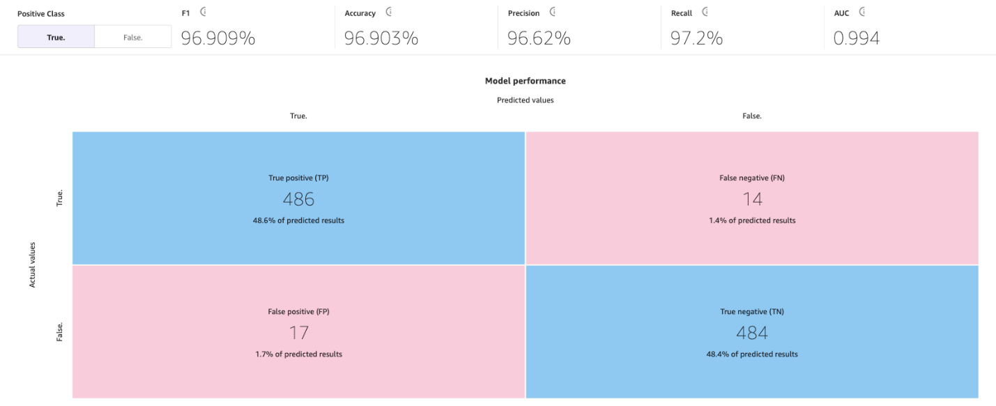
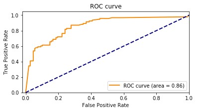
For our experiment, we use an example protein sequence from the CASP14 competition, which provides an independent mechanism for the assessment of methods of protein structure modeling. The target T1030 is derived from the PDB 6P00 protein, and has 237 amino acids in the primary sequence. We run the SageMaker pipeline to predict the protein structure of this input sequence with both OpenFold and AlphaFold algorithms.

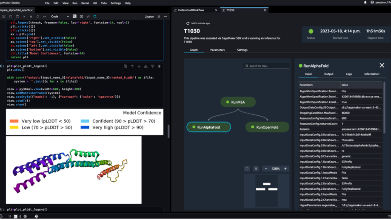
When the pipeline is complete, we download the predicted .pdb files from each folding job and visualize the structure in the notebook using py3Dmol, as in the notebook 04-compare_alphafold_openfold.ipynb.

The following screenshot shows the prediction from the AlphaFold prediction job.

The predicted structure is compared against its known base reference structure with PDB code 6poo archived in RCSB. We analyze the prediction performance against the base PDB code 6poo with three metrics: RMSD, RMSD with superposition, and template modeling score, as described in Comparing structures.

The folding algorithms are now compared against each other for multiple FASTA sequences: T1030, T1090, and T1076. New target sequences may not have the base pdb structure in reference databases and therefore it’s useful to compare the variability between folding algorithms.

The following screenshot shows the runs of ProteinFoldWorkflow for the three FASTA input sequences with SageMaker Pipeline:

We also log the metrics with SageMaker Experiments as new runs of the same experiment created by the pipeline:

from sagemaker.experiments.run import Run, load_run
metric_type='compare:'
experiment_name = 'proteinfoldworkflow'
with Run(experiment_name=experiment_name, run_name=input_name_1, sagemaker_session=sess) as run:
run.log_metric(name=metric_type + "rmsd_cur", value=rmsd_cur_one, step=1)
run.log_metric(name=metric_type + "rmds_fit", value=rmsd_fit_one, step=1)
run.log_metric(name=metric_type + "tm_score", value=tmscore_one, step=1)

We then analyze and visualize these runs on the Experiments page in SageMaker Studio.

The following chart depicts the RMSD value between AlphaFold and OpenFold for the three sequences: T1030, T1076, and T1090.

Conclusion

In this post, we described how you can use SageMaker Pipelines to set up and run protein folding workflows with two popular structure prediction algorithms: AlphaFold2 and OpenFold. We demonstrated a price performant solution architecture of multiple jobs that separates the compute requirements for MSA generation from structure prediction. We also highlighted how you can visualize, evaluate, and compare predicted 3D structures of proteins in SageMaker Studio.

To get started with protein folding workflows on SageMaker, refer to the sample code in the GitHub repo.

About the authors

Michael Hsieh is a Principal AI/ML Specialist Solutions Architect. He works with HCLS customers to advance their ML journey with AWS technologies and his expertise in medical imaging. As a Seattle transplant, he loves exploring the great mother nature the city has to offer, such as the hiking trails, scenery kayaking in the SLU, and the sunset at Shilshole Bay.

Shivam Patel is a Solutions Architect at AWS. He comes from a background in R&D and combines this with his business knowledge to solve complex problems faced by his customers. Shivam is most passionate about workloads in machine learning, robotics, IoT, and high-performance computing.

Hasan Poonawala is a Senior AI/ML Specialist Solutions Architect at AWS, Hasan helps customers design and deploy machine learning applications in production on AWS. He has over 12 years of work experience as a data scientist, machine learning practitioner, and software developer. In his spare time, Hasan loves to explore nature and spend time with friends and family.

Jasleen Grewal is a Senior Applied Scientist at Amazon Web Services, where she works with AWS customers to solve real world problems using machine learning, with special focus on precision medicine and genomics. She has a strong background in bioinformatics, oncology, and clinical genomics. She is passionate about using AI/ML and cloud services to improve patient care.

Read More

If you are a business analyst, understanding customer behavior is probably one of the most important things you care about. Understanding the reasons and mechanisms behind customer purchase decisions can facilitate revenue growth. However, the loss of customers (commonly referred to as customer churn) always poses a risk. Gaining insights into why customers leave can be just as crucial for sustaining profits and revenue.

Although machine learning (ML) can provide valuable insights, ML experts were needed to build customer churn prediction models until the introduction of Amazon SageMaker Canvas.

SageMaker Canvas is a low-code/no-code managed service that allows you to create ML models that can solve many business problems without writing a single line of code. It also enables you to evaluate the models using advanced metrics as if you were a data scientist.

In this post, we show how a business analyst can evaluate and understand a classification churn model created with SageMaker Canvas using the Advanced metrics tab. We explain the metrics and show techniques to deal with data to obtain better model performance.

Prerequisites

If you would like to implement all or some of the tasks described in this post, you need an AWS account with access to SageMaker Canvas. Refer to Predict customer churn with no-code machine learning using Amazon SageMaker Canvas to cover the basics around SageMaker Canvas, the churn model, and the dataset.

Introduction to model performance evaluation

As a general guideline, when you need to evaluate the performance of a model, you’re trying to measure how well the model will predict something when it sees new data. This prediction is called inference. You start by training the model using existing data, and then ask the model to predict the outcome on data that it has not already seen. How accurately the model predicts this outcome is what you look at to understand the model performance.

If the model hasn’t seen the new data, how would anybody know if the prediction is good or bad? Well, the idea is to actually use historical data where the results are already known and compare the these values to the model’s predicted values. This is enabled by setting aside a portion of the historical training data so it can be compared with what the model predicts for those values.

In the example of customer churn (which is a categorical classification problem), you start with a historical dataset that describes customers with many attributes (one in each record). One of the attributes, called Churn, can be True or False, describing if the customer left the service or not. To evaluate model accuracy, we split this dataset and train the model using one part (the training dataset), and ask the model to predict the outcome (classify the customer as Churn or not) with the other part (the test dataset). We then compare the model’s prediction to the ground truth contained in the test dataset.

Interpreting advanced metrics

In this section, we discuss the advanced metrics in SageMaker Canvas that can help you understand model performance.

Confusion matrix

SageMaker Canvas uses confusion matrices to help you visualize when a model generates predictions correctly. In a confusion matrix, your results are arranged to compare the predicted values against the actual historical (known) values. The following example explains how a confusion matrix works for a two-category prediction model that predicts positive and negative labels:

• True positive – The model correctly predicted positive when the true label was positive
• True negative – The model correctly predicted negative when the true label was negative
• False positive – The model incorrectly predicted positive when the true label was negative
• False negative – The model incorrectly predicted negative when the true label was positive

The following image is an example of a confusion matrix for two categories. In our churn model, the actual values come from the test dataset, and the predicted values come from asking our model.

Accuracy

Accuracy is the percentage of correct predictions out of all the rows or samples of the test set. It is the true samples that were predicted as True, plus the false samples that were correctly predicted as False, divided by the total number of samples in the dataset.

It’s one of the most important metrics to understand because it will tell you in what percentage the model correctly predicted, but it can be misleading in some cases. For example:

• Class imbalance – When the classes in your dataset are not evenly distributed (you have a disproportionate number of samples from one class and very little on others), accuracy can be misleading. In such cases, even a model that simply predicts the majority class for every instance can achieve a high accuracy.
• Cost-sensitive classification – In some applications, the cost of misclassification for different classes can be different. For example, if we were predicting if a drug can aggravate a condition, a false negative (for example, predicting the drug might not aggravate when it actually does) can be more costly than a false positive (for example, predicting the drug might aggravate when it actually does not).

Precision, recall, and F1 score

Precision is the fraction of true positives (TP) out of all the predicted positives (TP + FP). It measures the proportion of positive predictions that are actually correct.

Recall is the fraction of true positives (TP) out of all the actual positives (TP + FN). It measures the proportion of positive instances that were correctly predicted as positive by the model.

The F1 score combines precision and recall to provide a single score that balances the trade-off between them. It is defined as the harmonic mean of precision and recall:

F1 score = 2 * (precision * recall) / (precision + recall)

The F1 score ranges from 0–1, with a higher score indicating better performance. A perfect F1 score of 1 indicates that the model has achieved both perfect precision and perfect recall, and a score of 0 indicates that the model’s predictions are completely wrong.

The F1 score provides a balanced evaluation of the model’s performance. It considers precision and recall, providing a more informative evaluation metric that reflects the model’s ability to correctly classify positive instances and avoid false positives and false negatives.

For example, in medical diagnosis, fraud detection, and sentiment analysis, F1 is especially relevant. In medical diagnosis, accurately identifying the presence of a specific disease or condition is crucial, and false negatives or false positives can have significant consequences. The F1 score takes into account both precision (the ability to correctly identify positive cases) and recall (the ability to find all positive cases), providing a balanced evaluation of the model’s performance in detecting the disease. Similarly, in fraud detection, where the number of actual fraud cases is relatively low compared to non-fraudulent cases (imbalanced classes), accuracy alone may be misleading due to a high number of true negatives. The F1 score provides a comprehensive measure of the model’s ability to detect both fraudulent and non-fraudulent cases, considering both precision and recall. And in sentiment analysis, if the dataset is imbalanced, accuracy may not accurately reflect the model’s performance in classifying instances of the positive sentiment class.

AUC (area under the curve)

The AUC metric evaluates the ability of a binary classification model to distinguish between positive and negative classes at all classification thresholds. A threshold is a value used by the model to make a decision between the two possible classes, converting the probability of a sample being part of a class into a binary decision. To calculate the AUC, the true positive rate (TPR) and false positive rate (FPR) are plotted across various threshold settings. The TPR measures the proportion of true positives out of all actual positives, while the FPR measures the proportion of false positives out of all actual negatives. The resulting curve, called the receiver operating characteristic (ROC) curve, provides a visual representation of the TPR and FPR at different threshold settings. The AUC value, which ranges from 0–1, represents the area under the ROC curve. Higher AUC values indicate better performance, with a perfect classifier achieving an AUC of 1.

The following plot shows the ROC curve, with TPR as the Y axis and FPR as the X axis. The closer the curve gets to the top left corner of the plot, the better the model does at classifying the data into categories.

To clarify, let’s go over an example. Let’s think about a fraud detection model. Usually, these models are trained from unbalanced datasets. This is due to the fact that, usually, almost all the transactions in the dataset are non-fraudulent with only a few labeled as frauds. In this case, the accuracy alone may not adequately capture the performance of the model because it is probably heavily influenced by the abundance of non-fraudulent cases, leading to misleadingly high accuracy scores.

In this case, the AUC would be a better metric to assess model performance because it provides a comprehensive assessment of a model’s ability to distinguish between fraudulent and non-fraudulent transactions. It offers a more nuanced evaluation, taking into account the trade-off between true positive rate and false positive rate at various classification thresholds.

Just like the F1 score, it is particularly useful when the dataset is imbalanced. It measures the trade-off between TPR and FPR and shows how well the model can differentiate between the two classes regardless of their distribution. This means that even if one class is significantly smaller than the other, the ROC curve assesses the model’s performance in a balanced manner by considering both classes equally.

Additional key topics

Advanced metrics are not the only important tools available to you for evaluating and improving ML model performance. Data preparation, feature engineering, and feature impact analysis are techniques that are essential to model building. These activities play a crucial role in extracting meaningful insights from raw data and improving model performance, leading to more robust and insightful results.

Data preparation and feature engineering

Feature engineering is the process of selecting, transforming, and creating new variables (features) from raw data, and plays a key role in improving the performance of an ML model. Selecting the most relevant variables or features from the available data involves removing irrelevant or redundant features that do not contribute to the model’s predictive power. Transforming data features into a suitable format includes scaling, normalization, and handling missing values. And finally, creating new features from the existing data is done through mathematical transformations, combining or interacting different features, or creating new features from domain-specific knowledge.

Feature importance analysis

SageMaker Canvas generates a feature importance analysis that explains the impact that each column in your dataset has on the model. When you generate predictions, you can see the column impact that identifies which columns have the most impact on each prediction. This will give you insights on which features deserve to be part of your final model and which ones should be discarded. Column impact is a percentage score that indicates how much weight a column has in making predictions in relation to the other columns. For a column impact of 25%, Canvas weighs the prediction as 25% for the column and 75% for the other columns.

Approaches to improve model accuracy

Although there are multiple methods to improve model accuracy, data scientists and ML practitioners usually follow one of the two approaches discussed in this section, using the tools and metrics described earlier.

Model-centric approach

In this approach, the data always remains the same and is used to iteratively improve the model to meet desired results. Tools used with this approach include:

• Trying multiple relevant ML algorithms
• Algorithm and hyperparameter tuning and optimization
• Different model ensemble methods
• Using pre-trained models (SageMaker provides various built-in or pre-trained models to help ML practitioners)
• AutoML, which is what SageMaker Canvas does behind the scenes (using Amazon SageMaker Autopilot), which encompasses all of the above

Data-centric approach

In this approach, the focus is on data preparation, improving data quality, and iteratively modifying the data to improve performance:

• Exploring statistics of the dataset used to train the model, also known as exploratory data analysis (EDA)
• Improving data quality (data cleaning, missing values imputation, outlier detection and management)
• Feature selection
• Feature engineering
• Data augmentation

Improving model performance with Canvas

We begin with the data-centric approach. We use the model preview functionality to perform an initial EDA. This provides us a baseline that we can use to perform data augmentation, generating a new baseline, and finally getting the best model with a model-centric approach using the standard build functionality.

We use the synthetic dataset from a telecommunications mobile phone carrier. This sample dataset contains 5,000 records, where each record uses 21 attributes to describe the customer profile. Refer to Predict customer churn with no-code machine learning using Amazon SageMaker Canvas for a full description.

Model preview in a data-centric approach

As a first step, we open the dataset, select the column to predict as Churn?, and generate a preview model by choosing Preview model.

The Preview model pane will show the progress until the preview model is ready.

When the model is ready, SageMaker Canvas generates a feature importance analysis.

Finally, when it’s complete, the pane will show a list of columns with its impact on the model. These are useful to understand how relevant the features are on our predictions. Column impact is a percentage score that indicates how much weight a column has in making predictions in relation to the other columns. In the following example, for the Night Calls column, SageMaker Canvas weights the prediction as 4.04% for the column and 95.9% for the other columns. The higher the value, the higher the impact.

As we can see, the preview model has a 95.6% accuracy. Let’s try to improve the model performance using a data-centric approach. We perform data preparation and use feature engineering techniques to improve performance.

As shown in the following screenshot, we can observe that the Phone and State columns have much less impact on our prediction. Therefore, we will use this information as input for our next phase, data preparation.

SageMaker Canvas provides ML data transforms with which you can clean, transform, and prepare your data for model building. You can use these transforms on your datasets without any code, and they will be added to the model recipe, which is a record of the data preparation performed on your data before building the model.

Note that any data transforms you use only modify the input data when building a model and do not modify your dataset or original data source.

The following transforms are available in SageMaker Canvas for you to prepare your data for building:

• Datetime extraction
• Drop columns
• Filter rows
• Functions and operators
• Manage rows
• Rename columns
• Remove rows
• Replace values
• Resample time series data

Let’s start by dropping the columns we have found that have little impact on our prediction.

For example, in this dataset, the phone number is just the equivalent of an account number—it’s useless or even detrimental in predicting other accounts’ likelihood of churn. Likewise, the customer’s state doesn’t impact our model much. Let’s remove the Phone and State columns by unselecting those features under Column name.

Now, let’s perform some additional data transformation and feature engineering.

For example, we noticed in our previous analysis that the charged amount to customers has a direct impact on churn. Let’s therefore create a new column that computes the total charges to our customers by combining Charge, Mins, and Calls for Day, Eve, Night, and Intl. To do so, we use the custom formulas in SageMaker Canvas.

Let’s start by choosing Functions, then we add to the formula textbox the following text:

(Day Calls*Day Charge*Day Mins)+(Eve Calls*Eve Charge*Eve Mins)+(Night Calls*Night Charge*Night Mins)+(Intl Calls*Intl Charge*Intl Mins)

Give the new column a name (for example, Total Charges), and choose Add after the preview has been generated. The model recipe should now look as shown in the following screenshot.

When this data preparation is complete, we train a new preview model to see if the model improved. Choose Preview model again, and the lower right pane will show the progress.

When training is finished, it will proceed to recompute the predicted accuracy, and will also create a new column impact analysis.

And finally, when the whole process is complete, we can see the same pane we saw earlier but with the new preview model accuracy. You can notice model accuracy increased by 0.4% (from 95.6% to 96%).

The numbers in the preceding images may differ from yours because ML introduces some stochasticity in the process of training models, which can lead to different results in different builds.

Model-centric approach to create the model

Canvas offers two options to build your models:

• Standard build – Builds the best model from an optimized process where speed is exchanged for better accuracy. It uses Auto-ML, which automates various tasks of ML, including model selection, trying various algorithms relevant to your ML use case, hyperparameter tuning, and creating model explainability reports.
• Quick build – Builds a simple model in a fraction of the time compared to a standard build, but accuracy is exchanged for speed. Quick model is useful when iterating to more quickly understand the impact of data changes to your model accuracy.

Let’s continue using a standard build approach.

Standard build

As we saw before, the standard build builds the best model from an optimized process to maximize accuracy.

The build process for our churn model takes around 45 minutes. During this time, Canvas tests hundreds of candidate pipelines, selecting the best model. In the following screenshot, we can see the expected build time and progress.

With the standard build process, our ML model has improved our model accuracy to 96.903%, which is a significant improvement.

Explore advanced metrics

Let’s explore the model using the Advanced metrics tab. On the Scoring tab, choose Advanced metrics.

This page will show the following confusion matrix jointly with the advanced metrics: F1 score, accuracy, precision, recall, F1 score, and AUC.

Generate predictions

Now that the metrics look good, we can perform an interactive prediction on the Predict tab, either in a batch or single (real-time) prediction.

We have two options:

• Use this model to run to run batch or single predictions
• Send the model to Amazon Sagemaker Studio to share with data scientists

Clean up

To avoid incurring future session charges, log out of SageMaker Canvas.

Conclusion

SageMaker Canvas provides powerful tools that enable you to build and assess the accuracy of models, enhancing their performance without the need for coding or specialized data science and ML expertise. As we have seen in the example through the creation of a customer churn model, by combining these tools with both a data-centric and a model-centric approach using advanced metrics, business analysts can create and evaluate prediction models. With a visual interface, you’re also empowered to generate accurate ML predictions on your own. We encourage you to go through the references and see how many of these concepts might apply in other types of ML problems.

References

• Predict customer churn with no-code machine learning using Amazon SageMaker Canvas
• Build, Share, Deploy: how business analysts and data scientists achieve faster time-to-market using no-code ML and Amazon SageMaker Canvas
• Customizing and reusing models generated by Amazon SageMaker Autopilot
• Amazon SageMaker Canvas Immersion Day Workshop
• Manage AutoML workflows with AWS Step Functions and AutoGluon on Amazon SageMaker

About the Authors

Marcos is an AWS Sr. Machine Learning Solutions Architect based in Florida, US. In that role, he is responsible for guiding and assisting US startup organizations in their strategy towards the cloud, providing guidance on how to address high-risk issues and optimize their machine learning workloads. He has more than 25 years of experience with technology, including cloud solution development, machine learning, software development, and data center infrastructure.

Indrajit is an AWS Enterprise Sr. Solutions Architect. In his role, he helps customers achieve their business outcomes through cloud adoption. He designs modern application architectures based on microservices, serverless, APIs, and event-driven patterns. He works with customers to realize their data analytics and machine learning goals through adoption of DataOps and MLOps practices and solutions. Indrajit speaks regularly at AWS public events like summits and ASEAN workshops, has published several AWS blog posts, and developed customer-facing technical workshops focused on data and machine learning on AWS.

Read More