Monthly Archives: January 2023

Amazon SageMaker provides a suite of built-in algorithms, pre-trained models, and pre-built solution templates to help data scientists and machine learning (ML) practitioners get started on training and deploying ML models quickly. You can use these algorithms and models for both supervised and unsupervised learning. They can process various types of input data, including tabular, image, and text.

Starting today, the SageMaker LightGBM algorithm offers distributed training using the Dask framework for both tabular classification and regression tasks. They’re available through the SageMaker Python SDK. The supported data format can be either CSV or Parquet. Extensive benchmarking experiments on four publicly available datasets with various settings are conducted to validate its performance.

Customers are increasingly interested in training models on large datasets with SageMaker LightGBM, which can take a day or even longer. In these cases, you might be able to speed up the process by distributing training over multiple machines or processes in a cluster. This post discusses how SageMaker LightGBM helps you set up and launch distributed training, without the expense and difficulty of directly managing your training clusters.

Problem statement

Machine learning has become an essential tool for extracting insights from large amounts of data. From image and speech recognition to natural language processing and predictive analytics, ML models have been applied to a wide range of problems. As datasets continue to grow in size and complexity, traditional training methods can become increasingly time-consuming and resource-intensive. This is where distributed training comes into play.

Distributed training is a technique that allows for the parallel processing of large amounts of data across multiple machines or devices. By splitting the data and training multiple models in parallel, distributed training can significantly reduce training time and improve the performance of models on big data. In recent years, distributed training has been a popular mechanism in training deep neural networks for use cases such as large language models (LLMs), image generation and classification, and text generation tasks using frameworks like PyTorch, TensorFlow, and MXNet. In this post, we discuss how distributed training can be applied to tabular data (a common type of data found in many industries such as finance, healthcare, and retail) using Dask and the LightGBM algorithm for tasks such as regression and classification.

Dask is an open-source parallel computing library that allows for distributed parallel processing of large datasets in Python. It’s designed to work with the existing Python and data science ecosystem such as NumPy and Pandas. When it comes to distributed training, Dask can be used to parallelize the data loading, preprocessing, and model training tasks, and it integrates well with popular ML algorithms like LightGBM. LightGBM is a gradient boosting framework that uses tree-based learning algorithms, which is designed to be efficient and scalable for training large models on big data. Combining these two powerful libraries, LightGBM v3.2.0 is now integrated with Dask to allow distributed learning across multiple machines to produce a single model.

How distributed training works

Distributed training for tree-based algorithms is a technique that is used when the dataset is too large to be processed on a single instance or when the computational resources of a single instance are not sufficient to train the tree-based model in a reasonable amount of time. It allows a model to be trained across multiple instances or machines, rather than on a single machine. This is done by dividing the dataset into smaller subsets, called chunks, and distributing them among the available instances. Each instance then trains a model on its assigned chunk of data, and the results are later combined using aggregation algorithms to form a single model.

In tree-based models like LightGBM, the main computational cost is in the building of the tree structure. This is typically done by sorting and selecting subsets of the data.

Now, let’s explore how LightGBM does the parallel training. LightGBM can use three types of parallelism:

• Data parallelism – This is the most basic form of data parallelism. The data is divided horizontally into smaller subsets and distributed among multiple instances. Each instance constructs its local histogram, and all histograms are merged, then a split is performed using a reduce scatter algorithm. A histogram in local instances is constructed by dividing the subset of the local data into discrete bins, and counting the number of data points in each bin. This histogram-based algorithm helps speed up the training and reduces memory usage.
• Feature parallelism – In feature parallelism, each machine is responsible for training a subset of the features of the model, rather than a subset of the data. This can be useful when working with datasets that have a large number of features, because it allows for more efficient use of resources. It works by finding the best local split point in each instance, then communicates the best split with the other instances. LightGBM implementation maintains all features of the data in every machine to reduce the cost of communicating the best splits.
• Voting parallelism – In voting parallelism, the data is divided into smaller subsets and distributed among multiple machines. Each machine trains a model on its assigned subset of data, and the results are later combined to form a single, larger model. However, instead of using the gradients from all the machines to update the model parameters, a voting mechanism is used to decide which gradients to use. This can be useful when working with datasets that have a lot of noise or outliers, because it can help reduce the impact of these on the final model. At the time of writing this post, LightGBM integration with Dask only supports data and voting parallelism types.

SageMaker will automatically set up and manage a Dask cluster when using multiple instances with the LightGBM built-in container.

Solution overview

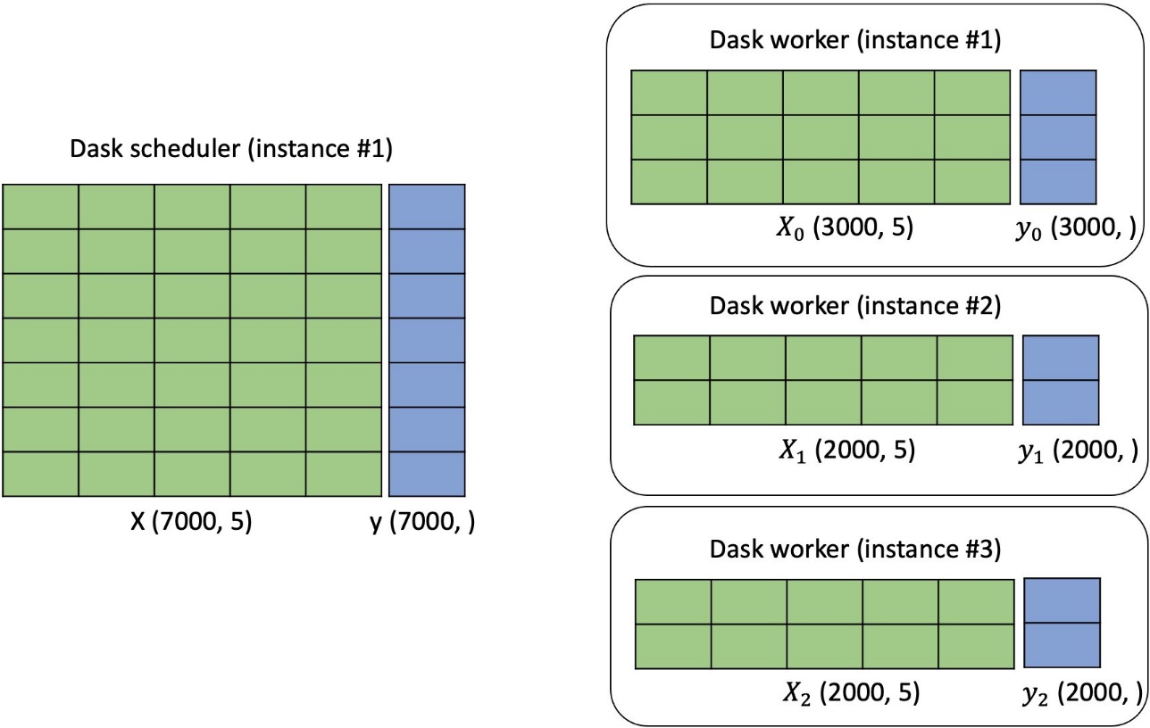
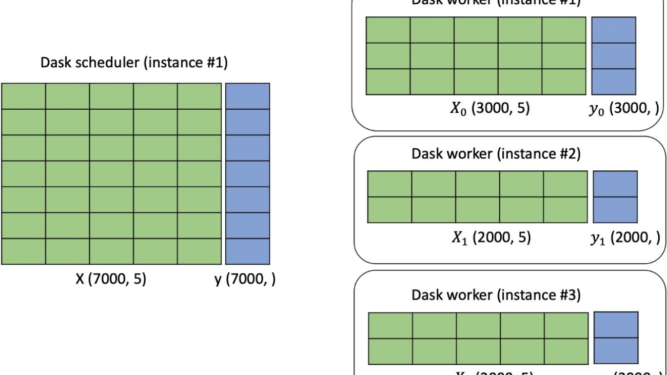
When a training job using LightGBM is started with multiple instances, we first create a Dask cluster. One instance acts as the Dask scheduler, and the remaining instances have Dask workers, where each worker has multiple threads. Each worker in the cluster has part of the data to perform the distributed computations, as illustrated in the following figure.

Enable distributed training

The requirements for the input data are as follows:

• The supported input data format for training can be either CSV or Parquet. You are allowed to put more than one data file under both train and validation channels. If multiple files are identified, the algorithm will concatenate all of them as the training or validation data. The name of the data file can be any string as long as it ends with .csv or .parquet.
• For each data file, the algorithm requires that the target variable is in the first column and that it should not have a header record. This follows the convention of the SageMaker XGBoost algorithm.
• If your predictors include categorical features, you can provide a JSON file named cat_index.json in the same location as your training data. This file should contain a Python dictionary, where the key can be any string and the value is a list of unique integers. Each integer in the value list should indicate the column index of the corresponding categorical features in your data file. The index starts with value 1, because value 0 corresponds to the target variable. The cat_index.json file should be put under the training data directory, as shown in the following example.
• The instance type supported by distributed training is CPU.

Let’s use data in CSV format as an example. The train and validation data can be structured as follows:

-- training_dataset_s3_path
    -- data_1.csv
    -- data_2.csv
    -- data_3.csv
    -- cat_idx.json
    
-- validation_dataset_s3_path
    -- data_1.csv

You can specify the input type to be either text/csv or application/x-parquet:

from sagemaker.inputs import TrainingInput

content_type = "text/csv" # or "application/x-parquet"

train_input = TrainingInput(
    training_dataset_s3_path, content_type=content_type
)

validation_input = TrainingInput(
    validation_dataset_s3_path, content_type=content_type
)

Before distributed training, you can retrieve the default hyperparameters of LightGBM and override them with custom values:

from sagemaker import hyperparameters

# Retrieve the default hyper-parameters for LightGBM
hyperparameters = hyperparameters.retrieve_default(
    model_id=train_model_id, model_version=train_model_version
)

# [Optional] Override default hyperparameters with custom values
hyperparameters[
    "num_boost_round"
] = "500" 

hyperparameters["tree_learner"] = "voting" ### specify either 'data' or 'voting' parallelism for distributed training. Unfortnately, for dask lightgbm, the 'feature' is not supported. See github issue: https://github.com/microsoft/LightGBM/issues/3834

To enable distributed training, you can simply specify the argument instance_count in the class sagemaker.estimator.Estimator to be more than 1. The rest of work is taken care of under the hood. See the following example code:

from sagemaker.estimator import Estimator
from sagemaker.utils import name_from_base

training_job_name = name_from_base("sagemaker-built-in-distributed-lgb")

# Create SageMaker Estimator instance
tabular_estimator = Estimator(
    role=aws_role,
    image_uri=train_image_uri,
    source_dir=train_source_uri,
    model_uri=train_model_uri,
    entry_point="transfer_learning.py",
    instance_count=4, ### select the instance count you would like to use for distributed training
    volume_size=30, ### volume_size (int or PipelineVariable): Size in GB of the storage volume to use for storing input and output data during training (default: 30).
    instance_type=training_instance_type,
    max_run=360000,
    hyperparameters=hyperparameters,
    output_path=s3_output_location,
)

# Launch a SageMaker Training job by passing s3 path of the training data
tabular_estimator.fit(
    {
        "train": train_input,
        "validation": validation_input,
    }, logs=True, job_name=training_job_name
)

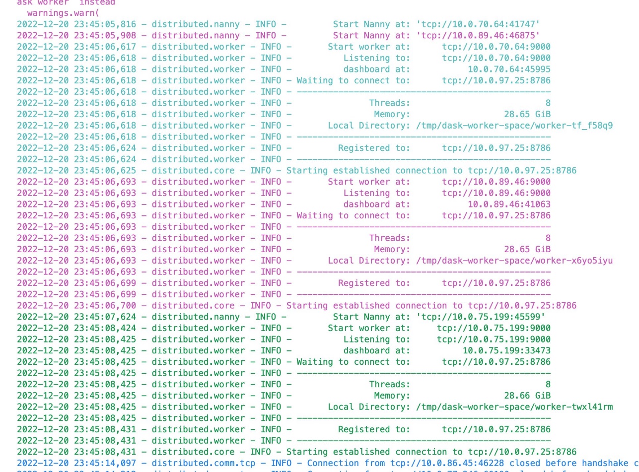
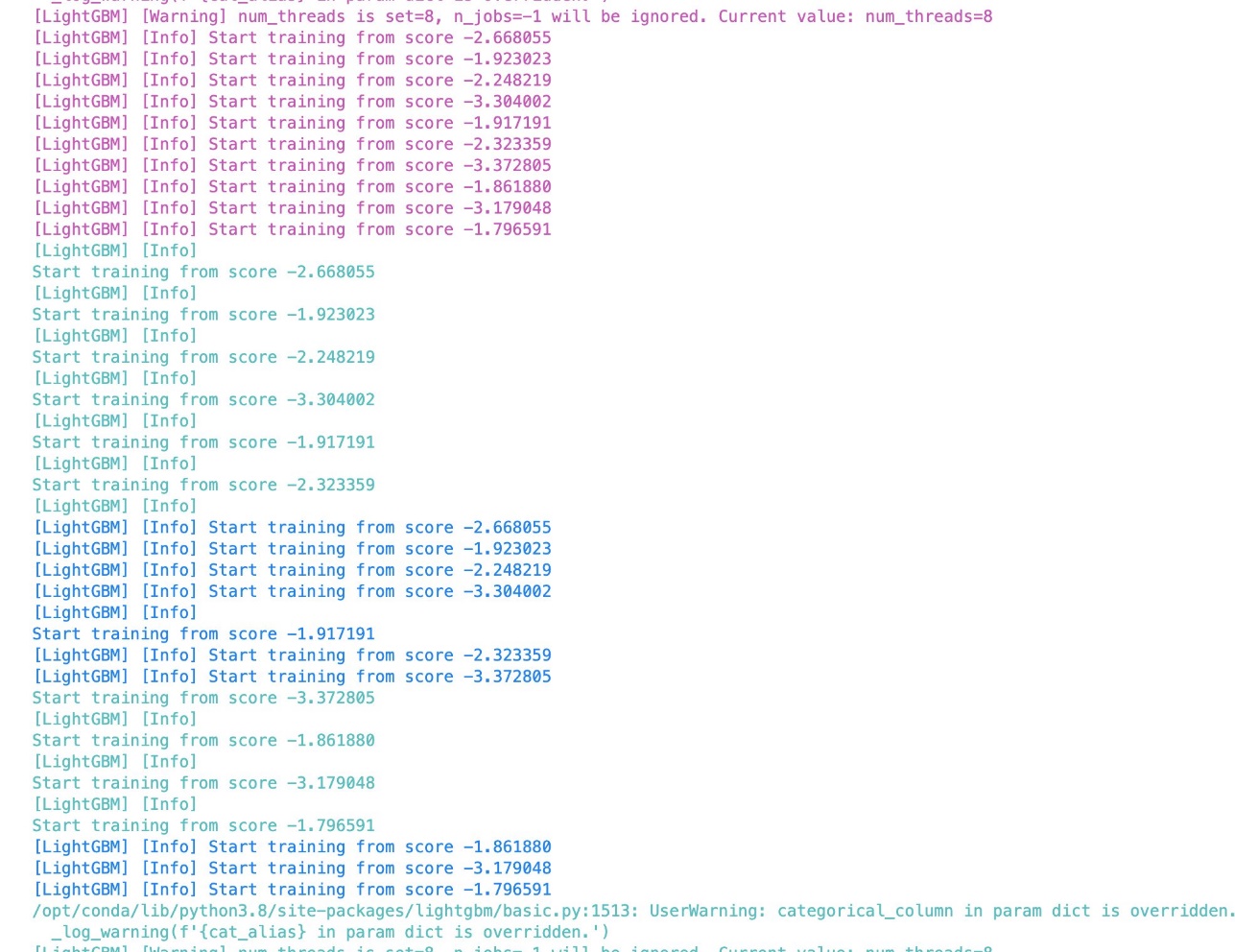
The following screenshots show a successful training job log from the notebook. The logs from different Amazon Elastic Compute Cloud (Amazon EC2) machines are marked by different colors.

The distributed training is also compatible with SageMaker automatic model tuning. For details, see the example notebook.

Benchmarking

We conducted benchmarking experiments to validate the performance of distributed training in SageMaker LightGBM on four different publicly available datasets for regression, binary, and multi-class classification tasks. The experiment details are as follows:

• Each dataset is split into training, validation, and test data following the 80/20/10 split rule. For each dataset and instance type and count, we train LightGBM on the training data; record metrics such as billable time (per instance), total runtime, average training loss at the end of the last built tree over all instances, and validation loss at the end of the last built tree; and evaluate its performance on the hold-out test data.
• For each trial, we use the exact same set of hyperparameter values, with the number of trees being 500 except for the lending dataset. For the lending dataset, we use 100 as the number of trees because it’s sufficient to get optimal results on the hold-out test data.
• Each number presented in the table is averaged over three trials.
• Because each model is trained with one fixed set of hyperparameter values, the evaluation metric numbers on the hold-out test data can be further improved with hyperparameter optimization.

Billable time refers to the absolute wall-clock time. The total runtime is the elastic time running the distributed training, which includes the billable time and time to spin up instances and install dependencies. For the validation loss at the end of the last built tree, we didn’t do the average over all the instances as the training loss because all of the validation data is assigned to a single instance and therefore only that instance has the validation loss metric. Out of Memory (OOM) means the dataset hit the out of memory error during training. The loss function and evaluation metrics used are binary and multi-class logloss, L2, accuracy, F1, ROC AUC, F1 macro, F1 micro, R2, MAE, and MSE.

The expectation is that as the instance count increases, the billable time (per instance) and total runtime decreases, while the average training loss and validation loss at the end of the last built tree and evaluation scores on the hold-out test data remain the same.

We conducted three experiments:

• Benchmark on three publicly available datasets using CSV as the input data format
• Benchmark on a different dataset using Parquet as the input data format
• Compare the model performance on different instance types given a certain instance count

The datasets we used are lending club loan data, ad-tracking fraud detection data, code data, and NYC taxi data. The data statistics are presented as follows.

The following table contains the benchmarking results for the first three datasets using CSV as the data input format. For demonstration purposes, we removed the categorical features for the lending club loan data. The data statistics are shown in the table. The experiment results matched our expectations.

The following table contains the benchmarking results using NYC taxi data with Parquet as the input data format. For the NYC taxi data, we use the yellow trip taxi records from 2009–2022. We follow the example notebook to conduct feature processing. The processed data takes 8.5 G of disk memory when saved as CSV format, and only 0.55 G when saved as Parquet format.

A similar pattern shown in the preceding table is observed. As the instance count increases, the billable time (per instance) and total runtime decreases, while the average training loss and validation loss at the end of the last built tree and evaluation scores on the hold-out test data remain the same.

We also conduct benchmarking experiments and compare the performance under different instance types using the code dataset. For a certain instance count, as the instance type becomes larger, the billable time and total runtime decrease.

Conclusion

With the power of Dask’s distributed computing framework and LightGBM’s efficient gradient boosting algorithm, data scientists and developers can train models on large datasets faster and more efficiently than using traditional single-node methods. The SageMaker LightGBM algorithm makes the process of setting up distributed training using the Dask framework for both tabular classification and regression tasks much easier. The algorithm is now available through the SageMaker Python SDK. The supported data format can be either CSV or Parquet. Extensive benchmarking experiments were conducted on four publicly available datasets with various settings to validate its performance.

You can bring your own dataset and try these new algorithms on SageMaker, and check out the example notebook to use the built-in algorithms available on GitHub.

About the authors

Dr. Xin Huang is an Applied Scientist for Amazon SageMaker JumpStart and Amazon SageMaker built-in algorithms. He focuses on developing scalable machine learning algorithms. His research interests are in the area of natural language processing, explainable deep learning on tabular data, and robust analysis of non-parametric space-time clustering. He has published many papers in ACL, ICDM, KDD conferences, and Royal Statistical Society: Series A journal.

Will Badr is a Principal AI/ML Specialist SA who works as part of the global Amazon Machine Learning team. Will is passionate about using technology in innovative ways to positively impact the community. In his spare time, he likes to go diving, play soccer and explore the Pacific Islands.

Dr. Li Zhang is a Principal Product Manager-Technical for Amazon SageMaker JumpStart and Amazon SageMaker built-in algorithms, a service that helps data scientists and machine learning practitioners get started with training and deploying their models, and uses reinforcement learning with Amazon SageMaker. His past work as a principal research staff member and master inventor at IBM Research has won the test of time paper award at IEEE INFOCOM.

Read More

Amazon Forecast is a fully managed service that uses machine learning (ML) to generate highly accurate forecasts, without requiring any prior ML experience. Forecast is applicable in a wide variety of use cases, including estimating supply and demand for inventory management, travel demand forecasting, workforce planning, and computing cloud infrastructure usage.

You can use Forecast to seamlessly conduct what-if analyses up to 80% faster to analyze and quantify the potential impact of business levers on your demand forecasts. A what-if analysis helps you investigate and explain how different scenarios might affect the baseline forecast created by Forecast. With Forecast, there are no servers to provision or ML models to build manually. Additionally, you only pay for what you use, and there is no minimum fee or upfront commitment. To use Forecast, you only need to provide historical data for what you want to forecast, and, optionally, any additional data that you believe may impact your forecasts.

Water utility providers have several forecasting use cases, but primary among them is predicting water consumption in an area or building to meet the demand. Also, it’s important for utility providers to forecast the increased consumption demand because of more apartments added in a building or more houses in the area. Predicting water consumption accurately is critical to avoid any service interruptions to the customer.

This post explores using Forecast to address this use case by using historical time series data.

Solution overview

Water is a natural resource and very critical to industry, agriculture, households, and our lives. Accurate water consumption forecasting is critical to make sure that an agency can run day-to-day operations efficiently. Water consumption forecasting is particularly challenging because demand is dynamic, and seasonal weather changes can have an impact. Predicting water consumption accurately is important so customers don’t face any service interruptions and in order to provide a stable service while maintaining low prices. Improved forecasting enables you to plan ahead to structure more cost-effective future contracts. The following are the two most common use cases:

• Better demand management – As a utility provider agency, you need to find a balance between water demand and supply. The agency collects information like number of people living in an apartment and number of apartments in a building before providing service. As a utility agency, you must balance aggregate supply and demand. You need to store sufficient water in order to meet the demand. Moreover, demand forecasting has become more challenging for the following reasons:
  • The demand isn’t stable at all times and varies throughout the day. For example, water consumption at midnight is much less compared to in the morning.
  • Weather can also have an impact on the overall consumption. For example, water consumption is higher in the summer than the winter in the northern hemisphere, and the other way around in the southern hemisphere.
  • There is not enough rainfall or water storage mechanisms (lakes, reservoirs), or water filtering is insufficient. During the summer, demand can’t always keep up with supply. The water agencies have to forecast carefully to acquire other sources, which may be more expensive. Therefore, it’s critical for utility agencies to find alternative water sources like harvesting rainwater, capturing condensation from air handling units, or reclaiming wastewater.
• Conducting a what-if analysis for increased demand – Demand for water is rising due to multiple reasons. This includes a combination of population growth, economic development, and changing consumption patterns. Let’s imagine a scenario where an existing apartment building builds an extension and the number of households and people increase by a certain percentage. Now you need to do an analysis to forecast the supply for increased demand. This also helps you make a cost-effective contract for increased demand.

Forecasting can be challenging because you first need accurate models to forecast demand and then a quick and simple way to reproduce the forecast across a range of scenarios.

This post focuses on a solution to perform water consumption forecasting and a what-if analysis. This post doesn’t consider weather data for model training. However, you can add weather data, given its correlation to water consumption.

Prerequisites

Before getting started, we set up our resources. For this post, we use the us-east-1 Region.

1. Create an Amazon Simple Storage Service (Amazon S3) bucket for storing the historical time series data. For instructions, refer to Create your first S3 bucket.
2. Download data files from the GitHub repo and upload to the newly created S3 bucket.
3. Create a new AWS Identity and Access Management (IAM) role. For instructions, see Set Up Permissions for Amazon Forecast. Be sure to provide the name of your S3 bucket.

Create a dataset group and datasets

This post demonstrates two use cases related to water demand forecast: forecasting the water demand based on past water consumption, and conducting a what-if analysis for increased demand.

Forecast can accept three types of datasets: target time series (TTS), related time series (RTS), and item metadata (IM). Target time series data defines the historical demand for the resources you’re predicting. The target time series dataset is mandatory. A related time series dataset includes time-series data that isn’t included in a target time series dataset and might improve the accuracy of your predictor.

In our example, the target time series dataset contains item_id and timestamp dimensions, and the complementary related time series dataset includes no_of_consumer. An important note with this dataset: the TTS ends on 2023-01-01, and the RTS ends on 2023-01-15. When performing what-if scenarios, it’s important to manipulate RTS variables beyond your known time horizon in TTS.

To conduct a what-if analysis, we need to import two CSV files representing the target time series data and the related time series data. Our example target time series file contains the item_id, timestamp, and demand, and our related time series file contains the product item_id, timestamp, and no_of consumer.

To import your data, complete the following steps:

1. On the Forecast console, choose View dataset groups.
   
   
2. Choose Create dataset group.
   
   
3. For Dataset group name, enter a name (for this post, water_consumption_datasetgroup).
4. For Forecasting domain, choose a forecasting domain (for this post, Custom).
5. Choose Next.
   
6. On the Create target time series dataset page, provide the dataset name, frequency of your data, and data schema.
   
7. On the Dataset import details page, enter a dataset import name.
8. For Import file type, select CSV and enter the data location.
9. Choose the IAM role you created earlier as a prerequisite.
10. Choose Start.
    

You’re redirected to the dashboard that you can use to track progress.

11. To import the related time series file, on the dashboard, choose Import.
    
12. On the Create related time series dataset page, provide the dataset name and data schema.
    
13. On the Dataset import details page, enter a dataset import name.
14. For Import file type, select CSV and enter the data location.
15. Choose the IAM role you created earlier.
16. Choose Start.
    

Train a predictor

Next, we train a predictor.

1. On the dashboard, choose Start under Train a predictor.
   
2. On the Train predictor page, enter a name for your predictor.
3. Specify how long in the future you want to forecast and at what frequency.
4. Specify the number of quantiles you want to forecast for.

Forecast uses AutoPredictor to create predictors. For more information, refer to Training Predictors.

5. Choose Create.

Create a forecast

After our predictor is trained (this can take approximately 3.5 hours), we create a forecast. You will know that your predictor is trained when you see the View predictors button on your dashboard.

1. Choose Start under Generate forecasts on the dashboard.
   
2. On the Create a forecast page, enter a forecast name.
3. For Predictor, choose the predictor that you created.
4. Optionally, specify the forecast quantiles.
5. Specify the items to generate a forecast for.
6. Choose Start.
   

Query your forecast

You can query a forecast using the Query forecast option. By default, the complete range of the forecast is returned. You can request a specific date range within the complete forecast. When you query a forecast, you must specify filtering criteria. A filter is a key-value pair. The key is one of the schema attribute names (including forecast dimensions) from one of the datasets used to create the forecast. The value is a valid value for the specified key. You can specify multiple key-value pairs. The returned forecast will only contain items that satisfy all the criteria.

1. Choose Query forecast on the dashboard.
   
2. Provide the filter criteria for start date and end date.
3. Specify your forecast key and value.
4. Choose Get Forecast.
   

The following screenshot shows the forecast energy consumption for the same apartment (item ID A_10001) using the forecast model.

Create a what-if analysis

At this point, we have created our baseline forecast can now conduct a what-if analysis. Let’s imagine a scenario where an existing apartment building adds an extension, and the number of households and people increases by 20%. Now you need to do an analysis to forecast increased supply based on increased demand.

There are three stages to conducting a what-if analysis: setting up the analysis, creating the what-if forecast by defining what is changed in the scenario, and comparing the results.

1. To set up your analysis, choose Explore what-if analysis on the dashboard.
   
2. Choose Create.
   
3. Enter a unique name and choose the baseline forecast.
4. Choose the items in your dataset you want to conduct a what-if analysis for. You have two options:
   • Select all items is the default, which we choose in this post.
   • If you want to pick specific items, choose Select items with a file and import a CSV file containing the unique identifier for the corresponding item and any associated dimensions.
5. Choose Create what-if analysis.
   

Create a what-if forecast

Next, we create a what-if forecast to define the scenario we want to analyze.

1. In the What-if forecast section, choose Create.
   
2. Enter a name of your scenario.
3. You can define your scenario through two options:
   • Use transformation functions – Use the transformation builder to transform the related time series data you imported. For this walkthrough, we evaluate how the demand for an item in our dataset changes when the number of consumers increases by 20% when compared to the price in the baseline forecast.
   • Define the what-if forecast with a replacement dataset – Replace the related time series dataset you imported.

For our example, we create a scenario where we increase no_of_consumer by 20% applicable to item ID A_10001, and no_of_consumer is a feature in the dataset. You need this analysis to forecast and meet the water supply for increased demand. This analysis also helps you make a cost-effective contract based on the water demand forecast.

4. For What-if forecast definition method, select Use transformation functions.
5. Choose Multiply as our operator, no_of_consumer as our time series, and enter 1.2.
6. Choose Add condition.
7. Choose Equals as the operation and enter A_10001 for item_id.
8. Choose Create.
   

Compare the forecasts

We can now compare the what-if forecasts for both our scenarios, comparing a 20% increase in consumers with the baseline demand.

1. On the analysis insights page, navigate to the Compare what-if forecasts section.
2. For item_id, enter the item to analyze (in our scenario, enter A_10001).
3. For What-if forecasts, choose water_demand_whatif_analyis.
4. Choose Compare what-if.
   
5. You can choose the baseline forecast for the analysis.

The following graph shows the resulting demand for our scenario. The red line shows the forecast of future water consumption for 20% increased population. The P90 forecast type indicates the true value is expected to be lower than the predicted value 90% of the time. You can use this demand forecast to effectively manage water supply for increased demand and avoid any service interruptions.

Export your data

To export your data to CSV, complete the following steps:

1. Choose Create export.
   
2. Enter a name for your export file (for this post, water_demand_export).
3. Specify the scenarios to be exported by selecting the scenarios on the What-If Forecast drop-down menu.

You can export multiple scenarios at once in a combined file.

4. For Export location, specify the Amazon S3 location.
5. To begin the export, choose Create Export.
   
6. To download the export, navigate to S3 file path location on the Amazon S3 console, select the file, and choose Download.

The export file will contain the timestamp, item_id, and forecasts for each quantile for all scenarios selected (including the base scenario).

Clean up the resources

To avoid incurring future charges, remove the resources created by this solution:

1. Delete the Forecast resources you created.
2. Delete the S3 bucket.

Conclusion

In this post, we showed you how easy to use how to use Forecast and its underlying system architecture to predict water demand using water consumption data. A what-if scenario analysis is a critical tool to help navigate through the uncertainties of business. It provides foresight and a mechanism to stress-test ideas, leaving businesses more resilient, better prepared, and in control of their future. Other utility providers like electricity or gas providers can use Forecast to build solutions and meet utility demand in a cost-effective way.

The steps in this post demonstrated how to build the solution on the AWS Management Console. To directly use Forecast APIs for building the solution, follow the notebook in our GitHub repo.

We encourage you to learn more by visiting the Amazon Forecast Developer Guide and try out the end-to-end solution enabled by these services with a dataset relevant to your business KPIs.

About the Author

Dhiraj Thakur is a Solutions Architect with Amazon Web Services. He works with AWS customers and partners to provide guidance on enterprise cloud adoption, migration, and strategy. He is passionate about technology and enjoys building and experimenting in the analytics and AI/ML space.

Read More