The post Project InnerEye evaluation shows how AI can augment and accelerate clinicians’ ability to perform radiotherapy planning 13 times faster appeared first on The AI Blog.

Customization, automation and scalability in customer service: Integrating Genesys Cloud and AWS Contact Center Intelligence
This is a guest post authored by Rebecca Owens and Julian Hernandez, who work at Genesys Cloud.
Legacy technology limits organizations in their ability to offer excellent customer service to users. Organizations must design, establish, and implement their customer relationship strategies while balancing against operational efficiency concerns.
Another factor to consider is the constant evolution of the relationship with the customer. External drivers, such as those recently imposed by COVID-19, can radically change how we interact in a matter of days. Customers have been forced to change the way they usually interact with brands, which has resulted in an increase in the volume of interactions hitting those communication channels that remain open, such as contact centers. Organizations have seen a significant increase in the overall number of interactions they receive, in some cases as much as triple the pre-pandemic volumes. This is further compounded by issues that restrict the number of agents available to serve customers.
The customer experience (CX) is becoming increasingly relevant and is considered by most organizations as a key differentiator.
In recent years, there has been a sharp increase in the usage of artificial intelligence (AI) in many different areas and operations within organizations. AI has evolved from being a mere concept to a tangible technology that can be incorporated in our day-to-day lives. The issue is that organizations are starting down this path only to find limitations due to language availability. Technologies are often only available in English or require a redesign or specialized development to handle multiple languages, which creates a barrier to entry.
Organizations face a range of challenges when formulating a CX strategy that offers a differentiated experience and can rapidly respond to changing business needs. To minimize the risk of adoption, you should aim to deploy solutions that provide greater flexibility, scalability, services, and automation possibilities.
Solution
Genesys Cloud (an omni-channel orchestration and customer relationship platform) provides all of the above as part of a public cloud model that enables quick and simple integration of AWS Contact Center Intelligence (AWS CCI) to transform the modern contact center from a cost center into a profit center. With AWS CCI, AWS and Genesys are committed to offer a variety of ways organizations can quickly and cost-effectively add functionalities such as conversational interfaces based on Amazon Lex, Amazon Polly, and Amazon Kendra.
In less than 10 minutes, you can integrate Genesys Cloud with the AWS CCI self-service solution powered by Amazon Lex and Amazon Polly in either English-US, Spanish-US, Spanish-SP, French-FR, French-CA, and Italian-IT (recently released). This enables you to configure automated self-service channels that your customers can use to communicate naturally with bots powered by AI, which can understand their needs and provide quick and timely responses. Amazon Kendra (Amazon’s intelligent search service) “turbocharges” Amazon Lex with the ability to query FAQs and articles contained in a variety of knowledge bases to address the long tail of questions. You don’t have to explicitly program all these questions and corresponding answers in Amazon Lex. For more information, see AWS announces AWS Contact Center Intelligence solutions.
This is complemented by allowing for graceful escalation of conversations to live agents in situations where the bot can’t fully respond to a customer’s request, or when the company’s CX strategy requires it. The conversation context is passed to the agent so they know the messages that the user has previously exchanged with the bot, optimizing handle time, reducing effort, and increasing overall customer satisfaction.
With Amazon Lex, Amazon Polly, Amazon Kendra, and Genesys Cloud, you can easily create a bot and deploy it to different channels: voice, chat, SMS, and social messaging apps.
Enabling the integration
The integration between Amazon Lex (from which the addition of Amazon Polly and Amazon Kendra easily follows) and Genesys Cloud is available out of the box. It’s designed so that you can employ it quickly and easily.
You should first configure an Amazon Lex bot in one of the supported languages (for this post, we use Spanish-US). In the following use case, the bot is designed to enable a conversational interface that allows users to validate information, availability, and purchase certain products. It also allows them to manage the order, including tracking, modification, and cancellation. All of these are implemented as intents configured in the bot.
The following screenshot shows a view of Genesys Cloud Resource Center, where you can get started.
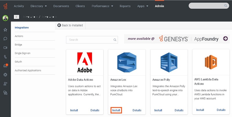
Integration consists of three simple steps (for full instructions, see About the Amazon Lex integration):
- Install the Amazon Lex integration from Genesys AppFoundry (Genesys Marketplace).
- Configure the IAM role with permissions for Amazon Lex.
- Set up and activate the Lex integration into Genesys Cloud.
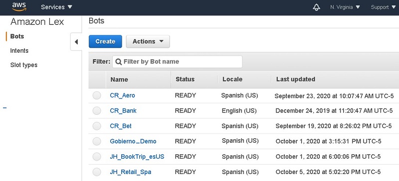
After completing these steps, you can use any bots that you configured in Amazon Lex within Genesys Cloud flows, regardless of whether the flow is for voice (IVR type) or for digital channels like web chat, social networks, and messaging channels. The following screenshot shows a view of available bots for our use case on the Amazon Lex console.
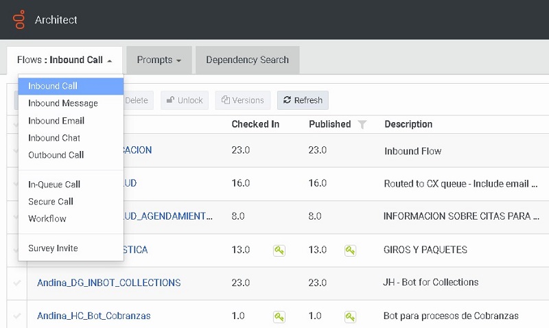
To use our sample retail management bot, go into Architect (a Genesys Cloud flow configuration product) and choose the type of flow to configure (voice, chat, or messaging) so you can use the tools available for that channel.
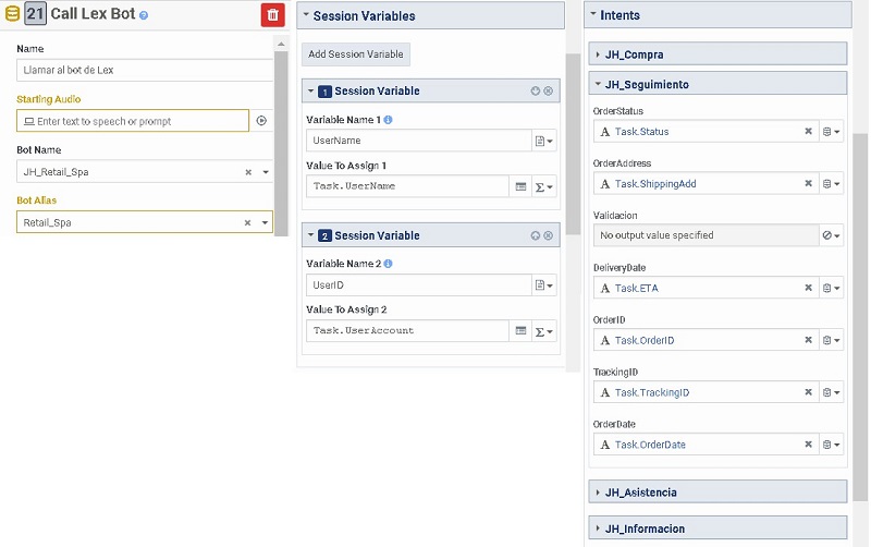
In the flow toolbox, you can add the Call Lex Bot action anywhere in the flow by adding it via drag-and-drop.

This is how you can call onto any of your existing Amazon Lex bots from a Genesys Cloud Architect flow. In this voice flow example, we first identify the customer through a query to the CRM before passing them to the bot.
The Call Lex Bot action allows you to select one of your existing bots and configure information to pass (input variables). It outputs the intent identified in Amazon Lex and the slot information collected by the bot (output variables). Genesys Cloud can use the outputs to continue processing the interaction and provide context to the human agent if the interaction is transferred.
Going back to our example, we use the bot JH_Retail_Spa and configure two variables to pass to Amazon Lex that we collected from the CRM earlier in the flow: Task.UserName and Task.UserAccount. We then configure the track an order intent and its associated output variables.
The output information is played back to the customer, who can choose to finish the interaction or, if necessary, seek the support of a human agent. The agent is presented with a script that provides them with the context so they can seamlessly pick up the conversation at the point where the bot left off. This means the customer avoids having to repeat themselves, removing friction and improving customer experience.
You can enable the same functionality on digital channels, such as web chat, social networks, or messaging applications like WhatsApp or Line. In this case, all you need to do is use the same Genesys Cloud Architect action (Call Lex Bot) in digital flows.
The following screenshot shows an example of interacting with a bot on an online shopping website.

As with voice calls, if the customer needs additional support in digital interactions, these interactions are transferred to agents according to the defined routing strategy. Again, context is provided and the transcription of the conversation between the client and the bot is displayed to the agent.

In addition to these use cases, you can use the Genesys Cloud REST API to generate additional interaction types, providing differentiated customer service. For example, with the release of Amazon Lex in Spanish, some of our customers and partners are building Alexa Skills, delivering an additional personalized communication channel to their users.
Conclusion
Customer experience operations are constantly coming up against new challenges, especially in the days of COVID-19. Genesys Cloud provides a solution that can manage all the changes we’re facing daily. It natively provides a flexible, agile, and resilient omni-channel solution that enables scalability on demand.
With the release of Amazon Lex in Spanish, you can quickly incorporate bots within your voice or digital channels, improving efficiency and customer service. These interactions can be transferred when needed to human agents with the proper context so they can continue the conversation seamlessly and focus on more complex cases where they can add more value.
If you have Genesys Cloud, check out the integration with Amazon Lex in Spanish and US Spanish to see how simple and beneficial it can be. If you’re not a customer, this is an additional reason to migrate and take full advantage of the benefits Genesys and AWS CCI can offer you. Differentiate your organization by personalizing every customer service interaction, improving agent satisfaction, and enhancing visibility into important business metrics with a more intelligent contact center.
About the Authors
Rebecca Owens is a Senior Product Manager at Genesys and is based out of Raleigh, North Carolina.
Julian Hernandez is Senior Cloud Business Development – LATAM for Genesys and is based out of Bogota D.C. Area, Colombia.

Amazon Transcribe streaming adds support for Japanese, Korean, and Brazilian Portuguese
Amazon Transcribe is an automatic speech recognition (ASR) service that makes it easy to add speech-to-text capabilities to your applications. Today, we’re excited to launch Japanese, Korean, and Brazilian Portuguese language support for Amazon Transcribe streaming. To deliver streaming transcriptions with low latency for these languages, we’re also announcing availability of Amazon Transcribe streaming in the Asia Pacific (Seoul), Asia Pacific (Tokyo), and South America (São Paulo) Regions.
Amazon Transcribe added support for Italian and German languages earlier in November 2020, and this launch continues to expand the service’s streaming footprint. Now you can automatically generate live streaming transcriptions for a diverse set of use cases within your contact centers and media production workflows.
Customer stories
Our customers are using Amazon Transcribe to capture customer calls in real time to better assist agents, improve call resolution times, generate content highlights on the fly, and more. Here are a few stories of their streaming audio use cases.
PLUS Corporation
PLUS Corporation is a global manufacturer and retailer of office supplies. Mr. Yoshiki Yamaguchi, the Deputy Director of the IT Department at PLUS, says, “Every day, our contact center processes millions of minutes of calls. We are excited by Amazon Transcribe’s new addition of Japanese language support for streaming audio. This will provide our agents and supervisors with a robust, streaming transcription service that will enable them to better analyze and monitor incoming calls to improve call handling times and customer service quality.”
Nomura Research Institute
Nomura Research Institute (NRI) is one of the largest economic research consulting firms in Japan and an AWS premier consulting partner specializing in contact center intelligence solutions. Mr. Kakinoki, the deputy division manager of NRI’s Digital Workplace Solutions says, “For decades, we have been bringing intelligence into contact centers by providing several Natural Language Processing (NLP) based solutions in Japanese. We are pleased to welcome Amazon Transcribe’s latest addition of Japanese support for streaming audio. This enables us to automatically provide agents with real-time call transcripts as part of our solution. Now we are able to offer an integrated AWS contact center solution to our customers that addresses their need for real-time FAQ knowledge recommendations and text summarization of inbound calls. This will help our customers such as large financial firms reduce call resolution times, increase agent productivity and improve quality management capabilities.”
Accenture
Dr. Gakuse Hoshina, a Managing Director and Lead for Japan Applied Intelligence at Accenture Strategy & Consulting, says, “Accenture provides services such as AI Powered Contact Center and AI Powered Concierge, which synergize automated AI responses and human interactions to help our clients create highly satisfying customer experiences. I expect that the latest addition of Japanese for Amazon Transcribe streaming support will lead to a further improved customer experience, improving the accuracy of AI’s information retrieval and automated responses.”
Audioburst
Audioburst is a technology provider that is transforming the discovery, distribution, and personalization of talk audio. Gal Klein, the co-founder and CTO of Audioburst, says, “Every day, we analyze 225,000 minutes of live talk radio to create thousands of short, topical segments of information for playlists and search. We chose Amazon Transcribe because it is a remarkable speech recognition engine that helps us transcribe live audio content for our downstream content production work streams. Transcribe provides a robust system that can simultaneously convert a hundred audio streams into text for a reasonable cost. With this high-quality output text, we are then able to quickly process live talk radio episodes into consumable segments that provide next-gen listening experiences and drive higher engagement.”
Getting started
You can try Amazon Transcribe streaming for any of these new languages on the Amazon Transcribe console. The following is a quick demo of how to use it in Japanese.
You can take advantage of streaming transcription within your own applications with the Amazon Transcribe API for HTTP/2 or WebSockets implementations.
For the full list of supported languages and Regions for Amazon Transcribe streaming, see Streaming Transcription and AWS Regional Services.
Summary
Amazon Transcribe is a powerful ASR service for accurately converting your real-time speech into text. Try using it to help streamline your content production needs and equip your agents with effective tools to improve your overall customer experience. See all the ways in which other customers are using Amazon Transcribe.
About the Author
 Esther Lee is a Product Manager for AWS Language AI Services. She is passionate about the intersection of technology and education. Out of the office, Esther enjoys long walks along the beach, dinners with friends and friendly rounds of Mahjong.
Real-time anomaly detection for Amazon Connect call quality using Amazon ES
If your contact center is serving calls over the internet, network metrics like packet loss, jitter, and round-trip time are key to understanding call quality. In the post Easily monitor call quality with Amazon Connect, we introduced a solution that captures real-time metrics from the Amazon Connect softphone, stores them in Amazon Elasticsearch Service (Amazon ES), and creates easily understandable dashboards using Kibana. Examining these metrics and implementing rule-based alerting can be valuable. However, as your contact center scales, outliers becomes harder to detect across broad aggregations. For example, average packet loss for each of your sites may be below a rule threshold, but individual agent issues might go undetected.
The high cardinality anomaly detection feature of Amazon ES is a machine learning (ML) approach that can solve this problem. You can streamline your operational workflows by detecting anomalies for individual agents across multiple metrics. Alerts allow you to proactively reach out to the agent to help them resolve issues as they’re detected or use the historical data in Amazon ES to understand the issue. In this post, we give a four-step guide to detecting an individual agent’s call quality anomalies.
Anomaly detection in four stages
If you have an Amazon Connect instance, you can deploy the solution and follow along with this post. There are four steps to getting started with using anomaly detection to proactively monitor your data:
- Create an anomaly detector.
- Observe the results.
- Configure alerts.
- Tune the detector.
Creating an anomaly detector
A detector is the component used to track anomalies in a data source in real time. Features are the metrics the detector monitors in that data.
Our solution creates a call quality metric detector when deployed. This detector finds potential call quality issues by monitoring network metrics for agents’ calls, with features for round trip time, packet loss, and jitter. We use high cardinality anomaly detection to monitor anomalies across these features and identify agents who are having issues. Getting these granular results means that you can effectively isolate trends or individual issues in your call center.
Observing results
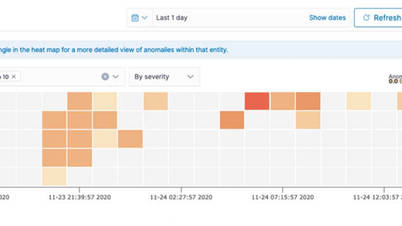
We can observe active detectors from Kibana’s anomaly detection dashboard. The graphs in Kibana show live anomalies, historical anomalies, and your feature data. You can determine the severity of an anomaly by the anomaly grade and the confidence of the detector. The following screenshot shows a heat map of anomalies detected, including the anomaly grade, confidence level, and the agents impacted.

We can choose any of the tiles in the heat map to drill down further and use the feature breakdown tab to see more details. For example, the following screenshot shows the feature breakdown of one the tiles from the agent john-doe. The feature breakdown shows us that the round trip time, jitter, and packet loss values spiked during this time period.

To see if this is an intermittent issue for this agent, we have two approaches. First, we can check the anomaly occurrences for the agent to see if there is a trend. In the following screenshot, John Doe had 12 anomalies over the last day, starting around 3:25 PM. This is a clear sign to investigate.

Alternatively, referencing the heat map, we can look to see if there is a visual trend. Our preceding heat map shows a block of anomalies around 9:40 PM on November 23—this is a reason to look at other broader issues impacting these agents. For instance, they might all be at the same site, which suggests we should look at the site’s network health.
Configuring alerts
We can also configure each detector with alerts to send a message to Amazon Chime or Slack. Alternatively, you can send alerts to an Amazon Simple Notification Service (Amazon SNS) topic for emails or SMS. Alerting an operations engineer or operations team allows you to investigate these issues in real time. For instructions on configuring these alerts, see Alerting for Amazon Elasticsearch Service.
Tuning the detector
It’s simple to start monitoring new features. You can add them to your model with a few clicks. To get the best results from your data, you can tailor the time window to your business. These time intervals are referred to as window size. The window size effects how quickly the algorithm adjusts to your data. Tuning the window size to match your data allows you to improve detector performance. For more information, see Anomaly Detection for Amazon Elasticsearch Service.
Conclusion
In this post, we’ve shown the value of high cardinality anomaly detection for Amazon ES. To get actionable insights and preconfigured anomaly detection for Amazon Connect metrics, you can deploy the call quality monitoring solution.
The high cardinality anomaly detection feature is available on all Amazon ES domains running Elasticsearch 7.9 or greater. For more information, see Anomaly Detection for Amazon Elasticsearch Service.
About the Authors
 Kun Qian is a Specialist Solutions Architect on the Amazon Connect Customer Solutions Acceleration team. He solving complex problems with technology. In his spare time he loves hiking, experimenting in the kitchen and meeting new people.
 Rob Taylor is a Solutions Architect helping customers in Australia designing and building solutions on AWS. He has a background in theoretical computer science and modeling. Originally from the US, in his spare time he enjoys exploring Australia and spending time with his family.

TensorFlow Recommenders: Scalable retrieval and feature interaction modelling
 Posted by Ruoxi Wang, Phil Sun, Rakesh Shivanna and Maciej Kula (Google)
In September, we open-sourced TensorFlow Recommenders, a library that makes building state-of-the-art recommender system models easy. Today, we’re excited to announce a new release of TensorFlow Recommenders (TFRS), v0.3.0.
The new version brings two important features, both critical to building and deploying high-quality, scalable recommender models.
The first is built-in support for fast, scalable approximate retrieval. By leveraging ScaNN, TFRS now makes it possible to build deep learning recommender models that can retrieve the best candidates out of millions in milliseconds – all while retaining the simplicity of deploying a single “query features in, recommendations out” SavedModel object.
The second is support for better techniques for modelling feature interactions. The new release of TFRS includes an implementation of Deep & Cross Network: efficient architectures for learning interactions between all the different features used in a deep learning recommender model.
If you’re eager to try out the new features, you can jump straight into our efficient retrieval and feature interaction modelling tutorials. Otherwise, read on to learn more!
Efficient retrieval
The goal of many recommender systems is to retrieve a handful of good recommendations out of a pool of millions or tens of millions of candidates. The retrieval stage of a recommender system tackles the “needle in a haystack” problem of finding a short list of promising candidates out of the entire candidate list.
As discussed in our previous blog post, TensorFlow Recommenders makes it easy to build two-tower retrieval models. Such models perform retrieval in two steps:
- Mapping user input to an embedding
- Finding the top candidates in embedding space
The cost of the first step is largely determined by the complexity of the query tower model. For example, if the user input is text, a query tower that uses an 8-layer transformer will be roughly twice as expensive to compute as one that uses a 4-layer transformer. Techniques such as sparsity, quantization, and architecture optimization all help with reducing this cost.
However, for large databases with millions of candidates, the second step is generally even more important for fast inference. Our two-tower model uses the dot product of the user input and candidate embedding to compute candidate relevancy, and although computing dot products is relatively cheap, computing one for every embedding in a database, which scales linearly with database size, quickly becomes computationally infeasible. A fast nearest neighbor search (NNS) algorithm is therefore crucial for recommender system performance.
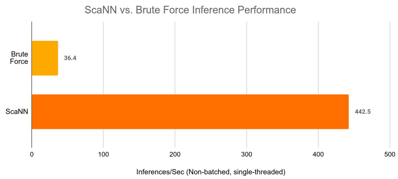
Enter ScaNN. ScaNN is a state-of-the-art NNS library from Google Research. It significantly outperforms other NNS libraries on standard benchmarks. Furthermore, it integrates seamlessly with TensorFlow Recommenders. As seen below, the ScaNN Keras layer acts as a seamless drop-in replacement for brute force retrieval:
# Create a model that takes in raw query features, and
# recommends movies out of the entire movies dataset.
# Before
# index = tfrs.layers.factorized_top_k.BruteForce(model.user_model)
# index.index(movies.batch(100).map(model.movie_model), movies)
# After
scann = tfrs.layers.factorized_top_k.ScaNN(model.user_model)
scann.index(movies.batch(100).map(model.movie_model), movies)

# Get recommendations.
# Before
# _, titles = index(tf.constant(["42"]))
# After
_, titles = scann(tf.constant(["42"]))
print(f"Recommendations for user 42: {titles[0, :3]}")
Because it’s a Keras layer, the ScaNN index serializes and automatically stays in sync with the rest of the TensorFlow Recommender model. There is also no need to shuttle requests back and forth between the model and ScaNN because everything is already wired up properly. As NNS algorithms improve, ScaNN’s efficiency will only improve and further improve retrieval accuracy and latency.
|
| ScaNN can speed up large retrieval models by over 10x while still providing almost the same retrieval accuracy as brute force vector retrieval. |
We believe that ScaNN’s features will lead to a transformational leap in the ease of deploying state-of-the-art deep retrieval models. If you’re interested in the details of how to build and serve ScaNN based models, have a look at our tutorial.
Deep cross networks
Effective feature crosses are the key to the success of many prediction models. Imagine that we are building a recommender system to sell blenders using users’ past purchase history. Individual features such as the number of bananas and cookbooks purchased give us some information about the user’s intent, but it is their combination – having bought both bananas and cookbooks – that gives us the strongest signal of the likelihood that the user will buy a blender. This combination of features is referred to as a feature cross.

In web-scale applications, data are mostly categorical, leading to large and sparse feature space. Identifying effective feature crosses in this setting often requires manual feature engineering or exhaustive search. Traditional feed-forward multilayer perceptron (MLP) models are universal function approximators; however, they cannot efficiently approximate even 2nd or 3rd-order feature crosses as pointed out in the Deep & Cross Network and Latent Cross papers.
What is a Deep & Cross Network (DCN)?
DCN was designed to learn explicit and bounded-degree cross features more effectively. They start with an input layer (typically an embedding layer), followed by a cross network which models explicit feature interactions, and finally a deep network that models implicit feature interactions.
Cross Network
This is the core of a DCN. It explicitly applies feature crossing at each layer, and the highest polynomial degree (feature cross order) increases with layer depth. The following figure shows the (𝑖+1)-th cross layer.
 |
| Cross layer visualization. x0 is the base layer (typically set as the embedding layer), xi is the input to the cross layer, ☉ represents element-wise multiplications, and matrix W and vector b are the parameters to be learned. |
When we only have a single cross layer, it creates 2nd-order (pairwise) feature crosses among input features. In the blender example above, the input to the cross layer would be a vector that concatenates three features: [country, purchased_bananas, purchased_cookbooks]. Then, the first dimension of the output would contain a weighted sum of pairwise interactions between country and all the three input features; the second dimension would contain weighted interactions of purchased_bananas and all the other features, and so on.
The weights of these interaction terms form the matrix W: if an interaction is unimportant, its weight will be close to zero. If it is important, it will be away from zero.
To create higher-order feature crosses, we could stack more cross layers. For example, we now know that a single cross layer outputs 2nd-order feature crosses such as interaction between purchased_bananas and purchased_cookbook. We could further feed these 2nd-order crosses to another cross layer. Then, the feature crossing part would multiply those 2nd-order crosses with the original (1st-order) features to create 3rd-order feature crosses, e.g., interactions among countries, purchased_bananas and purchased_cookbooks. The residual connection would carry over those feature crosses that have already been created in the previous layer.
If we stack k cross layers together, the k-layered cross network would create all the feature crosses up to order k+1, with their importance characterized by parameters in the weight matrices and bias vectors.
Deep Network
The deep part of a Deep & Cross Network is a traditional feedforward multilayer perceptron (MLP).
The deep network and cross network are then combined to form DCN. Commonly, we could stack a deep network on top of the cross network (stacked structure); we could also place them in parallel (parallel structure).
 |
| Deep & Cross Network (DCN) visualization. Left: parallel structure; Right: stacked structure. |
Model Understanding
A good understanding of the learned feature crosses helps improve model understandability. Fortunately, the weight matrix 𝑊 in the cross layer reveals what feature crosses the model has learned to be important.
Take the example of selling a blender to a customer. If purchasing both bananas and cookbooks is the most predictive signal in the data, a DCN model should be able to capture this relationship. The following figure shows the learned matrix of a DCN model with one cross layer, trained on synthetic data where the joint purchase feature is most important. We see that the model itself has learned that the interaction between `purchased_bananas` and `purchased_cookbooks` is important, without any manual feature engineering applied.
 |
| Learned weight matrix in the cross layer. |
Cross layers are now implemented in TensorFlow Recommenders, and you can easily adopt them as building blocks in your models. To learn how, check out our tutorial for example usage and practical lessons. If you are interested in more detail, have a look at our research papers DCN and DCN v2.
Acknowledgements
We would like to give a special thanks to Derek Zhiyuan Cheng, Sagar Jain, Shirley Zhe Chen, Dong Lin, Lichan Hong, Ed H. Chi, Bin Fu, Gang (Thomas) Fu and Mingliang Wang for their critical contributions to Deep & Cross Network (DCN). We also would like to thank everyone who has helped with and supported the DCN effort from research idea to productionization: Shawn Andrews, Sugato Basu, Jakob Bauer, Nick Bridle, Gianni Campion, Jilin Chen, Ting Chen, James Chen, Tianshuo Deng, Evan Ettinger, Eu-Jin Goh, Vidur Goyal, Julian Grady, Gary Holt, Samuel Ieong, Asif Islam, Tom Jablin, Jarrod Kahn, Duo Li, Yang Li, Albert Liang, Wenjing Ma, Aniruddh Nath, Todd Phillips, Ardian Poernomo, Kevin Regan, Olcay Sertel, Anusha Sriraman, Myles Sussman, Zhenyu Tan, Jiaxi Tang, Yayang Tian, Jason Trader, Tatiana Veremeenko, Jingjing Wang, Li Wei, Cliff Young, Shuying Zhang, Jie (Jerry) Zhang, Jinyin Zhang, Zhe Zhao and many more (in alphabetical order). We’d also like to thank David Simcha, Erik Lindgren, Felix Chern, Nathan Cordeiro, Ruiqi Guo, Sanjiv Kumar, Sebastian Claici, and Zonglin Li for their contributions to ScaNN.
Analyzing data stored in Amazon DocumentDB (with MongoDB compatibility) using Amazon Sagemaker
One of the challenges in data science is getting access to operational or real-time data, which is often stored in operational database systems. Being able to connect data science tools to operational data easily and efficiently unleashes enormous potential for gaining insights from real-time data. In this post, we explore using Amazon SageMaker to analyze data stored in Amazon DocumentDB (with MongoDB compatibility).
For illustrative purposes, we use public event data from the GitHub API, which has a complex nested JSON format, and is well-suited for a document database such as Amazon DocumentDB. We use SageMaker to analyze this data, conduct descriptive analysis, and build a simple machine learning (ML) model to predict whether a pull request will close within 24 hours, before writing prediction results back into the database.
SageMaker is a fully managed service that provides every developer and data scientist with the ability to build, train, and deploy ML models quickly. SageMaker removes the heavy lifting from each step of the ML process to make it easier to develop high-quality models.
Amazon DocumentDB is a fast, scalable, highly available, and fully managed document database service that supports MongoDB workloads. You can use the same MongoDB 3.6 application code, drivers, and tools to run, manage, and scale workloads on Amazon DocumentDB without having to worry about managing the underlying infrastructure. As a document database, Amazon DocumentDB makes it easy to store, query, and index JSON data.
Solution overview
In this post, we analyze GitHub events, examples of which include issues, forks, and pull requests. Each event is represented by the GitHub API as a complex, nested JSON object, which is a format well-suited for Amazon DocumentDB. The following code is an example of the output from a pull request event:
{
  "id": "13469392114",
  "type": "PullRequestEvent",
  "actor": {
    "id": 33526713,
    "login": "arjkesh",
    "display_login": "arjkesh",
    "gravatar_id": "",
    "url": "https://api.github.com/users/arjkesh",
    "avatar_url": "https://avatars.githubusercontent.com/u/33526713?"
  },
  "repo": {
    "id": 234634164,
    "name": "aws/deep-learning-containers",
    "url": "https://api.github.com/repos/aws/deep-learning-containers"
  },
  "payload": {
    "action": "closed",
    "number": 570,
    "pull_request": {
      "url": "https://api.github.com/repos/aws/deep-learning-containers/pulls/570",
      "id": 480316742,
      "node_id": "MDExOlB1bGxSZXF1ZXN0NDgwMzE2NzQy",
      "html_url": "https://github.com/aws/deep-learning-containers/pull/570",
      "diff_url": "https://github.com/aws/deep-learning-containers/pull/570.diff",
      "patch_url": "https://github.com/aws/deep-learning-containers/pull/570.patch",
      "issue_url": "https://api.github.com/repos/aws/deep-learning-containers/issues/570",
      "number": 570,
      "state": "closed",
      "locked": false,
      "title": "[test][tensorflow][ec2] Add timeout to Data Service test setup",
      "user": {
        "login": "arjkesh",
        "id": 33526713,
        "node_id": "MDQ6VXNlcjMzNTI2NzEz",
        "avatar_url": "https://avatars3.githubusercontent.com/u/33526713?v=4",
        "gravatar_id": "",
        "url": "https://api.github.com/users/arjkesh",
        "html_url": "https://github.com/arjkesh",
        "followers_url": "https://api.github.com/users/arjkesh/followers",
        "following_url": "https://api.github.com/users/arjkesh/following{/other_user}",
        "gists_url": "https://api.github.com/users/arjkesh/gists{/gist_id}",
        "starred_url": "https://api.github.com/users/arjkesh/starred{/owner}{/repo}",
        "subscriptions_url": "https://api.github.com/users/arjkesh/subscriptions",
        "organizations_url": "https://api.github.com/users/arjkesh/orgs",
        "repos_url": "https://api.github.com/users/arjkesh/repos",
        "events_url": "https://api.github.com/users/arjkesh/events{/privacy}",
        "received_events_url": "https://api.github.com/users/arjkesh/received_events",
        "type": "User",
        "site_admin": false
      },
      "body": "*Issue #, if available:*rnrn## Checklistrn- [x] I've prepended PR tag with frameworks/job this applies to : [mxnet, tensorflow, pytorch] | [ei/neuron] | [build] | [test] | [benchmark] | [ec2, ecs, eks, sagemaker]rnrn*Description:*rnCurrently, this test does not timeout in the same manner as execute_ec2_training_test or other ec2 training tests. As such, a timeout should be added here to avoid hanging instances. A separate PR will be opened to address why the global timeout does not catch this.rnrn*Tests run:*rnPR testsrnrnrnBy submitting this pull request, I confirm that my contribution is made under the terms of the Apache 2.0 license. I confirm that you can use, modify, copy, and redistribute this contribution, under the terms of your choice.rnrn",
      "created_at": "2020-09-05T00:29:22Z",
      "updated_at": "2020-09-10T06:16:53Z",
      "closed_at": "2020-09-10T06:16:53Z",
      "merged_at": null,
      "merge_commit_sha": "4144152ac0129a68c9c6f9e45042ecf1d89d3e1a",
      "assignee": null,
      "assignees": [

      ],
      "requested_reviewers": [

      ],
      "requested_teams": [

      ],
      "labels": [

      ],
      "milestone": null,
      "draft": false,
      "commits_url": "https://api.github.com/repos/aws/deep-learning-containers/pulls/570/commits",
      "review_comments_url": "https://api.github.com/repos/aws/deep-learning-containers/pulls/570/comments",
      "review_comment_url": "https://api.github.com/repos/aws/deep-learning-containers/pulls/comments{/number}",
      "comments_url": "https://api.github.com/repos/aws/deep-learning-containers/issues/570/comments",
      "statuses_url": "https://api.github.com/repos/aws/deep-learning-containers/statuses/99bb5a14993ceb29c16641bd54865db46ee6bf59",
      "head": {
        "label": "arjkesh:add_timeouts",
        "ref": "add_timeouts",
        "sha": "99bb5a14993ceb29c16641bd54865db46ee6bf59",
        "user": {
          "login": "arjkesh",
          "id": 33526713,
          "node_id": "MDQ6VXNlcjMzNTI2NzEz",
          "avatar_url": "https://avatars3.githubusercontent.com/u/33526713?v=4",
          "gravatar_id": "",
          "url": "https://api.github.com/users/arjkesh",
          "html_url": "https://github.com/arjkesh",
          "followers_url": "https://api.github.com/users/arjkesh/followers",
          "following_url": "https://api.github.com/users/arjkesh/following{/other_user}",
          "gists_url": "https://api.github.com/users/arjkesh/gists{/gist_id}",
          "starred_url": "https://api.github.com/users/arjkesh/starred{/owner}{/repo}",
          "subscriptions_url": "https://api.github.com/users/arjkesh/subscriptions",
          "organizations_url": "https://api.github.com/users/arjkesh/orgs",
          "repos_url": "https://api.github.com/users/arjkesh/repos",
          "events_url": "https://api.github.com/users/arjkesh/events{/privacy}",
          "received_events_url": "https://api.github.com/users/arjkesh/received_events",
          "type": "User",
          "site_admin": false
        },
        "repo": {
          "id": 265346646,
          "node_id": "MDEwOlJlcG9zaXRvcnkyNjUzNDY2NDY=",
          "name": "deep-learning-containers-1",
          "full_name": "arjkesh/deep-learning-containers-1",
          "private": false,
          "owner": {
            "login": "arjkesh",
            "id": 33526713,
            "node_id": "MDQ6VXNlcjMzNTI2NzEz",
            "avatar_url": "https://avatars3.githubusercontent.com/u/33526713?v=4",
            "gravatar_id": "",
            "url": "https://api.github.com/users/arjkesh",
            "html_url": "https://github.com/arjkesh",
            "followers_url": "https://api.github.com/users/arjkesh/followers",
            "following_url": "https://api.github.com/users/arjkesh/following{/other_user}",
            "gists_url": "https://api.github.com/users/arjkesh/gists{/gist_id}",
            "starred_url": "https://api.github.com/users/arjkesh/starred{/owner}{/repo}",
            "subscriptions_url": "https://api.github.com/users/arjkesh/subscriptions",
            "organizations_url": "https://api.github.com/users/arjkesh/orgs",
            "repos_url": "https://api.github.com/users/arjkesh/repos",
            "events_url": "https://api.github.com/users/arjkesh/events{/privacy}",
            "received_events_url": "https://api.github.com/users/arjkesh/received_events",
            "type": "User",
            "site_admin": false
          },
          "html_url": "https://github.com/arjkesh/deep-learning-containers-1",
          "description": "AWS Deep Learning Containers (DLCs) are a set of Docker images for training and serving models in TensorFlow, TensorFlow 2, PyTorch, and MXNet.",
          "fork": true,
          "url": "https://api.github.com/repos/arjkesh/deep-learning-containers-1",
          "forks_url": "https://api.github.com/repos/arjkesh/deep-learning-containers-1/forks",
          "keys_url": "https://api.github.com/repos/arjkesh/deep-learning-containers-1/keys{/key_id}",
          "collaborators_url": "https://api.github.com/repos/arjkesh/deep-learning-containers-1/collaborators{/collaborator}",
          "teams_url": "https://api.github.com/repos/arjkesh/deep-learning-containers-1/teams",
          "hooks_url": "https://api.github.com/repos/arjkesh/deep-learning-containers-1/hooks",
          "issue_events_url": "https://api.github.com/repos/arjkesh/deep-learning-containers-1/issues/events{/number}",
          "events_url": "https://api.github.com/repos/arjkesh/deep-learning-containers-1/events",
          "assignees_url": "https://api.github.com/repos/arjkesh/deep-learning-containers-1/assignees{/user}",
          "branches_url": "https://api.github.com/repos/arjkesh/deep-learning-containers-1/branches{/branch}",
          "tags_url": "https://api.github.com/repos/arjkesh/deep-learning-containers-1/tags",
          "blobs_url": "https://api.github.com/repos/arjkesh/deep-learning-containers-1/git/blobs{/sha}",
          "git_tags_url": "https://api.github.com/repos/arjkesh/deep-learning-containers-1/git/tags{/sha}",
          "git_refs_url": "https://api.github.com/repos/arjkesh/deep-learning-containers-1/git/refs{/sha}",
          "trees_url": "https://api.github.com/repos/arjkesh/deep-learning-containers-1/git/trees{/sha}",
          "statuses_url": "https://api.github.com/repos/arjkesh/deep-learning-containers-1/statuses/{sha}",
          "languages_url": "https://api.github.com/repos/arjkesh/deep-learning-containers-1/languages",
          "stargazers_url": "https://api.github.com/repos/arjkesh/deep-learning-containers-1/stargazers",
          "contributors_url": "https://api.github.com/repos/arjkesh/deep-learning-containers-1/contributors",
          "subscribers_url": "https://api.github.com/repos/arjkesh/deep-learning-containers-1/subscribers",
          "subscription_url": "https://api.github.com/repos/arjkesh/deep-learning-containers-1/subscription",
          "commits_url": "https://api.github.com/repos/arjkesh/deep-learning-containers-1/commits{/sha}",
          "git_commits_url": "https://api.github.com/repos/arjkesh/deep-learning-containers-1/git/commits{/sha}",
          "comments_url": "https://api.github.com/repos/arjkesh/deep-learning-containers-1/comments{/number}",
          "issue_comment_url": "https://api.github.com/repos/arjkesh/deep-learning-containers-1/issues/comments{/number}",
          "contents_url": "https://api.github.com/repos/arjkesh/deep-learning-containers-1/contents/{+path}",
          "compare_url": "https://api.github.com/repos/arjkesh/deep-learning-containers-1/compare/{base}...{head}",
          "merges_url": "https://api.github.com/repos/arjkesh/deep-learning-containers-1/merges",
          "archive_url": "https://api.github.com/repos/arjkesh/deep-learning-containers-1/{archive_format}{/ref}",
          "downloads_url": "https://api.github.com/repos/arjkesh/deep-learning-containers-1/downloads",
          "issues_url": "https://api.github.com/repos/arjkesh/deep-learning-containers-1/issues{/number}",
          "pulls_url": "https://api.github.com/repos/arjkesh/deep-learning-containers-1/pulls{/number}",
          "milestones_url": "https://api.github.com/repos/arjkesh/deep-learning-containers-1/milestones{/number}",
          "notifications_url": "https://api.github.com/repos/arjkesh/deep-learning-containers-1/notifications{?since,all,participating}",
          "labels_url": "https://api.github.com/repos/arjkesh/deep-learning-containers-1/labels{/name}",
          "releases_url": "https://api.github.com/repos/arjkesh/deep-learning-containers-1/releases{/id}",
          "deployments_url": "https://api.github.com/repos/arjkesh/deep-learning-containers-1/deployments",
          "created_at": "2020-05-19T19:38:21Z",
          "updated_at": "2020-06-23T04:18:45Z",
          "pushed_at": "2020-09-10T02:04:27Z",
          "git_url": "git://github.com/arjkesh/deep-learning-containers-1.git",
          "ssh_url": "git@github.com:arjkesh/deep-learning-containers-1.git",
          "clone_url": "https://github.com/arjkesh/deep-learning-containers-1.git",
          "svn_url": "https://github.com/arjkesh/deep-learning-containers-1",
          "homepage": "https://docs.aws.amazon.com/deep-learning-containers/latest/devguide/deep-learning-containers-images.html",
          "size": 68734,
          "stargazers_count": 0,
          "watchers_count": 0,
          "language": "Python",
          "has_issues": false,
          "has_projects": true,
          "has_downloads": true,
          "has_wiki": true,
          "has_pages": true,
          "forks_count": 0,
          "mirror_url": null,
          "archived": false,
          "disabled": false,
          "open_issues_count": 0,
          "license": {
            "key": "apache-2.0",
            "name": "Apache License 2.0",
            "spdx_id": "Apache-2.0",
            "url": "https://api.github.com/licenses/apache-2.0",
            "node_id": "MDc6TGljZW5zZTI="
          },
          "forks": 0,
          "open_issues": 0,
          "watchers": 0,
          "default_branch": "master"
        }
      },
      "base": {
        "label": "aws:master",
        "ref": "master",
        "sha": "9514fde23ae9eeffb9dfba13ce901fafacef30b5",
        "user": {
          "login": "aws",
          "id": 2232217,
          "node_id": "MDEyOk9yZ2FuaXphdGlvbjIyMzIyMTc=",
          "avatar_url": "https://avatars3.githubusercontent.com/u/2232217?v=4",
          "gravatar_id": "",
          "url": "https://api.github.com/users/aws",
          "html_url": "https://github.com/aws",
          "followers_url": "https://api.github.com/users/aws/followers",
          "following_url": "https://api.github.com/users/aws/following{/other_user}",
          "gists_url": "https://api.github.com/users/aws/gists{/gist_id}",
          "starred_url": "https://api.github.com/users/aws/starred{/owner}{/repo}",
          "subscriptions_url": "https://api.github.com/users/aws/subscriptions",
          "organizations_url": "https://api.github.com/users/aws/orgs",
          "repos_url": "https://api.github.com/users/aws/repos",
          "events_url": "https://api.github.com/users/aws/events{/privacy}",
          "received_events_url": "https://api.github.com/users/aws/received_events",
          "type": "Organization",
          "site_admin": false
        },
        "repo": {
          "id": 234634164,
          "node_id": "MDEwOlJlcG9zaXRvcnkyMzQ2MzQxNjQ=",
          "name": "deep-learning-containers",
          "full_name": "aws/deep-learning-containers",
          "private": false,
          "owner": {
            "login": "aws",
            "id": 2232217,
            "node_id": "MDEyOk9yZ2FuaXphdGlvbjIyMzIyMTc=",
            "avatar_url": "https://avatars3.githubusercontent.com/u/2232217?v=4",
            "gravatar_id": "",
            "url": "https://api.github.com/users/aws",
            "html_url": "https://github.com/aws",
            "followers_url": "https://api.github.com/users/aws/followers",
            "following_url": "https://api.github.com/users/aws/following{/other_user}",
            "gists_url": "https://api.github.com/users/aws/gists{/gist_id}",
            "starred_url": "https://api.github.com/users/aws/starred{/owner}{/repo}",
            "subscriptions_url": "https://api.github.com/users/aws/subscriptions",
            "organizations_url": "https://api.github.com/users/aws/orgs",
            "repos_url": "https://api.github.com/users/aws/repos",
            "events_url": "https://api.github.com/users/aws/events{/privacy}",
            "received_events_url": "https://api.github.com/users/aws/received_events",
            "type": "Organization",
            "site_admin": false
          },
          "html_url": "https://github.com/aws/deep-learning-containers",
          "description": "AWS Deep Learning Containers (DLCs) are a set of Docker images for training and serving models in TensorFlow, TensorFlow 2, PyTorch, and MXNet.",
          "fork": false,
          "url": "https://api.github.com/repos/aws/deep-learning-containers",
          "forks_url": "https://api.github.com/repos/aws/deep-learning-containers/forks",
          "keys_url": "https://api.github.com/repos/aws/deep-learning-containers/keys{/key_id}",
          "collaborators_url": "https://api.github.com/repos/aws/deep-learning-containers/collaborators{/collaborator}",
          "teams_url": "https://api.github.com/repos/aws/deep-learning-containers/teams",
          "hooks_url": "https://api.github.com/repos/aws/deep-learning-containers/hooks",
          "issue_events_url": "https://api.github.com/repos/aws/deep-learning-containers/issues/events{/number}",
          "events_url": "https://api.github.com/repos/aws/deep-learning-containers/events",
          "assignees_url": "https://api.github.com/repos/aws/deep-learning-containers/assignees{/user}",
          "branches_url": "https://api.github.com/repos/aws/deep-learning-containers/branches{/branch}",
          "tags_url": "https://api.github.com/repos/aws/deep-learning-containers/tags",
          "blobs_url": "https://api.github.com/repos/aws/deep-learning-containers/git/blobs{/sha}",
          "git_tags_url": "https://api.github.com/repos/aws/deep-learning-containers/git/tags{/sha}",
          "git_refs_url": "https://api.github.com/repos/aws/deep-learning-containers/git/refs{/sha}",
          "trees_url": "https://api.github.com/repos/aws/deep-learning-containers/git/trees{/sha}",
          "statuses_url": "https://api.github.com/repos/aws/deep-learning-containers/statuses/{sha}",
          "languages_url": "https://api.github.com/repos/aws/deep-learning-containers/languages",
          "stargazers_url": "https://api.github.com/repos/aws/deep-learning-containers/stargazers",
          "contributors_url": "https://api.github.com/repos/aws/deep-learning-containers/contributors",
          "subscribers_url": "https://api.github.com/repos/aws/deep-learning-containers/subscribers",
          "subscription_url": "https://api.github.com/repos/aws/deep-learning-containers/subscription",
          "commits_url": "https://api.github.com/repos/aws/deep-learning-containers/commits{/sha}",
          "git_commits_url": "https://api.github.com/repos/aws/deep-learning-containers/git/commits{/sha}",
          "comments_url": "https://api.github.com/repos/aws/deep-learning-containers/comments{/number}",
          "issue_comment_url": "https://api.github.com/repos/aws/deep-learning-containers/issues/comments{/number}",
          "contents_url": "https://api.github.com/repos/aws/deep-learning-containers/contents/{+path}",
          "compare_url": "https://api.github.com/repos/aws/deep-learning-containers/compare/{base}...{head}",
          "merges_url": "https://api.github.com/repos/aws/deep-learning-containers/merges",
          "archive_url": "https://api.github.com/repos/aws/deep-learning-containers/{archive_format}{/ref}",
          "downloads_url": "https://api.github.com/repos/aws/deep-learning-containers/downloads",
          "issues_url": "https://api.github.com/repos/aws/deep-learning-containers/issues{/number}",
          "pulls_url": "https://api.github.com/repos/aws/deep-learning-containers/pulls{/number}",
          "milestones_url": "https://api.github.com/repos/aws/deep-learning-containers/milestones{/number}",
          "notifications_url": "https://api.github.com/repos/aws/deep-learning-containers/notifications{?since,all,participating}",
          "labels_url": "https://api.github.com/repos/aws/deep-learning-containers/labels{/name}",
          "releases_url": "https://api.github.com/repos/aws/deep-learning-containers/releases{/id}",
          "deployments_url": "https://api.github.com/repos/aws/deep-learning-containers/deployments",
          "created_at": "2020-01-17T20:52:43Z",
          "updated_at": "2020-09-09T22:57:46Z",
          "pushed_at": "2020-09-10T04:01:22Z",
          "git_url": "git://github.com/aws/deep-learning-containers.git",
          "ssh_url": "git@github.com:aws/deep-learning-containers.git",
          "clone_url": "https://github.com/aws/deep-learning-containers.git",
          "svn_url": "https://github.com/aws/deep-learning-containers",
          "homepage": "https://docs.aws.amazon.com/deep-learning-containers/latest/devguide/deep-learning-containers-images.html",
          "size": 68322,
          "stargazers_count": 61,
          "watchers_count": 61,
          "language": "Python",
          "has_issues": true,
          "has_projects": true,
          "has_downloads": true,
          "has_wiki": true,
          "has_pages": false,
          "forks_count": 49,
          "mirror_url": null,
          "archived": false,
          "disabled": false,
          "open_issues_count": 28,
          "license": {
            "key": "apache-2.0",
            "name": "Apache License 2.0",
            "spdx_id": "Apache-2.0",
            "url": "https://api.github.com/licenses/apache-2.0",
            "node_id": "MDc6TGljZW5zZTI="
          },
          "forks": 49,
          "open_issues": 28,
          "watchers": 61,
          "default_branch": "master"
        }
      },
      "_links": {
        "self": {
          "href": "https://api.github.com/repos/aws/deep-learning-containers/pulls/570"
        },
        "html": {
          "href": "https://github.com/aws/deep-learning-containers/pull/570"
        },
        "issue": {
          "href": "https://api.github.com/repos/aws/deep-learning-containers/issues/570"
        },
        "comments": {
          "href": "https://api.github.com/repos/aws/deep-learning-containers/issues/570/comments"
        },
        "review_comments": {
          "href": "https://api.github.com/repos/aws/deep-learning-containers/pulls/570/comments"
        },
        "review_comment": {
          "href": "https://api.github.com/repos/aws/deep-learning-containers/pulls/comments{/number}"
        },
        "commits": {
          "href": "https://api.github.com/repos/aws/deep-learning-containers/pulls/570/commits"
        },
        "statuses": {
          "href": "https://api.github.com/repos/aws/deep-learning-containers/statuses/99bb5a14993ceb29c16641bd54865db46ee6bf59"
        }
      },
      "author_association": "CONTRIBUTOR",
      "active_lock_reason": null,
      "merged": false,
      "mergeable": false,
      "rebaseable": false,
      "mergeable_state": "dirty",
      "merged_by": null,
      "comments": 1,
      "review_comments": 0,
      "maintainer_can_modify": false,
      "commits": 6,
      "additions": 26,
      "deletions": 18,
      "changed_files": 1
    }
  },
  "public": true,
  "created_at": "2020-09-10T06:16:53Z",
  "org": {
    "id": 2232217,
    "login": "aws",
    "gravatar_id": "",
    "url": "https://api.github.com/orgs/aws",
    "avatar_url": "https://avatars.githubusercontent.com/u/2232217?"
  }
}
Amazon DocumentDB stores each JSON event as a document. Multiple documents are stored in a collection, and multiple collections are stored in a database. Borrowing terminology from relational databases, documents are analogous to rows, and collections are analogous to tables. The following table summarizes these terms.
| Document Database Concepts | SQL Concepts |
| Document | Row |
| Collection | Table |
| Database | Database |
| Field | Column |
We now implement the following Amazon DocumentDB tasks using SageMaker:
- Connect to an Amazon DocumentDB cluster.
- Ingest GitHub event data stored in the database.
- Generate descriptive statistics.
- Conduct feature selection and engineering.
- Generate predictions.
- Store prediction results.
Creating resources
We have prepared the following AWS CloudFormation template to create the required AWS resources for this post. For instructions on creating a CloudFormation stack, see the video Simplify your Infrastructure Management using AWS CloudFormation.
The CloudFormation stack provisions the following:
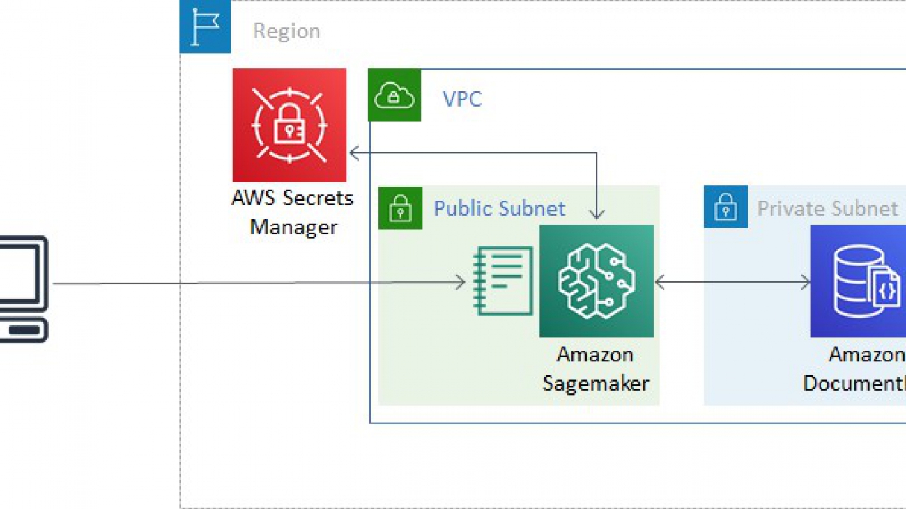
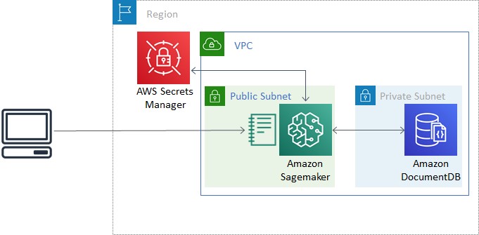
- A VPC with three private subnets and one public subnet.
- An Amazon DocumentDB cluster with three nodes, one in each private subnet. When creating an Amazon DocumentDB cluster in a VPC, its subnet group should have subnets in at least two Availability Zones in a given Region.
- An AWS Secrets Manager secret to store login credentials for Amazon DocumentDB. This allows us to avoid storing plaintext credentials in our SageMaker instance.
- A SageMaker role to retrieve the Amazon DocumentDB login credentials, allowing connections to the Amazon DocumentDB cluster from a SageMaker notebook.
- A SageMaker instance to run queries and analysis.
- A SageMaker instance lifecycle configuration to run a bash script every time the instance boots up, downloading a certificate bundle to create TLS connections to Amazon DocumentDB, as well as a Jupyter Notebook containing the code for this tutorial. The script also installs required Python libraries (such as
pymongofor database methods andxgboostfor ML modeling), so that we don’t need to install these libraries from the notebook. See the following code:#!/bin/bash sudo -u ec2-user -i <<'EOF' source /home/ec2-user/anaconda3/bin/activate python3 pip install --upgrade pymongo pip install --upgrade xgboost source /home/ec2-user/anaconda3/bin/deactivate cd /home/ec2-user/SageMaker wget https://s3.amazonaws.com/rds-downloads/rds-combined-ca-bundle.pem wget https://github.com/aws-samples/documentdb-sagemaker-example/blob/main/script.ipynb EOF
In creating the CloudFormation stack, you need to specify the following:
- Name for your CloudFormation stack
- Amazon DocumentDB username and password (to be stored in Secrets Manager)
- Amazon DocumentDB instance type (default db.r5.large)
- SageMaker instance type (default ml.t3.xlarge)
It should take about 15 minutes to create the CloudFormation stack. The following diagram shows the resource architecture.
Running this tutorial for an hour should cost no more than US$2.00.
Connecting to an Amazon DocumentDB cluster
All the subsequent code in this tutorial is in the Jupyter Notebook in the SageMaker instance created in your CloudFormation stack.
- To connect to your Amazon DocumentDB cluster from a SageMaker notebook, you have to first specify the following code:
stack_name = "docdb-sm" # name of CloudFormation stack
The stack_name refers to the name you specified for your CloudFormation stack upon its creation.
- Use this parameter in the following method to get your Amazon DocumentDB credentials stored in Secrets Manager:
def get_secret(stack_name):

    # Create a Secrets Manager client
    session = boto3.session.Session()
    client = session.client(
        service_name='secretsmanager',
        region_name=session.region_name
    )

    secret_name = f'{stack_name}-DocDBSecret'
    get_secret_value_response = client.get_secret_value(SecretId=secret_name)
    secret = get_secret_value_response['SecretString']

    return json.loads(secret)
- Next, we extract the login parameters from the stored secret:
secret = get_secret(secret_name)

db_username = secret['username']
db_password = secret['password']
db_port = secret['port']
db_host = secret['host']
- Using the extracted parameters, we create a
MongoClientfrom thepymongolibrary to establish a connection to the Amazon DocumentDB cluster.uri_str = f"mongodb://{db_username}:{db_password}@{db_host}:{db_port}/?ssl=true&ssl_ca_certs=rds-combined-ca-bundle.pem&replicaSet=rs0&readPreference=secondaryPreferred&retryWrites=false" client = MongoClient(uri_str)
Ingesting data
After we establish the connection to our Amazon DocumentDB cluster, we create a database and collection to store our GitHub event data. For this post, we name our database gharchive, and our collection events:
db_name = "gharchive" # name the database
collection_name = "events" # name the collection

db = client[db_name] # create a database
events = db[collection_name] # create a collection
Next, we need to download the data from gharchive.org, which has been aggregated into hourly archives with the following naming format:
https://data.gharchive.org/YYYY-MM-DD-H.json.gz
The aim of this analysis is to predict whether a pull request closes within 24 hours. For simplicity, we limit the analysis over two days: February 10–11, 2015. Across these two days, there were over 1 million GitHub events.
The following code downloads the relevant hourly archives, then formats and ingests the data into your Amazon DocumentDB database. It takes about 7 minutes to run on an ml.t3.xlarge instance.
# Specify target date and time range for GitHub events
year = 2015
month = 2
days = [10, 11]
hours = range(0, 24)

# Download data from gharchive.org and insert into Amazon DocumentDB

for day in days:
    for hour in hours:

        print(f"Processing events for {year}-{month}-{day}, {hour} hr.")

        # zeropad values
        month_ = str(month).zfill(2)
        day_ = str(day).zfill(2)

        # download data
        url = f"https://data.gharchive.org/{year}-{month_}-{day_}-{hour}.json.gz"
        response = requests.get(url, stream=True)

        # decompress data
        respdata = zlib.decompress(response.content, zlib.MAX_WBITS|32)

        # format data
        stringdata = respdata.split(b'n')
        data = [json.loads(x) for x in stringdata if 0 < len(x)]

        # ingest data
        events.insert_many(data, ordered=True, bypass_document_validation=True)
The option ordered=False command allows the data to be ingested out of order. The bypass_document_validation=True command allows the write to skip validating the JSON input, which is safe to do because we validated the JSON structure when we issued the json.loads() command prior to inserting.
Both options expedite the data ingestion process.
Generating descriptive statistics
As is a common first step in data science, we want to explore the data to get some general descriptive statistics. We can use database operations to calculate some of these basic descriptive statistics.
To get a count of the number of GitHub events, we use the count_documents() command:
events.count_documents({})
> 1174157
The count_documents() command gets the number of documents in a collection. Each GitHub event is recorded as a document, and events is what we had named our collection earlier.
The 1,174,157 documents comprise different types of GitHub events. To see the frequency of each type of event occurring in the dataset, we query the database using the aggregate command:
# Frequency of event types
event_types_query = events.aggregate([
    # Group by the type attribute and count
    {"$group" : {"_id": "$type", "count": {"$sum": 1}}},
    # Reformat the data
    {"$project": {"_id": 0, "Type": "$_id", "count": "$count"}},
    # Sort by the count in descending order
    {"$sort": {"count": -1} }
])
df_event_types = pd.DataFrame(event_types_query
The preceding query groups the events by type, runs a count, and sorts the results in descending order of count. Finally, we wrap the output in pd.DataFrame() to convert the results to a DataFrame. This allows us to generate visualizations such as the following.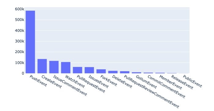
From the plot, we can see that push events were the most frequent, numbering close to 600,000.
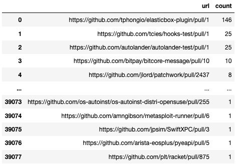
Returning to our goal to predict if a pull request closes within 24 hours, we implement another query to include only pull request events, using the database match operation, and then count the number of such events per pull request URL:
# Frequency of PullRequestEvent actions by URL
action_query = events.aggregate([
    # Keep only PullRequestEvent types
    {"$match" : {"type": "PullRequestEvent"} },
    # Group by HTML URL and count
    {"$group": {"_id": "$payload.pull_request.html_url", "count": {"$sum": 1}}},
    # Reformat the data
    {"$project": {"_id": 0, "url": "$_id", "count": "$count"}},
    # Sort by the count in descending order
    {"$sort": {"count": -1} }
])
df_action = pd.DataFrame(action_query)
From the result, we can see that a single URL could have multiple pull request events, such as those shown in the following screenshot.
One of the attributes of a pull request event is the state of the pull request after the event. Therefore, we’re interested in the latest event by the end of 24 hours in determining whether the pull request was open or closed in that window of time. We show how to run this query later in this post, but continue now with a discussion of descriptive statistics.
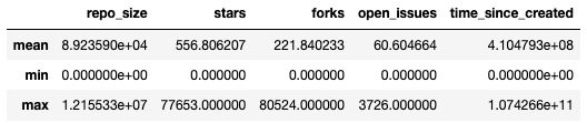
Apart from counts, we can also have the database calculate the mean, maximum, and minimum values for us. In the following query, we do this for potential predictors of a pull request open/close status, specifically the number of stars, forks, and open issues, as well as repository size. We also calculate the time elapsed (in milliseconds) of a pull request event since its creation. For each pull request, there could be multiple pull request events (comments), and this descriptive query spans across all these events:
# Descriptive statistics (mean, max, min) of repo size, stars, forks, open issues, elapsed time
descriptives = list(events.aggregate([
    # Keep only PullRequestEvents
    {"$match": {"type": "PullRequestEvent"} },
    # Project out attributes of interest
    {"$project": {
        "_id": 0,
        "repo_size": "$payload.pull_request.base.repo.size",
        "stars": "$payload.pull_request.base.repo.stargazers_count",
        "forks": "$payload.pull_request.base.repo.forks_count",
        "open_issues": "$payload.pull_request.base.repo.open_issues_count",
        "time_since_created": {"$subtract": [{"$dateFromString": {"dateString": "$payload.pull_request.updated_at"}},
                                  {"$dateFromString": {"dateString": "$payload.pull_request.created_at"}}]}
    }},
    # Calculate min/max/avg for various metrics grouped over full data set
    {"$group": {
        "_id": "descriptives",
        "mean_repo_size": {"$avg": "$repo_size"},
        "mean_stars": {"$avg": "$stars"},
        "mean_forks": {"$avg": "$forks"},
        "mean_open_issues": {"$avg": "$open_issues" },
        "mean_time_since_created": {"$avg": "$time_since_created"},

        "min_repo_size": {"$min": "$repo_size"},
        "min_stars": {"$min": "$stars"},
        "min_forks": {"$min": "$forks"},
        "min_open_issues": {"$min": "$open_issues" },
        "min_time_since_created": {"$min": "$time_since_created"},

        "max_repo_size": {"$max": "$repo_size"},
        "max_stars": {"$max": "$stars"},
        "max_forks": {"$max": "$forks"},
        "max_open_issues": {"$max": "$open_issues" },
        "max_time_since_created": {"$max": "$time_since_created"}
    }},
    # Reformat results
    {"$project": {
        "_id": 0,
        "repo_size": {"mean": "$mean_repo_size",
                      "min": "$min_repo_size",
                      "max": "$max_repo_size"},
        "stars": {"mean": "$mean_stars",
                  "min": "$min_stars",
                  "max": "$max_stars"},
        "forks": {"mean": "$mean_forks",
                  "min": "$min_forks",
                  "max": "$max_forks"},
        "open_issues": {"mean": "$mean_open_issues",
                        "min": "$min_open_issues",
                        "max": "$max_open_issues"},
        "time_since_created": {"mean": "$mean_time_since_created",
                               "min": "$min_time_since_created",
                               "max": "$max_time_since_created"},
    }}
]))

pd.DataFrame(descriptives[0]
The query results in the following output.
For supported methods of aggregations in Amazon DocumentDB, refer to Aggregation Pipeline Operators.
Conducting feature selection and engineering
Before we can begin building our prediction model, we need to select relevant features to include, and also engineer new features. In the following query, we select pull request events from non-empty repositories with more than 50 forks. We select possible predictors including number of forks (forks_count) and number of open issues (open_issues_count), and engineer new predictors by normalizing those counts by the size of the repository (repo.size). Finally, we shortlist the pull request events that fall within our period of evaluation, and record the latest pull request status (open or close), which is the outcome of our predictive model.
df = list(events.aggregate([
    # Filter on just PullRequestEvents
    {"$match": {
        "type": "PullRequestEvent",                                 # focus on pull requests
        "payload.pull_request.base.repo.forks_count": {"$gt": 50},  # focus on popular repos
        "payload.pull_request.base.repo.size": {"$gt": 0}           # exclude empty repos
    }},
    # Project only features of interest
    {"$project": {
        "type": 1,
        "payload.pull_request.base.repo.size": 1,
        "payload.pull_request.base.repo.stargazers_count": 1,
        "payload.pull_request.base.repo.has_downloads": 1,
        "payload.pull_request.base.repo.has_wiki": 1,
        "payload.pull_request.base.repo.has_pages" : 1,
        "payload.pull_request.base.repo.forks_count": 1,
        "payload.pull_request.base.repo.open_issues_count": 1,
        "payload.pull_request.html_url": 1,
        "payload.pull_request.created_at": 1,
        "payload.pull_request.updated_at": 1,
        "payload.pull_request.state": 1,

        # calculate no. of open issues normalized by repo size
        "issues_per_repo_size": {"$divide": ["$payload.pull_request.base.repo.open_issues_count",
                                             "$payload.pull_request.base.repo.size"]},

        # calculate no. of forks normalized by repo size
        "forks_per_repo_size": {"$divide": ["$payload.pull_request.base.repo.forks_count",
                                            "$payload.pull_request.base.repo.size"]},

        # format datetime variables
        "created_time": {"$dateFromString": {"dateString": "$payload.pull_request.created_at"}},
        "updated_time": {"$dateFromString": {"dateString": "$payload.pull_request.updated_at"}},

        # calculate time elapsed since PR creation
        "time_since_created": {"$subtract": [{"$dateFromString": {"dateString": "$payload.pull_request.updated_at"}},
                                             {"$dateFromString": {"dateString": "$payload.pull_request.created_at"}} ]}
    }},
    # Keep only events within the window (24hrs) since pull requests was created
    # Keep only pull requests that were created on or after the start and before the end period
    {"$match": {
        "time_since_created": {"$lte": prediction_window},
        "created_time": {"$gte": date_start, "$lt": date_end}
    }},
    # Sort by the html_url and then by the updated_time
    {"$sort": {
        "payload.pull_request.html_url": 1,
        "payload.pull_request.updated_time": 1
    }},
    # keep the information from the first event in each group, plus the state from the last event in each group
    # grouping by html_url
    {"$group": {
        "_id": "$payload.pull_request.html_url",
        "repo_size": {"$first": "$payload.pull_request.base.repo.size"},
        "stargazers_count": {"$first": "$payload.pull_request.base.repo.stargazers_count"},
        "has_downloads": {"$first": "$payload.pull_request.base.repo.has_downloads"},
        "has_wiki": {"$first": "$payload.pull_request.base.repo.has_wiki"},
        "has_pages" : {"$first": "$payload.pull_request.base.repo.has_pages"},
        "forks_count": {"$first": "$payload.pull_request.base.repo.forks_count"},
        "open_issues_count": {"$first": "$payload.pull_request.base.repo.open_issues_count"},
        "issues_per_repo_size": {"$first": "$issues_per_repo_size"},
        "forks_per_repo_size": {"$first": "$forks_per_repo_size"},
        "state": {"$last": "$payload.pull_request.state"}
    }}
]))

df = pd.DataFrame(df)
Generating predictions
Before building our model, we split our data into two sets for training and testing:
X = df.drop(['state_open'], axis=1)
y = df['state_open']

X_train, X_test, y_train, y_test = train_test_split(X, y,
                                                    test_size=0.3,
                                                    stratify=y,
                                                    random_state=42,
                                                   )
For this post, we use 70% of the documents for training the model, and the remaining 30% for testing the model’s predictions against the actual pull request status. We use the XGBoost algorithm to train a binary:logistic model evaluated with area under the curve (AUC) over 20 iterations. The seed is specified to enable reproducibility of results. The other parameters are left as default values. See the following code:
# Format data
dtrain = xgb.DMatrix(X_train, label=y_train)
dtest = xgb.DMatrix(X_test, label=y_test)
# Specify model parameters
param = {
'objective':'binary:logistic',
'eval_metric':'auc',
'seed': 42,
}
# Train model
num_round = 20
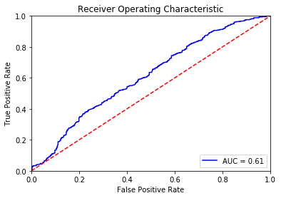
bst = xgb.train(param, dtrain, num_round)Next, we use the trained model to generate predictions for the test dataset and to calculate and plot the AUC:
preds = bst.predict(dtest)
roc_auc_score(y_test, preds)
> 0.609441068887402
The following plot shows our results.
We can also examine the leading predictors by importance of a pull request event’s state:
xgb.plot_importance(bst, importance_type='weight')The following plot shows our results.
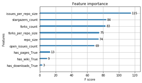
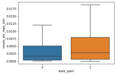
A predictor has different definitions of importance. For this post, we use weight, which is the number of times a predictor appears in the XGBoost trees. The top predictor is the number of open issues normalized by the repository size. Using a box plot, we compare the spread of values for this predictor between closed and still-open pull requests.
After we examine the results and are satisfied with the model performance, we can write predictions back into Amazon DocumentDB.
Storing prediction results
The final step is to store the model predictions back into Amazon DocumentDB. First, we create a new Amazon DocumentDB collection to hold our results, called predictions:
predictions = db['predictions']Then we change the generated predictions to type float, to be accepted by Amazon DocumentDB:
preds = preds.astype(float)We need to associate these predictions with their respective pull request events. Therefore, we use the pull request URL as each document’s ID. We match each prediction to its respective pull request URL and consolidate them in a list:
urls = y_test.index

def gen_preds(url, pred):
    """
    Generate document with prediction of whether pull request will close in 24 hours.
    ID is pull request URL.
    """
    doc = {
        "_id": url,
        "close_24hr_prediction": pred}

    return doc

documents = [gen_preds(url, pred) for url, pred in zip(urls, preds)]
Finally, we use the insert_many command to write the documents to Amazon DocumentDB:
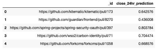
predictions.insert_many(documents, ordered=False)We can query a sample of five documents in the predictions collections to verify that the results have been inserted correctly:
pd.DataFrame(predictions.find({}).limit(5))The following screenshot shows our results.
Cleaning up resources
To save cost, delete the CloudFormation stack you created. This removes all the resources you provisioned using the CloudFormation template, including the VPC, Amazon DocumentDB cluster, and SageMaker instance. For instructions, see Deleting a stack on the AWS CloudFormation console.
Summary
We used SageMaker to analyze data stored in Amazon DocumentDB, conduct descriptive analysis, and build a simple ML model to make predictions, before writing prediction results back into the database.
Amazon DocumentDB provides you with a number of capabilities that help you back up and restore your data based on your use case. For more information, see Best Practices for Amazon DocumentDB. If you’re new to Amazon DocumentDB, see Getting Started with Amazon DocumentDB. If you’re planning to migrate to Amazon DocumentDB, see Migrating to Amazon DocumentDB.
About the Authors
 Annalyn Ng is a Senior Data Scientist with AWS Professional Services, where she develops and deploys machine learning solutions for customers. Annalyn graduated with an MPhil from the University of Cambridge, and blogs about machine learning at algobeans.com. Her book, ’Numsense! Data Science for the Layman’, has been translated into over five languages and is used in top universities as reference text.
 Brian Hess is a Senior Solution Architect Specialist for Amazon DocumentDB (with MongoDB compatibility) at AWS. He has been in the data and analytics space for over 20 years and has extensive experience with relational and NoSQL databases.

How to Avoid Speed Bumps and Stay in the AI Fast Lane with Hybrid Cloud Infrastructure
Cloud or on premises? That’s the question many organizations ask when building AI infrastructure.
Cloud computing can help developers get a fast start with minimal cost. It’s great for early experimentation and supporting temporary needs.
As businesses iterate on their AI models, however, they can become increasingly complex, consume more compute cycles and involve exponentially larger datasets. The costs of data gravity can escalate, with more time and money spent pushing large datasets from where they’re generated to where compute resources reside.
This AI development “speed bump” is often an inflection point where organizations realize there are opex benefits with on-premises or collocated infrastructure. Its fixed costs can support rapid iteration at the lowest “cost per training run,” complementing their cloud usage.
Conversely, for organizations whose datasets are created in the cloud and live there, procuring compute resources adjacent to that data makes sense. Whether on-prem or in the cloud, minimizing data travel — by keeping large volumes as close to compute resources as possible — helps minimize the impact of data gravity on operating costs.
‘Own the Base, Rent the Spike’
Businesses that ultimately embrace hybrid cloud infrastructure trace a familiar trajectory.
One customer developing an image recognition application immediately benefited from a fast, effortless start in the cloud.
As their database grew to millions of images, costs rose and processing slowed, causing their data scientists to become more cautious in refining their models.
At this tipping point — when a fixed cost infrastructure was justified — they shifted training workloads to an on-prem NVIDIA DGX system. This enabled an immediate return to rapid, creative experimentation, allowing the business to build on the great start enabled by the cloud.
The saying “own the base, rent the spike” captures this situation. Enterprise IT provisions on-prem DGX infrastructure to support the steady-state volume of AI workloads and retains the ability to burst to the cloud whenever extra capacity is needed.
It’s this hybrid cloud approach that can secure the continuous availability of compute resources for developers while ensuring the lowest cost per training run.
Delivering the AI Hybrid Cloud with DGX and Google Cloud’s Anthos on Bare Metal
To help businesses embrace hybrid cloud infrastructure, NVIDIA has introduced support for Google Cloud’s Anthos on bare metal for its DGX A100 systems.
For customers using Kubernetes to straddle cloud GPU compute instances and on-prem DGX infrastructure, Anthos on bare metal enables a consistent development and operational experience across deployments, while reducing expensive overhead and improving developer productivity.
This presents several benefits to enterprises. While many have implemented GPU-accelerated AI in their data centers, much of the world retains some legacy x86 compute infrastructure. With Anthos on bare metal, IT can easily add on-prem DGX systems to their infrastructure to tackle AI workloads and manage it the same familiar way, all without the need for a hypervisor layer.
Without the need for a virtual machine, Anthos on bare metal — now generally available — manages application deployment and health across existing environments for more efficient operations. Anthos on bare metal can also manage application containers on a wide variety of performance, GPU-optimized hardware types and allows for direct application access to hardware.
“Anthos on bare metal provides customers with more choice over how and where they run applications and workloads,” said Rayn Veerubhotla, Director of Partner Engineering at Google Cloud. “NVIDIA’s support for Anthos on bare metal means customers can seamlessly deploy NVIDIA’s GPU Device Plugin directly on their hardware, enabling increased performance and flexibility to balance ML workloads across hybrid environments.”
Additionally, teams can access their favorite NVIDIA NGC containers, Helm charts and AI models from anywhere.
With this combination, enterprises can enjoy the rapid start and elasticity of resources offered on Google Cloud, as well as the secure performance of dedicated on-prem DGX infrastructure.
Learn more about Google Cloud’s Anthos.
Learn more about NVIDIA DGX A100.
The post How to Avoid Speed Bumps and Stay in the AI Fast Lane with Hybrid Cloud Infrastructure appeared first on The Official NVIDIA Blog.
Amazon Research Award recipient develops new tool to diagnose dystonia
Dr. Kristina Simonyan and her team created an AI-based deep learning platform that offers patients some peace of mind.Read More
MONAI Imaging Framework Fast-Tracked to Production to Accelerate AI in Healthcare
MONAI — the Medical Open Network for AI, a domain-optimized, open-source framework for healthcare — is now ready for production with the upcoming release of the NVIDIA Clara application framework for AI-powered healthcare and life sciences.
Introduced in April and already adopted by leading healthcare research institutions, MONAI is a PyTorch-based framework that enables the development of AI for medical imaging with industry-specific data handling, high-performance training workflows and reproducible reference implementations of state-of-the-art approaches.
As part of the updated Clara offering, MONAI will come with over 20 pre-trained models, including ones recently developed for COVID-19, as well as the latest training optimizations on NVIDIA DGX A100 GPUs that provide up to a sixfold acceleration in training turnaround time.
“MONAI is becoming the PyTorch of healthcare, paving the way for closer collaboration between data scientists and clinicians,” said Dr. Jayashree Kalpathy-Cramer, director of the QTIM lab at the Athinoula A. Martinos Center for Biomedical Imaging at MGH. “Global adoption of MONAI is fostering collaboration across the globe facilitated by federated learning.”
Adoption by the healthcare ecosystem of MONAI has been tremendous. DKFZ, King’s College London, Mass General, Stanford and Vanderbilt are among those to adopt the AI framework for imaging. MONAI is being used in everything from industry-leading imaging competitions to the first boot camp focused on the framework, held in September, which drew over 550 registrants from 40 countries, including undergraduate university students.
“MONAI is quickly becoming the go-to deep learning framework for healthcare. Getting from research to production is critical for the integration of AI applications into clinical care,” said Dr. Bennett Landman of Vanderbilt University. “NVIDIA’s commitment to community-driven science and allowing the academic community to contribute to a framework that is production-ready will allow for further innovation to build enterprise-ready features.”
New Features
NVIDIA Clara brings the latest breakthroughs in AI-assisted annotation, federated learning and production deployment to the MONAI community.
The latest version introduces a game-changer to AI-assisted annotation that allows radiologists to label complex 3D CT data in one-tenth of the clicks with a new model called DeepGrow 3D. Instead of the traditional time-consuming method of segmenting an organ or lesion image by image or slice by slice, which can be up to 250 clicks for a large organ like the liver, users can segment with far fewer clicks.
Integrated with Fovia Ai’s F.A.S.T. AI Annotation software, NVIDIA Clara’s AI-assisted annotation tools and the new DeepGrow 3D feature can be used for labeling training data as well as assisting radiologists when reading. Fovia offers the XStream HDVR SDK suite to review DICOM images that’s integrated into industry-leading PACS viewers.
AI-assisted annotation is the key to unlocking rich radiology datasets and was recently used to label the public COVID-19 CT dataset published by The Cancer Imaging Archive at the U.S. National Institutes of Health. This labeled dataset was then used in the MICCAI-endorsed COVID-19 Lung CT Lesion Segmentation Challenge.
Clara Federated Learning made possible the recent research collaboration of 20 hospitals around the world to develop a generalized AI model for COVID-19 patients. The EXAM model predicts oxygen requirements in COVID-19 patients, is available on the NGC software registry, and is being evaluated for clinical validation at Mount Sinai Health System in New York, Diagnósticos da America SA in Brazil, NIHR Cambridge Biomedical Research Centre in the U.K. and the NIH.
“The MONAI software framework provides key components for training and evaluating imaging-based deep learning models, and its open-source approach is fostering a growing community that is contributing exciting advances, such as federated learning,” said Dr. Daniel Rubin, professor of biomedical data science, radiology and medicine at Stanford University.
NVIDIA is additionally expanding its release of NVIDIA Clara to digital pathology applications, where the sheer sizes of images would choke off-the-shelf open-source AI tools. Clara for pathology early access contains reference pipelines for both training and deployment of AI applications.
“Healthcare data interoperability, model deployment and clinical pathway integration are an increasingly complex and intertwined topic, with significant field-specific expertise,” said Jorge Cardoso, CTO of the London Medical Imaging and AI Centre for Value-based Healthcare. “Project MONAI, jointly with the rest of the NVIDIA Clara ecosystem, will help deliver improvements to patient care and optimize hospital operations.”
Learn more about NVIDIA Clara Train 4.0 and subscribe to NVIDIA healthcare news.
The post MONAI Imaging Framework Fast-Tracked to Production to Accelerate AI in Healthcare appeared first on The Official NVIDIA Blog.

NVIDIA Launches Inception Alliance with GE Healthcare and Nuance to Accelerate Medical Imaging AI Startups
Just over 125 years ago, on Nov. 8, 1895, the world’s first X-ray image was captured. It was a breakthrough that set the stage for the modern medical imaging industry.
Over the decades, an entire ecosystem of medical imaging hardware and software came to be, with AI startups now playing a key role within it.
Today we’re announcing the NVIDIA Inception Alliance for Healthcare, an initiative where medical AI startups have new opportunities to chart innovations and accelerate their success with the help of NVIDIA and its healthcare industry partners.
Premier members of NVIDIA Inception, our accelerator program for 6,500+ startups across 90 countries in AI and data sciences, can now join the GE Healthcare Edison Developer Program. Through integration with the GE Healthcare Edison Platform, these startups gain access to GE Healthcare’s global network to scale clinical and commercial activities within their expansive install base of 4 million imaging, mobile diagnostics and monitoring units across 160 countries with 230 million exams and associated data.
Premier members with FDA clearance also can join the Nuance AI Marketplace for Diagnostic Imaging. The Nuance AI Marketplace brings AI into the radiology workflow by connecting developers directly with radiology subscribers. It offers AI developers a single API to connect their AI solutions to radiologists across 8,000 healthcare facilities that use the Nuance PowerShare Network. And it gives radiology subscribers a one-stop shop to review, try, validate and buy AI models — bridging the technology divide to make AI useful, usable and used.
A Prescription for Growth
NVIDIA Inception, which recently added its 1,000th healthcare AI startup, offers its members a variety of ongoing benefits, including go-to-market support, technology assistance and access to NVIDIA expertise — all tailored to a business’s maturity stage. Startups get access to training through the NVIDIA Deep Learning Institute, preferred pricing on hardware through our global network of distributors, invitations to exclusive networking events and more.
To nurture the growth of AI startups in healthcare, and ultimately the entire medical ecosystem, NVIDIA is working with healthcare giants to offer Inception members an accelerated go-to-market path.
The NVIDIA Inception Alliance for Healthcare will forge new ways to grow through targeted networking, AI training, early access to technology, pitch competitions and technology integration. Members will receive customized training and support to develop, deploy and integrate NVIDIA GPU-accelerated apps everywhere within the medical imaging ecosystem.
Select startup members will have direct access to engage joint customers, in addition to marketing promotion of their results. The initiative will kick off with a pitch competition for leading AI startups in medical imaging and related supporting fields.
“Startups are on the forefront of innovation and the GE Healthcare Edison Developer Program provides them access to the world’s largest installed base of medical devices and customers,” said Karley Yoder, vice president and general manager of Artificial Intelligence at GE Healthcare. “Bringing together the world-class capabilities from industry-leading partners creates a fast-track to accelerate innovation in a connected ecosystem that will help improve the quality of care, lower healthcare costs and deliver better outcomes for patients.”
“With Nuance’s deep understanding of radiologists’ needs and workflow, we are uniquely positioned to help them transform healthcare by harnessing AI. The Nuance AI Marketplace gives radiologists the ability to easily purchase, validate and use AI models within solutions they use every day, so they can work smarter and more efficiently,” said Karen Holzberger, senior vice president and general manager of the Diagnostic Division at Nuance. “The AI models help radiologists focus their time and expertise on the right case at the right time, alleviate many repetitive, mundane tasks and, ultimately, improve patient care — and save more lives. Connecting NVIDIA Inception startup members to the Nuance AI Marketplace is a natural fit — and creates a connection for startups that benefits the entire industry.”
Learn more at the NVIDIA RSNA 2020 Special Address, which is open to the public on Tuesday, Dec. 1, at 6 p.m. CT. Kimberly Powell, NVIDIA’s vice president of healthcare, will discuss how we’re working with medical imaging companies, radiologists, data scientists, researchers and medical device companies to bring workflow acceleration, AI models and deployment platforms to the medical imaging ecosystem.
Subscribe to NVIDIA healthcare news.
The post NVIDIA Launches Inception Alliance with GE Healthcare and Nuance to Accelerate Medical Imaging AI Startups appeared first on The Official NVIDIA Blog.