The confusion matrix, a ubiquitous visualization for helping people evaluate machine learning models, is a tabular layout that compares predicted class labels against actual class labels over all data instances. We conduct formative research with machine learning practitioners at Apple and find that conventional confusion matrices do not support more complex data-structures found in modern-day applications, such as hierarchical and multi-output labels. To express such variations of confusion matrices, we design an algebra that models confusion matrices as probability distributions. Based on…Apple Machine Learning Research
Federated Learning with Formal Differential Privacy Guarantees
In 2017, Google introduced federated learning (FL), an approach that enables mobile devices to collaboratively train machine learning (ML) models while keeping the raw training data on each user’s device, decoupling the ability to do ML from the need to store the data in the cloud. Since its introduction, Google has continued to actively engage in FL research and deployed FL to power many features in Gboard, including next word prediction, emoji suggestion and out-of-vocabulary word discovery. Federated learning is improving the “Hey Google” detection models in Assistant, suggesting replies in Google Messages, predicting text selections, and more.
While FL allows ML without raw data collection, differential privacy (DP) provides a quantifiable measure of data anonymization, and when applied to ML can address concerns about models memorizing sensitive user data. This too has been a top research priority, and has yielded one of the first production uses of DP for analytics with RAPPOR in 2014, our open-source DP library, Pipeline DP, and TensorFlow Privacy.
Through a multi-year, multi-team effort spanning fundamental research and product integration, today we are excited to announce that we have deployed a production ML model using federated learning with a rigorous differential privacy guarantee. For this proof-of-concept deployment, we utilized the DP-FTRL algorithm to train a recurrent neural network to power next-word-prediction for Spanish-language Gboard users. To our knowledge, this is the first production neural network trained directly on user data announced with a formal DP guarantee (technically ρ=0.81 zero-Concentrated-Differential-Privacy, zCDP, discussed in detail below). Further, the federated approach offers complimentary data minimization advantages, and the DP guarantee protects all of the data on each device, not just individual training examples.
Data Minimization and Anonymization in Federated Learning
Along with fundamentals like transparency and consent, the privacy principles of data minimization and anonymization are important in ML applications that involve sensitive data.
Federated learning systems structurally incorporate the principle of data minimization. FL only transmits minimal updates for a specific model training task (focused collection), limits access to data at all stages, processes individuals’ data as early as possible (early aggregation), and discards both collected and processed data as soon as possible (minimal retention).
Another principle that is important for models trained on user data is anonymization, meaning that the final model should not memorize information unique to a particular individual’s data, e.g., phone numbers, addresses, credit card numbers. However, FL on its own does not directly tackle this problem.
The mathematical concept of DP allows one to formally quantify this principle of anonymization. Differentially private training algorithms add random noise during training to produce a probability distribution over output models, and ensure that this distribution doesn’t change too much given a small change to the training data; ρ-zCDP quantifies how much the distribution could possibly change. We call this example-level DP when adding or removing a single training example changes the output distribution on models in a provably minimal way.
Showing that deep learning with example-level differential privacy was even possible in the simpler setting of centralized training was a major step forward in 2016. Achieved by the DP-SGD algorithm, the key was amplifying the privacy guarantee by leveraging the randomness in sampling training examples (“amplification-via-sampling”).
However, when users can contribute multiple examples to the training dataset, example-level DP is not necessarily strong enough to ensure the users’ data isn’t memorized. Instead, we have designed algorithms for user-level DP, which requires that the output distribution of models doesn’t change even if we add/remove all of the training examples from any one user (or all the examples from any one device in our application). Fortunately, because FL summarizes all of a user’s training data as a single model update, federated algorithms are well-suited to offering user-level DP guarantees.
Both limiting the contributions from one user and adding noise can come at the expense of model accuracy, however, so maintaining model quality while also providing strong DP guarantees is a key research focus.
The Challenging Path to Federated Learning with Differential Privacy
In 2018, we introduced the DP-FedAvg algorithm, which extended the DP-SGD approach to the federated setting with user-level DP guarantees, and in 2020 we deployed this algorithm to mobile devices for the first time. This approach ensures the training mechanism is not too sensitive to any one user’s data, and empirical privacy auditing techniques rule out some forms of memorization.
However, the amplification-via-samping argument is essential to providing a strong DP guarantee for DP-FedAvg, but in a real-world cross-device FL system ensuring devices are subsampled precisely and uniformly at random from a large population would be complex and hard to verify. One challenge is that devices choose when to connect (or “check in”) based on many external factors (e.g., requiring the device is idle, on unmetered WiFi, and charging), and the number of available devices can vary substantially.
Achieving a formal privacy guarantee requires a protocol that does all of the following:
- Makes progress on training even as the set of devices available varies significantly with time.
- Maintains privacy guarantees even in the face of unexpected or arbitrary changes in device availability.
- For efficiency, allows client devices to locally decide whether they will check in to the server in order to participate in training, independent of other devices.
Initial work on privacy amplification via random check-ins highlighted these challenges and introduced a feasible protocol, but it would have required complex changes to our production infrastructure to deploy. Further, as with the amplification-via-sampling analysis of DP-SGD, the privacy amplification possible with random check-ins depends on a large number of devices being available. For example, if only 1000 devices are available for training, and participation of at least 1000 devices is needed in each training step, that requires either 1) including all devices currently available and paying a large privacy cost since there is no randomness in the selection, or 2) pausing the protocol and not making progress until more devices are available.
Achieving Provable Differential Privacy for Federated Learning with DP-FTRL
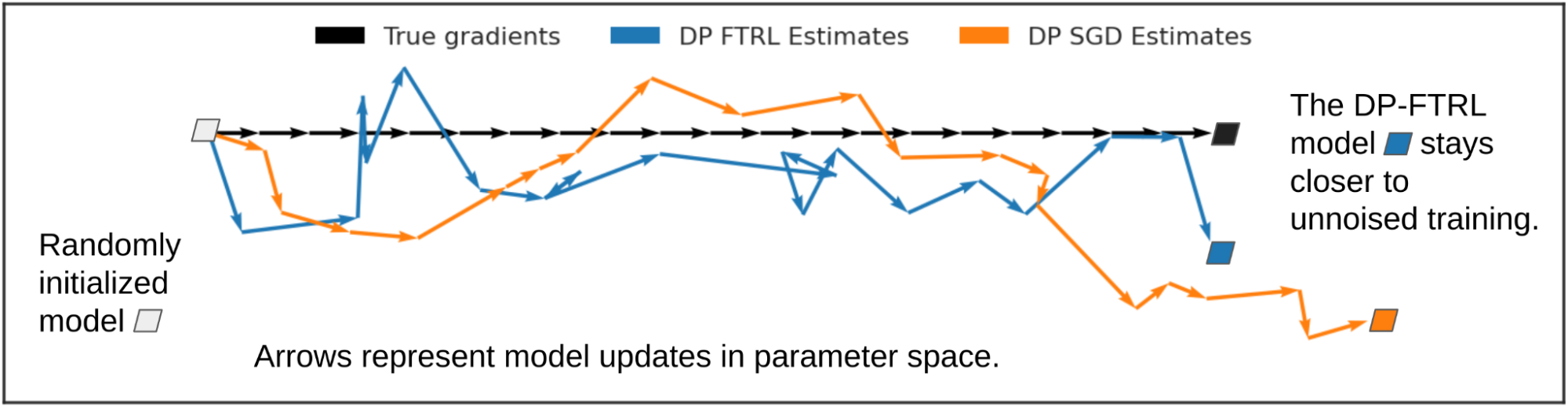
To address this challenge, the DP-FTRL algorithm is built on two key observations: 1) the convergence of gradient-descent-style algorithms depends primarily not on the accuracy of individual gradients, but the accuracy of cumulative sums of gradients; and 2) we can provide accurate estimates of cumulative sums with a strong DP guarantee by utilizing negatively correlated noise, added by the aggregating server: essentially, adding noise to one gradient and subtracting that same noise from a later gradient. DP-FTRL accomplishes this efficiently using the Tree Aggregation algorithm [1, 2].
The graphic below illustrates how estimating cumulative sums rather than individual gradients can help. We look at how the noise introduced by DP-FTRL and DP-SGD influence model training, compared to the true gradients (without added noise; in black) which step one unit to the right on each iteration. The individual DP-FTRL gradient estimates (blue), based on cumulative sums, have larger mean-squared-error than the individually-noised DP-SGD estimates (orange), but because the DP-FTRL noise is negatively correlated, some of it cancels out from step to step, and the overall learning trajectory stays closer to the true gradient descent steps.
|
To provide a strong privacy guarantee, we limit the number of times a user contributes an update. Fortunately, sampling-without-replacement is relatively easy to implement in production FL infrastructure: each device can remember locally which models it has contributed to in the past, and choose to not connect to the server for any later rounds for those models.
Production Training Details and Formal DP Statements
For the production DP-FTRL deployment introduced above, each eligible device maintains a local training cache consisting of user keyboard input, and when participating computes an update to the model which makes it more likely to suggest the next word the user actually typed, based on what has been typed so far. We ran DP-FTRL on this data to train a recurrent neural network with ~1.3M parameters. Training ran for 2000 rounds over six days, with 6500 devices participating per round. To allow for the DP guarantee, devices participated in training at most once every 24 hours. Model quality improved over the previous DP-FedAvg trained model, which offered empirically-tested privacy advantages over non-DP models, but lacked a meaningful formal DP guarantee.
The training mechanism we used is available in open-source in TensorFlow Federated and TensorFlow Privacy, and with the parameters used in our production deployment it provides a meaningfully strong privacy guarantee. Our analysis gives ρ=0.81 zCDP at the user level (treating all the data on each device as a different user), where smaller numbers correspond to better privacy in a mathematically precise way. As a comparison, this is stronger than the ρ=2.63 zCDP guarantee chosen by the 2020 US Census.
Next Steps
While we have reached the milestone of deploying a production FL model using a mechanism that provides a meaningfully small zCDP, our research journey continues. We are still far from being able to say this approach is possible (let alone practical) for most ML models or product applications, and other approaches to private ML exist. For example, membership inference tests and other empirical privacy auditing techniques can provide complimentary safeguards against leakage of users’ data. Most importantly, we see training models with user-level DP with even a very large zCDP as a substantial step forward, because it requires training with a DP mechanism that bounds the sensitivity of the model to any one user’s data. Further, it smooths the road to later training models with improved privacy guarantees as better algorithms or more data become available. We are excited to continue the journey toward maximizing the value that ML can deliver while minimizing potential privacy costs to those who contribute training data.
Acknowledgements
The authors would like to thank Alex Ingerman and Om Thakkar for significant impact on the blog post itself, as well as the teams at Google that helped develop these ideas and bring them to practice:
- Core research team: Galen Andrew, Borja Balle, Peter Kairouz, Daniel Ramage, Shuang Song, Thomas Steinke, Andreas Terzis, Om Thakkar, Zheng Xu
- FL infrastructure team: Katharine Daly, Stefan Dierauf, Hubert Eichner, Igor Pisarev, Timon Van Overveldt, Chunxiang Zheng
- Gboard team: Angana Ghosh, Xu Liu, Yuanbo Zhang
- Speech team: Françoise Beaufays, Mingqing Chen, Rajiv Mathews, Vidush Mukund, Igor Pisarev, Swaroop Ramaswamy, Dan Zivkovic

Constrained Reweighting for Training Deep Neural Nets with Noisy Labels
Over the past several years, deep neural networks (DNNs) have been quite successful in driving impressive performance gains in several real-world applications, from image recognition to genomics. However, modern DNNs often have far more trainable model parameters than the number of training examples and the resulting overparameterized networks can easily overfit to noisy or corrupted labels (i.e., examples that are assigned a wrong class label). As a consequence, training with noisy labels often leads to degradation in accuracy of the trained model on clean test data. Unfortunately, noisy labels can appear in several real-world scenarios due to multiple factors, such as errors and inconsistencies in manual annotation and the use of inherently noisy label sources (e.g., the internet or automated labels from an existing system).
Earlier work has shown that representations learned by pre-training large models with noisy data can be useful for prediction when used in a linear classifier trained with clean data. In principle, it is possible to directly train machine learning (ML) models on noisy data without resorting to this two-stage approach. To be successful, such alternative methods should have the following properties: (i) they should fit easily into standard training pipelines with little computational or memory overhead; (ii) they should be applicable in “streaming” settings where new data is continuously added during training; and (iii) they should not require data with clean labels.
In “Constrained Instance and Class Reweighting for Robust Learning under Label Noise”, we propose a novel and principled method, named Constrained Instance reWeighting (CIW), with these properties that works by dynamically assigning importance weights both to individual instances and to class labels in a mini-batch, with the goal of reducing the effect of potentially noisy examples. We formulate a family of constrained optimization problems that yield simple solutions for these importance weights. These optimization problems are solved per mini-batch, which avoids the need to store and update the importance weights over the full dataset. This optimization framework also provides a theoretical perspective for existing label smoothing heuristics that address label noise, such as label bootstrapping. We evaluate the method with varying amounts of synthetic noise on the standard CIFAR-10 and CIFAR-100 benchmarks and observe considerable performance gains over several existing methods.
Method
Training ML models involves minimizing a loss function that indicates how well the current parameters fit to the given training data. In each training step, this loss is approximately calculated as a (weighted) sum of the losses of individual instances in the mini-batch of data on which it is operating. In standard training, each instance is treated equally for the purpose of updating the model parameters, which corresponds to assigning uniform (i.e., equal) weights across the mini-batch.
However, empirical observations made in earlier works reveal that noisy or mislabeled instances tend to have higher loss values than those that are clean, particularly during early to mid-stages of training. Thus, assigning uniform importance weights to all instances means that due to their higher loss values, the noisy instances can potentially dominate the clean instances and degrade the accuracy on clean test data.
Motivated by these observations, we propose a family of constrained optimization problems that solve this problem by assigning importance weights to individual instances in the dataset to reduce the effect of those that are likely to be noisy. This approach provides control over how much the weights deviate from uniform, as quantified by a divergence measure. It turns out that for several types of divergence measures, one can obtain simple formulae for the instance weights. The final loss is computed as the weighted sum of individual instance losses, which is used for updating the model parameters. We call this the Constrained Instance reWeighting (CIW) method. This method allows for controlling the smoothness or peakiness of the weights through the choice of divergence and a corresponding hyperparameter.
|
| Schematic of the proposed Constrained Instance reWeighting (CIW) method. |
Illustration with Decision Boundary on a 2D Dataset
As an example to illustrate the behavior of this method, we consider a noisy version of the Two Moons dataset, which consists of randomly sampled points from two classes in the shape of two half moons. We corrupt 30% of the labels and train a multilayer perceptron network on it for binary classification. We use the standard binary cross-entropy loss and an SGD with momentum optimizer to train the model. In the figure below (left panel), we show the data points and visualize an acceptable decision boundary separating the two classes with a dotted line. The points marked red in the upper half-moon and those marked green in the lower half-moon indicate noisy data points.
The baseline model trained with the binary cross-entropy loss assigns uniform weights to the instances in each mini-batch, thus eventually overfitting to the noisy instances and resulting in a poor decision boundary (middle panel in the figure below).
The CIW method reweights the instances in each mini-batch based on their corresponding loss values (right panel in the figure below). It assigns larger weights to the clean instances that are located on the correct side of the decision boundary and damps the effect of noisy instances that incur a higher loss value. Smaller weights for noisy instances help in preventing the model from overfitting to them, thus allowing the model trained with CIW to successfully converge to a good decision boundary by avoiding the impact of label noise.
 |
| Illustration of decision boundary as the training proceeds for the baseline and the proposed CIW method on the Two Moons dataset. Left: Noisy dataset with a desirable decision boundary. Middle: Decision boundary for standard training with cross-entropy loss. Right: Training with the CIW method. The size of the dots in (middle) and (right) are proportional to the importance weights assigned to these examples in the minibatch. |
<!–
 |
 |
 |
| Illustration of decision boundary as the training proceeds for the baseline and the proposed CIW method on the Two Moons dataset. Left: Noisy dataset with a desirable decision boundary. Middle: Decision boundary for standard training with cross-entropy loss. Right: Training with the CIW method. The size of the dots in (middle) and (right) are proportional to the importance weights assigned to these examples in the minibatch. |
–>
Constrained Class reWeighting
Instance reweighting assigns lower weights to instances with higher losses. We further extend this intuition to assign importance weights over all possible class labels. Standard training uses a one-hot label vector as the class weights, assigning a weight of 1 to the labeled class and 0 to all other classes. However, for the potentially mislabeled instances, it is reasonable to assign non-zero weights to classes that could be the true label. We obtain these class weights as solutions to a family of constrained optimization problems where the deviation of the class weights from the label one-hot distribution, as measured by a divergence of choice, is controlled by a hyperparameter.
Again, for several divergence measures, we can obtain simple formulae for the class weights. We refer to this as Constrained Instance and Class reWeighting (CICW). The solution to this optimization problem also recovers the earlier proposed methods based on static label bootstrapping (also referred as label smoothing) when the divergence is taken to be total variation distance. This provides a theoretical perspective on the popular method of static label bootstrapping.
Using Instance Weights with Mixup
We also propose a way to use the obtained instance weights with mixup, which is a popular method for regularizing models and improving prediction performance. It works by sampling a pair of examples from the original dataset and generating a new artificial example using a random convex combination of these. The model is trained by minimizing the loss on these mixed-up data points. Vanilla mixup is oblivious to the individual instance losses, which might be problematic for noisy data because mixup will treat clean and noisy examples equally. Since a high instance weight obtained with our CIW method is more likely to indicate a clean example, we use our instance weights to do a biased sampling for mixup and also use the weights in convex combinations (instead of random convex combinations in vanilla mixup). This results in biasing the mixed-up examples towards clean data points, which we refer to as CICW-Mixup.
We apply these methods with varying amounts of synthetic noise (i.e., the label for each instance is randomly flipped to other labels) on the standard CIFAR-10 and CIFAR-100 benchmark datasets. We show the test accuracy on clean data with symmetric synthetic noise where the noise rate is varied between 0.2 and 0.8.
We observe that the proposed CICW outperforms several methods and matches the results of dynamic mixup, which maintains the importance weights over the full training set with mixup. Using our importance weights with mixup in CICW-M, resulted in significantly improved performance vs these methods, particularly for larger noise rates (as shown by lines above and to the right in the graphs below).
 |
| Test accuracy on clean data while varying the amount of symmetric synthetic noise in the training data for CIFAR-10 and CIFAR-100. Methods compared are: standard Cross-Entropy Loss (CE), Bi-tempered Loss, Active-Passive Normalized Loss, the proposed CICW, Mixup, Dynamic Mixup, and the proposed CICW-Mixup. |
Summary and Future Directions
We formulate a novel family of constrained optimization problems for tackling label noise that yield simple mathematical formulae for reweighting the training instances and class labels. These formulations also provide a theoretical perspective on existing label smoothing–based methods for learning with noisy labels. We also propose ways for using the instance weights with mixup that results in further significant performance gains over instance and class reweighting. Our method operates solely at the level of mini-batches, which avoids the extra overhead of maintaining dataset-level weights as in some of the recent methods.
As a direction for future work, we would like to evaluate the method on realistic noisy labels that are encountered in large scale practical settings. We also believe that studying the interaction of our framework with label smoothing is an interesting direction that can result in a loss adaptive version of label smoothing. We are also excited to release the code for CICW, now available on Github.
Acknowledgements
We’d like to thank Kevin Murphy for providing constructive feedback during the course of the project.
Improving question-answering models that use data from tables
Novel pretraining method enables increases of 5% to 14% on five different evaluation metrics.Read More
Using artificial intelligence to find anomalies hiding in massive datasets
Identifying a malfunction in the nation’s power grid can be like trying to find a needle in an enormous haystack. Hundreds of thousands of interrelated sensors spread across the U.S. capture data on electric current, voltage, and other critical information in real time, often taking multiple recordings per second.
Researchers at the MIT-IBM Watson AI Lab have devised a computationally efficient method that can automatically pinpoint anomalies in those data streams in real time. They demonstrated that their artificial intelligence method, which learns to model the interconnectedness of the power grid, is much better at detecting these glitches than some other popular techniques.
Because the machine-learning model they developed does not require annotated data on power grid anomalies for training, it would be easier to apply in real-world situations where high-quality, labeled datasets are often hard to come by. The model is also flexible and can be applied to other situations where a vast number of interconnected sensors collect and report data, like traffic monitoring systems. It could, for example, identify traffic bottlenecks or reveal how traffic jams cascade.
“In the case of a power grid, people have tried to capture the data using statistics and then define detection rules with domain knowledge to say that, for example, if the voltage surges by a certain percentage, then the grid operator should be alerted. Such rule-based systems, even empowered by statistical data analysis, require a lot of labor and expertise. We show that we can automate this process and also learn patterns from the data using advanced machine-learning techniques,” says senior author Jie Chen, a research staff member and manager of the MIT-IBM Watson AI Lab.
The co-author is Enyan Dai, an MIT-IBM Watson AI Lab intern and graduate student at the Pennsylvania State University. This research will be presented at the International Conference on Learning Representations.
Probing probabilities
The researchers began by defining an anomaly as an event that has a low probability of occurring, like a sudden spike in voltage. They treat the power grid data as a probability distribution, so if they can estimate the probability densities, they can identify the low-density values in the dataset. Those data points which are least likely to occur correspond to anomalies.
Estimating those probabilities is no easy task, especially since each sample captures multiple time series, and each time series is a set of multidimensional data points recorded over time. Plus, the sensors that capture all that data are conditional on one another, meaning they are connected in a certain configuration and one sensor can sometimes impact others.
To learn the complex conditional probability distribution of the data, the researchers used a special type of deep-learning model called a normalizing flow, which is particularly effective at estimating the probability density of a sample.
They augmented that normalizing flow model using a type of graph, known as a Bayesian network, which can learn the complex, causal relationship structure between different sensors. This graph structure enables the researchers to see patterns in the data and estimate anomalies more accurately, Chen explains.
“The sensors are interacting with each other, and they have causal relationships and depend on each other. So, we have to be able to inject this dependency information into the way that we compute the probabilities,” he says.
This Bayesian network factorizes, or breaks down, the joint probability of the multiple time series data into less complex, conditional probabilities that are much easier to parameterize, learn, and evaluate. This allows the researchers to estimate the likelihood of observing certain sensor readings, and to identify those readings that have a low probability of occurring, meaning they are anomalies.
Their method is especially powerful because this complex graph structure does not need to be defined in advance — the model can learn the graph on its own, in an unsupervised manner.
A powerful technique
They tested this framework by seeing how well it could identify anomalies in power grid data, traffic data, and water system data. The datasets they used for testing contained anomalies that had been identified by humans, so the researchers were able to compare the anomalies their model identified with real glitches in each system.
Their model outperformed all the baselines by detecting a higher percentage of true anomalies in each dataset.
“For the baselines, a lot of them don’t incorporate graph structure. That perfectly corroborates our hypothesis. Figuring out the dependency relationships between the different nodes in the graph is definitely helping us,” Chen says.
Their methodology is also flexible. Armed with a large, unlabeled dataset, they can tune the model to make effective anomaly predictions in other situations, like traffic patterns.
Once the model is deployed, it would continue to learn from a steady stream of new sensor data, adapting to possible drift of the data distribution and maintaining accuracy over time, says Chen.
Though this particular project is close to its end, he looks forward to applying the lessons he learned to other areas of deep-learning research, particularly on graphs.
Chen and his colleagues could use this approach to develop models that map other complex, conditional relationships. They also want to explore how they can efficiently learn these models when the graphs become enormous, perhaps with millions or billions of interconnected nodes. And rather than finding anomalies, they could also use this approach to improve the accuracy of forecasts based on datasets or streamline other classification techniques.
This work was funded by the MIT-IBM Watson AI Lab and the U.S. Department of Energy.
Deep-learning technique predicts clinical treatment outcomes
When it comes to treatment strategies for critically ill patients, clinicians want to be able to consider all their options and timing of administration, and make the optimal decision for their patients. While clinician experience and study has helped them to be successful in this effort, not all patients are the same, and treatment decisions at this crucial time could mean the difference between patient improvement and quick deterioration. Therefore, it would be helpful for doctors to be able to take a patient’s previous known health status and received treatments and use that to predict that patient’s health outcome under different treatment scenarios, in order to pick the best path.
Now, a deep-learning technique, called G-Net, from researchers at MIT and IBM provides a window into causal counterfactual prediction, affording physicians the opportunity to explore how a patient might fare under different treatment plans. The foundation of G-Net is the g-computation algorithm, a causal inference method that estimates the effect of dynamic exposures in the presence of measured confounding variables — ones that may influence both treatments and outcomes. Unlike previous implementations of the g-computation framework, which have used linear modeling approaches, G-Net uses recurrent neural networks (RNN), which have node connections that allow them to better model temporal sequences with complex and nonlinear dynamics, like those found in the physiological and clinical time series data. In this way, physicians can develop alternative plans based on patient history and test them before making a decision.
“Our ultimate goal is to develop a machine learning technique that would allow doctors to explore various ‘What if’ scenarios and treatment options,” says Li-wei Lehman, MIT research scientist in the MIT Institute for Medical Engineering and Science and an MIT-IBM Watson AI Lab project lead. “A lot of work has been done in terms of deep learning for counterfactual prediction but [it’s] been focusing on a point exposure setting,” or a static, time-varying treatment strategy, which doesn’t allow for adjustment of treatments as patient history changes. However, her team’s new prediction approach provides for treatment plan flexibility and chances for treatment alteration over time as patient covariate history and past treatments change. “G-Net is the first deep-learning approach based on g-computation that can predict both the population-level and individual-level treatment effects under dynamic and time varying treatment strategies.”
The research, which was recently published in the Proceedings of Machine Learning Research, was co-authored by Rui Li MEng ’20, Stephanie Hu MEng ’21, former MIT postdoc Mingyu Lu MD, graduate student Yuria Utsumi, IBM research staff member Prithwish Chakraborty, IBM Research director of Hybrid Cloud Services Daby Sow, IBM data scientist Piyush Madan, IBM research scientist Mohamed Ghalwash, and IBM research scientist Zach Shahn.
Tracking disease progression
To build, validate, and test G-Net’s predictive abilities, the researchers considered the circulatory system in septic patients in the ICU. During critical care, doctors need to make trade-offs and judgement calls, such as ensuring the organs are receiving adequate blood supply without overworking the heart. For this, they could give intravenous fluids to patients to increase blood pressure; however, too much can cause edema. Alternatively, physicians can administer vasopressors, which act to contract blood vessels and raise blood pressure.
In order to mimic this and demonstrate G-Net’s proof-of-concept, the team used CVSim, a mechanistic model of a human cardiovascular system that’s governed by 28 input variables characterizing the system’s current state, such as arterial pressure, central venous pressure, total blood volume, and total peripheral resistance, and modified it to simulate various disease processes (e.g., sepsis or blood loss) and effects of interventions (e.g., fluids and vasopressors). The researchers used CVSim to generate observational patient data for training and for “ground truth” comparison against counterfactual prediction. In their G-Net architecture, the researchers ran two RNNs to handle and predict variables that are continuous, meaning they can take on a range of values, like blood pressure, and categorical variables, which have discrete values, like the presence or absence of pulmonary edema. The researchers simulated the health trajectories of thousands of “patients” exhibiting symptoms under one treatment regime, let’s say A, for 66 timesteps, and used them to train and validate their model.
Testing G-Net’s prediction capability, the team generated two counterfactual datasets. Each contained roughly 1,000 known patient health trajectories, which were created from CVSim using the same “patient” condition as the starting point under treatment A. Then at timestep 33, treatment changed to plan B or C, depending on the dataset. The team then performed 100 prediction trajectories for each of these 1,000 patients, whose treatment and medical history was known up until timestep 33 when a new treatment was administered. In these cases, the prediction agreed well with the “ground-truth” observations for individual patients and averaged population-level trajectories.
A cut above the rest
Since the g-computation framework is flexible, the researchers wanted to examine G-Net’s prediction using different nonlinear models — in this case, long short-term memory (LSTM) models, which are a type of RNN that can learn from previous data patterns or sequences — against the more classical linear models and a multilayer perception model (MLP), a type of neural network that can make predictions using a nonlinear approach. Following a similar setup as before, the team found that the error between the known and predicted cases was smallest in the LSTM models compared to the others. Since G-Net is able to model the temporal patterns of the patient’s ICU history and past treatment, whereas a linear model and MLP cannot, it was better able to predict the patient’s outcome.
The team also compared G-Net’s prediction in a static, time-varying treatment setting against two state-of-the-art deep-learning based counterfactual prediction approaches, a recurrent marginal structural network (rMSN) and a counterfactual recurrent neural network (CRN), as well as a linear model and an MLP. For this, they investigated a model for tumor growth under no treatment, radiation, chemotherapy, and both radiation and chemotherapy scenarios. “Imagine a scenario where there’s a patient with cancer, and an example of a static regime would be if you only give a fixed dosage of chemotherapy, radiation, or any kind of drug, and wait until the end of your trajectory,” comments Lu. For these investigations, the researchers generated simulated observational data using tumor volume as the primary influence dictating treatment plans and demonstrated that G-Net outperformed the other models. One potential reason could be because g-computation is known to be more statistically efficient than rMSN and CRN, when models are correctly specified.
While G-Net has done well with simulated data, more needs to be done before it can be applied to real patients. Since neural networks can be thought of as “black boxes” for prediction results, the researchers are beginning to investigate the uncertainty in the model to help ensure safety. In contrast to these approaches that recommend an “optimal” treatment plan without any clinician involvement, “as a decision support tool, I believe that G-Net would be more interpretable, since the clinicians would input treatment strategies themselves,” says Lehman, and “G-Net will allow them to be able to explore different hypotheses.” Further, the team has moved on to using real data from ICU patients with sepsis, bringing it one step closer to implementation in hospitals.
“I think it is pretty important and exciting for real-world applications,” says Hu. “It’d be helpful to have some way to predict whether or not a treatment might work or what the effects might be — a quicker iteration process for developing these hypotheses for what to try, before actually trying to implement them in in a years-long, potentially very involved and very invasive type of clinical trial.”
This research was funded by the MIT-IBM Watson AI Lab.
More sensitive X-ray imaging
Scintillators are materials that emit light when bombarded with high-energy particles or X-rays. In medical or dental X-ray systems, they convert incoming X-ray radiation into visible light that can then be captured using film or photosensors. They’re also used for night-vision systems and for research, such as in particle detectors or electron microscopes.
Researchers at MIT have now shown how one could improve the efficiency of scintillators by at least tenfold, and perhaps even a hundredfold, by changing the material’s surface to create certain nanoscale configurations, such as arrays of wave-like ridges. While past attempts to develop more efficient scintillators have focused on finding new materials, the new approach could in principle work with any of the existing materials.
Though it will require more time and effort to integrate their scintillators into existing X-ray machines, the team believes that this method might lead to improvements in medical diagnostic X-rays or CT scans, to reduce dose exposure and improve image quality. In other applications, such as X-ray inspection of manufactured parts for quality control, the new scintillators could enable inspections with higher accuracy or at faster speeds.
The findings are described today in the journal Science, in a paper by MIT doctoral students Charles Roques-Carmes and Nicholas Rivera; MIT professors Marin Soljacic, Steven Johnson, and John Joannopoulos; and 10 others.
While scintillators have been in use for some 70 years, much of the research in the field has focused on developing new materials that produce brighter or faster light emissions. The new approach instead applies advances in nanotechnology to existing materials. By creating patterns in scintillator materials at a length scale comparable to the wavelengths of the light being emitted, the team found that it was possible to dramatically change the material’s optical properties.
To make what they coined “nanophotonic scintillators,” Roques-Carmes says, “you can directly make patterns inside the scintillators, or you can glue on another material that would have holes on the nanoscale. The specifics depend on the exact structure and material.” For this research, the team took a scintillator and made holes spaced apart by roughly one optical wavelength, or about 500 nanometers (billionths of a meter).
“The key to what we’re doing is a general theory and framework we have developed,” Rivera says. This allows the researchers to calculate the scintillation levels that would be produced by any arbitrary configuration of nanophotonic structures. The scintillation process itself involves a series of steps, making it complicated to unravel. The framework the team developed involves integrating three different types of physics, Roques-Carmes says. Using this system they have found a good match between their predictions and the results of their subsequent experiments.
The experiments showed a tenfold improvement in emission from the treated scintillator. “So, this is something that might translate into applications for medical imaging, which are optical photon-starved, meaning the conversion of X-rays to optical light limits the image quality. [In medical imaging,] you do not want to irradiate your patients with too much of the X-rays, especially for routine screening, and especially for young patients as well,” Roques-Carmes says.
“We believe that this will open a new field of research in nanophotonics,” he adds. “You can use a lot of the existing work and research that has been done in the field of nanophotonics to improve significantly on existing materials that scintillate.”
“The research presented in this paper is hugely significant,” says Rajiv Gupta, chief of neuroradiology at Massachusetts General Hospital and an associate professor at Harvard Medical School, who was not associated with this work. “Nearly all detectors used in the $100 billion [medical X-ray] industry are indirect detectors,” which is the type of detector the new findings apply to, he says. “Everything that I use in my clinical practice today is based on this principle. This paper improves the efficiency of this process by 10 times. If this claim is even partially true, say the improvement is two times instead of 10 times, it would be transformative for the field!”
Soljacic says that while their experiments proved a tenfold improvement in emission could be achieved in particular systems, by further fine-tuning the design of the nanoscale patterning, “we also show that you can get up to 100 times [improvement] in certain scintillator systems, and we believe we also have a path toward making it even better,” he says.
Soljacic points out that in other areas of nanophotonics, a field that deals with how light interacts with materials that are structured at the nanometer scale, the development of computational simulations has enabled rapid, substantial improvements, for example in the development of solar cells and LEDs. The new models this team developed for scintillating materials could facilitate similar leaps in this technology, he says.
Nanophotonics techniques “give you the ultimate power of tailoring and enhancing the behavior of light,” Soljacic says. “But until now, this promise, this ability to do this with scintillation was unreachable because modeling the scintillation was very challenging. Now, this work for the first time opens up this field of scintillation, fully opens it, for the application of nanophotonics techniques.” More generally, the team believes that the combination of nanophotonic and scintillators might ultimately enable higher resolution, reduced X-ray dose, and energy-resolved X-ray imaging.
This work is “very original and excellent,” says Eli Yablonovitch, a professor of Electrical Engineering and Computer Sciences at the University of California at Berkeley, who was not associated with this research. “New scintillator concepts are very important in medical imaging and in basic research.”
Yablonovitch adds that while the concept still needs to be proven in a practical device, he says that, “After years of research on photonic crystals in optical communication and other fields, it’s long overdue that photonic crystals should be applied to scintillators, which are of great practical importance yet have been overlooked” until this work.
The research team included Ali Ghorashi, Steven Kooi, Yi Yang, Zin Lin, Justin Beroz, Aviram Massuda, Jamison Sloan, and Nicolas Romeo at MIT; Yang Yu at Raith America, Inc.; and Ido Kaminer at Technion in Israel. The work was supported, in part, by the U.S. Army Research Office and the U.S. Army Research Laboratory through the Institute for Soldier Nanotechnologies, by the Air Force Office of Scientific Research, and by a Mathworks Engineering Fellowship.
How chance encounters sparked a career in engineering and robotics
Jovonia Thibert, director of strategy for Amazon Robotics, has a career that spans two decades — thanks in part to a lesson from her parents.Read More
Understanding Deep Learning Algorithms that Leverage Unlabeled Data, Part 1: Self-training
Deep models require a lot of training examples, but labeled data is difficult to obtain. This motivates an important line of research on leveraging unlabeled data, which is often more readily available. For example, large quantities of unlabeled image data can be obtained by crawling the web, whereas labeled datasets such as ImageNet require expensive labeling procedures. In recent empirical developments, models trained with unlabeled data have begun to approach fully-supervised performance (e.g., Chen et al., 2020, Sohn et al., 2020).
This series of blog posts will discuss our theoretical work which seeks to analyze recent empirical methods which use unlabeled data. In this first post, we’ll analyze self-training, which is a very impactful algorithmic paradigm for semi-supervised learning and domain adaptation. In Part 2, we will use related theoretical ideas to analyze self-supervised contrastive learning algorithms, which have been very effective for unsupervised representation learning.
Background: self-training
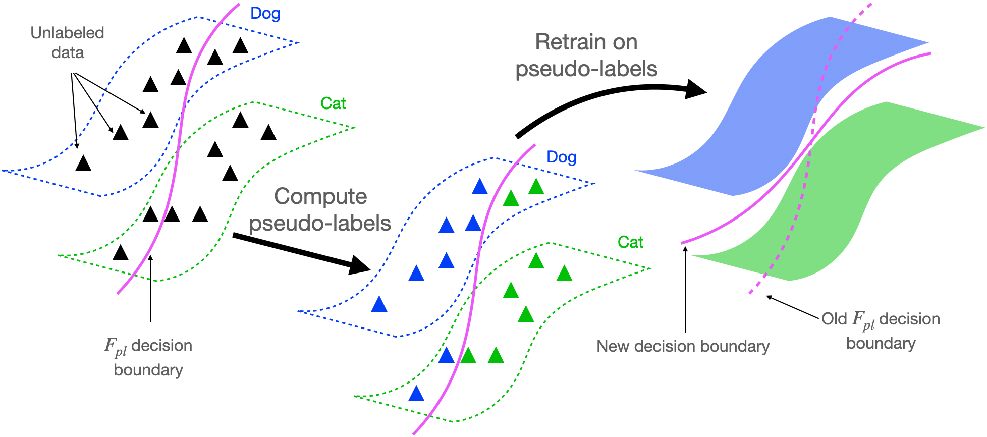
We will first provide a basic overview of self-training algorithms, which are the main focus of this blog post. The core idea is to use some pre-existing classifier (F_{pl}) (referred to as the “pseudo-labeler”) to make predictions (referred to as “pseudo-labels”) on a large unlabeled dataset, and then retrain a new model with the pseudo-labels. For example, in semi-supervised learning, the pseudo-labeler is obtained from training on a small labeled dataset, and is then used to predict pseudo-labels on a larger unlabeled dataset. A new classifier (F) is then retrained from scratch to fit the pseudo-labels, using additional regularization. In practice, (F) will often be more accurate than the original pseudo-labeler (F_{pl}) (Lee 2013). The self-training procedure is depicted below.
It is quite surprising that self-training can work so well in practice, given that we retrain on our own predictions, i.e. the pseudo-labels, but not the true labels. In the rest of this blogpost, we’ll share our theoretical analysis explaining why this is the case, showing that retraining in self-training provably improves accuracy compared to the original pseudo-labeler.
Our theoretical analysis focuses on pseudo-label-based self-training, but there are also other variants. For example, entropy minimization, which essentially trains on changing pseudo-labels produced by (F), rather than fixed pseudo-labels from (F_{pl}), can also be interpreted as self-training. Related analysis techniques apply to these algorithms (Cai et al. ‘21).
The importance of regularization for self-training
Before discussing core parts of our theory, we’ll first set up the analysis by demonstrating that regularization during the retraining phase is necessary for self-training to work well.
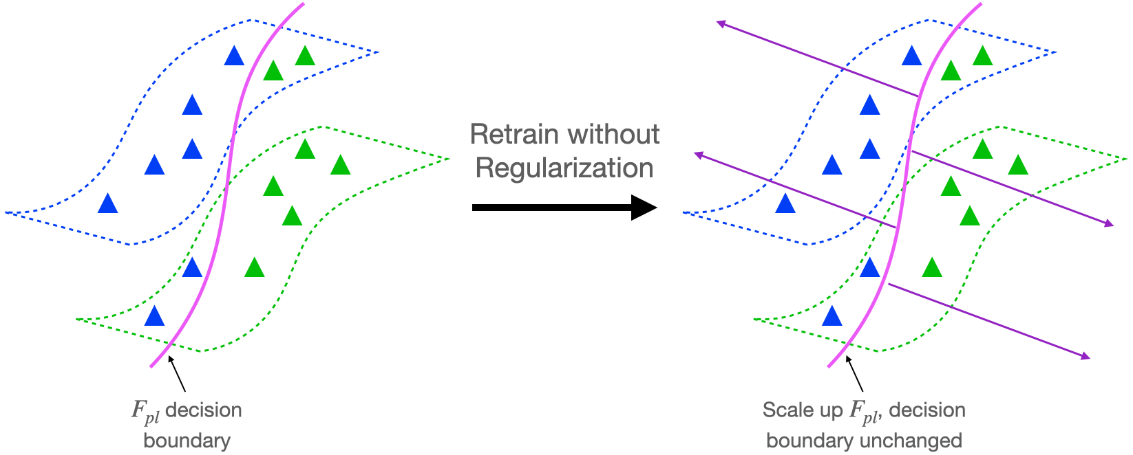
Let’s consider the retraining step of the self-training algorithm described above. Suppose we minimize the cross-entropy loss to fit the pseudo-labels, as is the case for deep networks. It’s possible to drive the unregularized cross-entropy loss to 0 by scaling up the predictions of (F_{pl}) to infinity. As depicted in Figure 2 below, this means that the retraining step won’t achieve any improvement over (F_{pl}) because the decision boundary will not change. This suggests that regularization might be necessary to have in our analysis if self-training is to lead to provable improvements over the pseudo-labeler.
Empirically, one technique which leads to substantial improvements after the retraining step is to encourage the classifier to have consistent predictions on neighboring pairs of examples. We refer to such methods as forms of input consistency regularization. In the literature, there are various ways to define “neighboring pairs”, for example, examples close in (ell_2) distance (Miyato et al., 2017, Shu et al., 2018), or examples which are different strong data augmentations of the same image (Xie et al., 2019, Berthelot et al., 2019, Xie et al., 2019, Sohn et al., 2020). Strong data augmentation, which applies stronger alterations to the input image than traditionally used in supervised learning, is also very useful for self-supervised contrastive learning, which we will analyze in the follow-up blog post. Our theoretical analysis considers a regularizer which is inspired by empirical work on input consistency regularization.
Key formulations for theoretical analysis
From the discussion above, it’s clear that in order to understand why self-training helps, we need a principled way to think about the regularizer for self-training. Input consistency regularization is effective in practice, but how do we abstract it so that the analysis is tractable? Furthermore, what properties of the data does the input consistency regularizer leverage in order to be effective? In the next section we’ll introduce the augmentation graph, a key concept that allows us to cleanly resolve both challenges. Building upon the augmentation graph, subsequent sections will formally introduce the regularizer and assumptions on the data.
Augmentation graph on the population data
We introduce the augmentation graph on the population data, a key concept which allows us to formalize the input consistency regularizer and motivates natural assumptions on the data distribution.
Intuitively, the augmentation graph is a graph with data points as vertices with the property that semantically similar data points will be connected by sequences of edges. We will consider the bipartite graph (G’) displayed in Figure 3 below, whose vertex set consists of all natural images (X) as well as the set (tilde{X}) of augmented versions of images in (X). The graph contains an edge (in pink) between (x in X) and (tilde{x} in tilde{X}) if (tilde{x}) is obtained by applying data augmentation to (x).
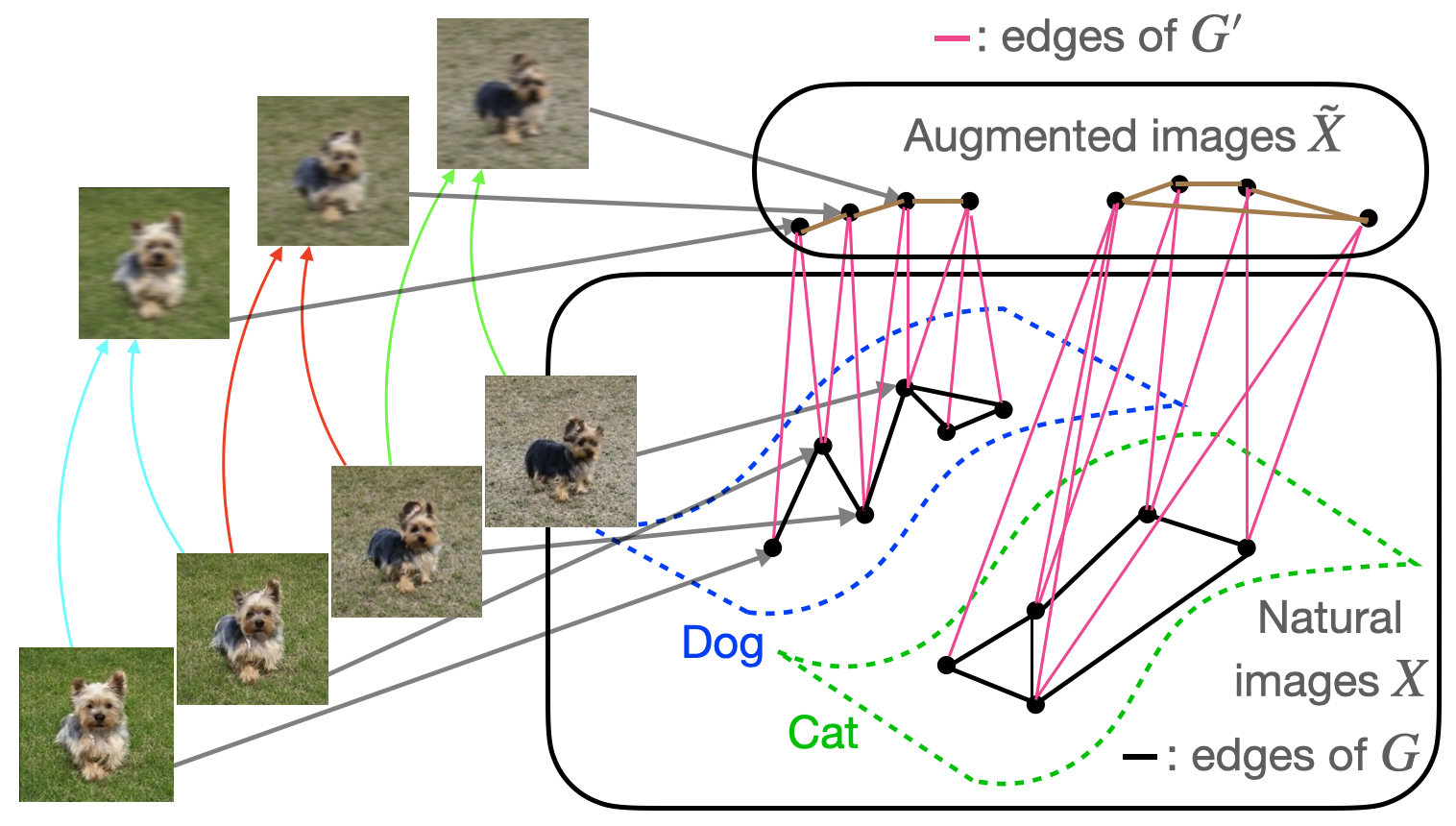
The analysis will be slightly simpler if we work with the graph (G) obtained by collapsing (G’) onto the vertex set (X). Edges of (G) are shown in black and connect vertices (x_1, x_2 in X) which share a common neighbor in (G’). Natural images (x_1, x_2 in X) are neighbors in (G) if and only if they share a common neighbor in (G’). In our next post on self-supervised contrastive learning algorithms, we will also consider the graph obtained by collapsing (G’) onto (tilde{X}), whose edges are shown in brown in the figure above.
For simplicity, we only consider unweighted graphs and focus on data augmentations which blur the image with small (ell_2)-bounded noise, although the augmentation graph can be constructed based on arbitrary types of data augmentation. The figure above shows examples of neighboring images in (G), with paired colored arrows pointing to their common augmentations in (tilde{X}). Note that by following edges in (G), it is possible to traverse a path between two rather different images, even though neighboring images in (G) are very similar and must have small (ell_2) distance from each other. An important point to stress is that (G) is a graph on the population data, not just the training set – this distinction is crucial for the type of assumptions we will make about (G).
Formalizing the regularizer
Now that we’ve defined the augmentation graph, let’s see how this concept helps us formulate our analysis. First, the augmentation graph motivates the following natural abstraction for the input consistency regularizer:
[R(F, x) = 1(F text{ predicts the same class on all examples in neighborhood } N(x)) tag{1}]In this definition, the neighborhood (N(x)) is the set of all (x’) such that (x) and (x’) are connected by an edge in the augmentation graph. The final population self-training objective which we will analyze is a sum of the regularizer and loss in fitting the pseudo-label and is closely related to empirically successful objectives such as in (Xie et al., 2019, Sohn et al., 2020).
[E_x[1(F(x) ne G_{pl}(x))] + lambda E_x[R(F, x)] tag{2}]Assumptions on the data
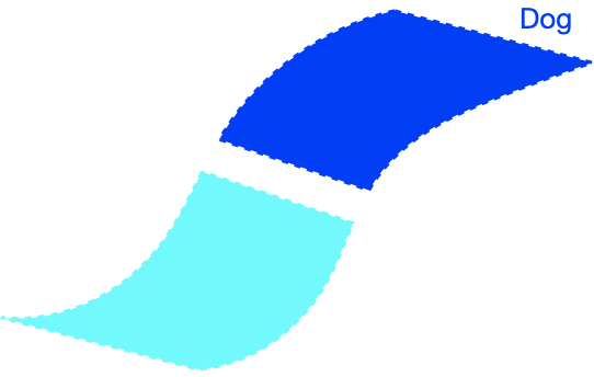
We will now perform a thought experiment to see why the regularizer is useful, and in doing so motivate two key assumptions for our analysis. Let’s consider an idealized case where the classifier has perfect input consistency, i.e., (R(F, x) = 0) for all (x). If the data satisfies an appropriate structure, enforcing perfect input consistency can be very advantageous, as visualized below.
The figure above demonstrates that if the dog class is connected in (G), enforcing perfect input consistency will ensure that the classifier makes the same prediction on all dogs. This is because the perfect input consistency ensures that the same label propagates through all neighborhoods of dog examples, eventually covering the entire class. This is beneficial for avoiding overfitting to incorrectly pseudolabeled examples.
There were two implicit properties of the data distribution in Figure 4 which ensured that the perfect input consistency was beneficial: 1) The dog class was connected in (G), and 2) The dog and cat classes were far apart. Figure 5 depicts failure cases where these conditions don’t hold, so the perfect input consistency does not help. The left shows that if the dog class is not connected in (G), perfect input consistency may not guarantee that the classifier predicts the same label throughout the class. The right shows that if the dog and cat classes are too close together, perfect input consistency would imply that the classifier cannot distinguish between the two classes.
Our main assumptions, described below, are natural formalizations of the conditions above.
Assumption 1 (Expansion within classes): The augmentation graph has good connectivity within classes. Formally, for any subset (S) of images within a ground-truth class, (P(N(S)) > cP(S)) for some (c > 1).
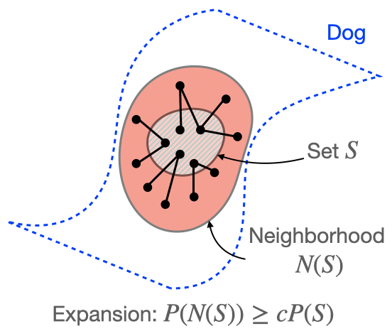
The figure above illustrates Assumption 1. In Assumption 1, (N(S)) refers to the neighborhood of (S), which contains (S) and the union of neighborhoods of examples in (S). We refer to Assumption 1 as the “expansion” assumption because it requires that the neighborhood of (S) must expand by a constant factor (c) in probability relative to (S) itself. We refer to the coefficient (c) as the expansion coefficient. Intuitively, larger (c) implies better connectivity because it means each set has a larger neighborhood. Related notions of expansion have been studied in the past in settings such as spectral graph theory [2,3], sampling and mixing time [4], combinatorial optimization [5], and even semi-supervised learning in a different co-training setting [1].
Assumption 2 (Separation between classes): There is separation between classes: the graph (G) does contains a very limited number of edges between different classes.
In the paper, we provide examples of distributions satisfying expansion and separation, and we believe that they are realistic characterizations of real data. One key point to reiterate is that these assumptions and the graph (G) are defined for population data. Indeed, it is not realistic to have properties such as expansion hold for the training set. If we were to attempt to build the graph (G) on only training examples, it would be completely disconnected because the probability of drawing two i.i.d. samples which happen to be neighbors (defined over (ell_2) distance) is exponentially small in the input dimension.
Main theoretical results
We now show that a model satisfying low self-training loss (2) will have good classification accuracy. Our main result is as follows:
Theorem 1 (informal): There exists a choice of input consistency regularization strength (lambda) such that if the pseudo-labeler satisfies a baseline level of accuracy, i.e., (text{Error}(G_{pl}) < 1/3), the minimizer (hat{F}) of the population objective (2) will satisfy:
[text{Error}(hat{F}) le frac{2}{c – 1} text{Error}(G_{pl})]In other words, assuming expansion and separation, self training provably leads to a more accurate classifier than the original pseudo-labeler! One of the main advantages of Theorem 1 is that it does not depend on the parameterization of (F), and, in particular, holds when (F) is a deep network. Furthermore, in the domain adaptation setting, we do not require any assumptions about the relationship between the source and target domain, as long as the pseudo-labeler hits the baseline accuracy level. Prior analyses of self-training were restricted to linear models (e.g., Kumar et al. 2020, Chen et al. 2020), or domain adaptation settings where the domain shift is assumed to be very small (Kumar et al. 2020).
An interesting property of the bound is that it improves as the coefficient (c) in the expansion assumption gets larger. Recall that (c) essentially serves as a quantifier for how connected the augmentation graph is within each class, and larger (c) indicates more connectivity. Intuitively, connectivity can improve the bound by strengthening the impact of the input consistency regularizer.
One way to improve the graph connectivity is to use stronger data augmentations. In fact, this approach has worked very well empirically: algorithms like FixMatch and Noisy Student achieve state-of-the-art semi-supervised learning performance by using data augmentation which alters the images much more strongly than in standard supervised learning. Theorem 1 suggests an explanation for why strong data augmentation is so helpful: it leads to a larger (c) and a smaller bound. However, one does need to be careful to not increase augmentation strength by too much – using too strong data augmentation could make it so that our Assumption 2 that ground truth classes are separated would no longer hold.
The proof of Theorem 1 relies on the intuition conveyed in the previous subsection. Recall that the goal is to show that retraining on pseudo-labels can lead to a classifier which corrects some of the mistakes in the pseudo-labels. The reason why the classifier can ignore some incorrect pseudo-labels is that the input consistency regularization term in (2) encourages the classifier to predict the same label on neighboring examples. Thus, we can hope that the correctly pseudo-labeled examples will propagate their labels to incorrectly pseudo-labeled neighbors, leading to a denoising effect on these neighbors. We can make this intuition rigorous by leveraging the expansion assumption (Assumption 1).
The main result of Theorem 1 and our assumptions were phrased for population data, but it’s not too hard to transform Theorem 1 into accuracy guarantees for optimizing (2) on a finite training set. The key observation is that even if we only optimize the training version of (2), because of generalization, the population loss will also be small, which is actually sufficient for achieving the accuracy guarantees of Theorem 1.
Conclusion
In this blog post, we discussed why self-training on unlabeled data provably improves accuracy. We built an augmentation graph on the data such that nearby examples are connected with an edge. We assumed that two examples in the same class can be connected via a sequence of edges in the graph. Under this assumption, we showed that self-training with regularization improves upon the accuracy of the pseudo-labeler by enforcing each connected subgraph to have the same label. One limitation is that the analysis only works when the classes are fine-grained, so that each class forms its own connected component in the augmentation graph. However, we can imagine scenarios where one large class is a union of smaller, sparsely connected subclasses. In these cases, our assumptions may not hold. Our follow-up blog post on contrastive learning will show how to deal with this case.
This blog post was based on the paper Theoretical Analysis of Self-Training with Deep Networks on Unlabeled Data.
Additional references
- Balcan MF, Blum A, Yang K. Co-training and expansion: Towards bridging theory and practice. Advances in neural information processing systems; 2005.
- Cheeger J. A lower bound for the smallest eigenvalue of the Laplacian. Problems in analysis; 2015.
- Chung FR, Graham FC. Spectral graph theory. American Mathematical Soc.; 1997.
- Kannan R, Lovász L, Simonovits M. Isoperimetric problems for convex bodies and a localization lemma. Discrete & Computational Geometry; 1995.
- Mohar B, Poljak S. Eigenvalues and the max-cut problem. Czechoslovak Mathematical Journal; 1990.
Case Study: Amazon Ads Uses PyTorch and AWS Inferentia to Scale Models for Ads Processing
Amazon Ads uses PyTorch, TorchServe, and AWS Inferentia to reduce inference costs by 71% and drive scale out.
Amazon Ads helps companies build their brand and connect with shoppers through ads shown both within and beyond Amazon’s store, including websites, apps, and streaming TV content in more than 15 countries. Businesses and brands of all sizes, including registered sellers, vendors, book vendors, Kindle Direct Publishing (KDP) authors, app developers, and agencies can upload their own ad creatives, which can include images, video, audio, and, of course, products sold on Amazon.

To promote an accurate, safe, and pleasant shopping experience, these ads must comply with content guidelines. For example, ads cannot flash on and off, products must be featured in an appropriate context, and images and text should be appropriate for a general audience. To help ensure that ads meet the required policies and standards, we needed to develop scalable mechanisms and tools.
As a solution, we used machine learning (ML) models to surface ads that might need revision. As deep neural networks flourished over the past decade, our data science team began exploring more versatile deep learning (DL) methods capable of processing text, images, audio, or video with minimal human intervention. To that end, we’ve used PyTorch to build computer vision (CV) and natural language processing (NLP) models that automatically flag potentially non-compliant ads. PyTorch is intuitive, flexible, and user-friendly, and has made our transition to using DL models seamless. Deploying these new models on AWS Inferentia-based Amazon EC2 Inf1 instances, rather than on GPU-based instances, reduced our inference latency by 30 percent and our inference costs by 71 percent for the same workloads.
Transition to deep learning
Our ML systems paired classical models with word embeddings to evaluate ad text. But our requirements evolved, and as the volume of submissions continued to expand, we needed a method nimble enough to scale along with our business. In addition, our models must be fast and serve ads within milliseconds to provide an optimal customer experience.
Over the last decade, DL has become very popular in numerous domains, including natural language, vision, and audio. Because deep neural networks channel data sets through many layers — extracting progressively higher-level features — they can make more nuanced inferences than classical ML models. Rather than simply detecting prohibited language, for example, a DL model can reject an ad for making false claims.
In addition, DL techniques are transferable– a model trained for one task can be adapted to carry out a related task. For instance, a pre-trained neural network can be optimized to detect objects in images and then fine-tuned to identify specific objects that are not allowed to be displayed in an ad.
Deep neural networks can automate two of classical ML’s most time-consuming steps: feature engineering and data labeling. Unlike traditional supervised learning approaches, which require exploratory data analysis and hand-engineered features, deep neural networks learn the relevant features directly from the data. DL models can also analyze unstructured data, like text and images, without the preprocessing necessary in ML. Deep neural networks scale effectively with more data and perform especially well in applications involving large data sets.
We chose PyTorch to develop our models because it helped us maximize the performance of our systems. With PyTorch, we can serve our customers better while taking advantage of Python’s most intuitive concepts. The programming in PyTorch is object-oriented: it groups processing functions with the data they modify. As a result, our codebase is modular, and we can reuse pieces of code in different applications. In addition, PyTorch’s eager mode allows loops and control structures and, therefore, more complex operations in the model. Eager mode makes it easy to prototype and iterate upon our models, and we can work with various data structures. This flexibility helps us update our models quickly to meet changing business requirements.
“Before this, we experimented with other frameworks that were “Pythonic,” but PyTorch was the clear winner for us here.” said Yashal Kanungo, Applied Scientist. “Using PyTorch was easy because the structure felt native to Python programming, which the data scientists were very familiar with”.
Training pipeline
Today, we build our text models entirely in PyTorch. To save time and money, we often skip the early stages of training by fine-tuning a pre-trained NLP model for language analysis. If we need a new model to evaluate images or video, we start by browsing PyTorch’s torchvision library, which offers pretrained options for image and video classification, object detection, instance segmentation, and pose estimation. For specialized tasks, we build a custom model from the ground up. PyTorch is perfect for this, because eager mode and the user-friendly front end make it easy to experiment with different architectures.
To learn how to finetune neural networks in PyTorch, head to this tutorial.
Before we begin training, we optimize our model’s hyperparameters, the variables that define the network architecture (for example, the number of hidden layers) and training mechanics (such as learning rate and batch size). Choosing appropriate hyperparameter values is essential, because they will shape the training behavior of the model. We rely on the Bayesian search feature in SageMaker, AWS’s ML platform, for this step. Bayesian search treats hyperparameter tuning as a regression problem: It proposes the hyperparameter combinations that are likely to produce the best results and runs training jobs to test those values. After each trial, a regression algorithm determines the next set of hyperparameter values to test, and performance improves incrementally.
We prototype and iterate upon our models using SageMaker Notebooks. Eager mode lets us prototype models quickly by building a new computational graph for each training batch; the sequence of operations can change from iteration to iteration to accommodate different data structures or to jibe with intermediate results. That frees us to adjust the network during training without starting over from scratch. These dynamic graphs are particularly valuable for recursive computations based on variable sequence lengths, such as the words, sentences, and paragraphs in an ad that are analyzed with NLP.
When we’ve finalized the model architecture, we deploy training jobs on SageMaker. PyTorch helps us develop large models faster by running numerous training jobs at the same time. PyTorch’s Distributed Data Parallel (DDP) module replicates a single model across multiple interconnected machines within SageMaker, and all the processes run forward passes simultaneously on their own unique portion of the data set. During the backward pass, the module averages the gradients of all the processes, so each local model is updated with the same parameter values.
Model deployment pipeline
When we deploy the model in production, we want to ensure lower inference costs without impacting prediction accuracy. Several PyTorch features and AWS services have helped us address the challenge.
The flexibility of a dynamic graph enriches training, but in deployment we want to maximize performance and portability. An advantage of developing NLP models in PyTorch is that out of the box, they can be traced into a static sequence of operations by TorchScript, a subset of Python specialized for ML applications. Torchscript converts PyTorch models to a more efficient, production-friendly intermediate representation (IR) graph that is easily compiled. We run a sample input through the model, and TorchScript records the operations executed during the forward pass. The resulting IR graph can run in high-performance environments, including C++ and other multithreaded Python-free contexts, and optimizations such as operator fusion can speed up the runtime.
Neuron SDK and AWS Inferentia powered compute
We deploy our models on Amazon EC2 Inf1 instances powered by AWS Inferentia, Amazon’s first ML silicon designed to accelerate deep learning inference workloads. Inferentia has shown to reduce inference costs by up to 70% compared to Amazon EC2 GPU-based instances.
We used the AWS Neuron SDK — a set of software tools used with Inferentia — to compile and optimize our models for deployment on EC2 Inf1 instances.
The code snippet below shows how to compile a Hugging Face BERT model with Neuron. Like torch.jit.trace(), neuron.trace() records the model’s operations on an example input during the forward pass to build a static IR graph.
import torch
from transformers import BertModel, BertTokenizer
import torch.neuron
tokenizer = BertTokenizer.from_pretrained("path to saved vocab")
model = BertModel.from_pretrained("path to the saved model", returned_dict=False)
inputs = tokenizer ("sample input", return_tensor="pt")
neuron_model = torch.neuron.trace(model,
                                  example_inputs = (inputs['input_ids'], inputs['attention_mask']),
                                  verbose = 1)
output = neuron_model(*(inputs['input_ids'], inputs['attention_mask']))
Autocasting and recalibration
Under the hood, Neuron optimizes our models for performance by autocasting them to a smaller data type. As a default, most applications represent neural network values in the 32-bit single-precision floating point (FP32) number format. Autocasting the model to a 16-bit format — half-precision floating point (FP16) or Brain Floating Point (BF16) — reduces a model’s memory footprint and execution time. In our case, we decided to use FP16 to optimize for performance while maintaining high accuracy.
Autocasting to a smaller data type can, in some cases, trigger slight differences in the model’s predictions. To ensure that the model’s accuracy is not affected, Neuron compares the performance metrics and predictions of the FP16 and FP32 models. When autocasting diminishes the model’s accuracy, we can tell the Neuron compiler to convert only the weights and certain data inputs to FP16, keeping the rest of the intermediate results in FP32. In addition, we often run a few iterations with the training data to recalibrate our autocasted models. This process is much less intensive than the original training.
Deployment
To analyze multimedia ads, we run an ensemble of DL models. All ads uploaded to Amazon are run through specialized models that assess every type of content they include: images, video and audio, headlines, texts, backgrounds, and even syntax, grammar, and potentially inappropriate language. The signals we receive from these models indicate whether or not an advertisement complies with our criteria.
Deploying and monitoring multiple models is significantly complex, so we depend on TorchServe, SageMaker’s default PyTorch model serving library. Jointly developed by Facebook’s PyTorch team and AWS to streamline the transition from prototyping to production, TorchServe helps us deploy trained PyTorch models at scale without having to write custom code. It provides a secure set of REST APIs for inference, management, metrics, and explanations. With features such as multi-model serving, model versioning, ensemble support, and automatic batching, TorchServe is ideal for supporting our immense workload. You can read more about deploying your Pytorch models on SageMaker with native TorchServe integration in this blog post.
In some use cases, we take advantage of PyTorch’s object-oriented programming paradigm to wrap multiple DL models into one parent object — a PyTorch nn.Module — and serve them as a single ensemble. In other cases, we use TorchServe to serve individual models on separate SageMaker endpoints, running on AWS Inf1 instances.
Custom handlers
We particularly appreciate that TorchServe allows us to embed our model initialization, preprocessing, inferencing, and post processing code in a single Python script, handler.py, which lives on the server. This script — the handler —preprocesses the un-labeled data from an ad, runs that data through our models, and delivers the resulting inferences to downstream systems. TorchServe provides several default handlers that load weights and architecture and prepare the model to run on a particular device. We can bundle all the additional required artifacts, such as vocabulary files or label maps, with the model in a single archive file.
When we need to deploy models that have complex initialization processes or that originated in third-party libraries, we design custom handlers in TorchServe. These let us load any model, from any library, with any required process. The following snippet shows a simple handler that can serve Hugging Face BERT models on any SageMaker hosting endpoint instance.
import torch
import torch.neuron
from ts.torch_handler.base_handler import BaseHandler
import transformers
from transformers import AutoModelForSequenceClassification,AutoTokenizer

class MyModelHandler(BaseHandler):
    def initialize(self, context):
        self.manifest = ctx.manifest
        properties = ctx.system_properties
        model_dir = properties.get("model_dir")
        serialized_file = self.manifest["model"]["serializedFile"]
        model_pt_path = os.path.join(model_dir, serialized_file)


        self.tokenizer = AutoTokenizer.from_pretrained(
                model_dir, do_lower_case=True
            )
        self.model = AutoModelForSequenceClassification.from_pretrained(
                    model_dir
                )

    def preprocess(self, data):

        input_text = data.get("data")
        if input_text is None:
            input_text = data.get("body")
            inputs = self.tokenizer.encode_plus(input_text, max_length=int(max_length), pad_to_max_length=True, add_special_tokens=True, return_tensors='pt')
        return inputs

    def inference(self,inputs):
        predictions = self.model(**inputs)
        return predictions

    def postprocess(self, output):
        return output
Batching
Hardware accelerators are optimized for parallelism, and batching — feeding a model multiple inputs in a single step — helps saturate all available capacity, typically resulting in higher throughputs. Excessively high batch sizes, however, can increase latency with minimal improvement in throughputs. Experimenting with different batch sizes helps us identify the sweet spot for our models and hardware accelerator. We run experiments to determine the best batch size for our model size, payload size, and request traffic patterns.
The Neuron compiler now supports variable batch sizes. Previously, tracing a model hardcoded the predefined batch size, so we had to pad our data, which can waste compute, slow throughputs, and exacerbate latency. Inferentia is optimized to maximize throughput for small batches, reducing latency by easing the load on the system.
Parallelism
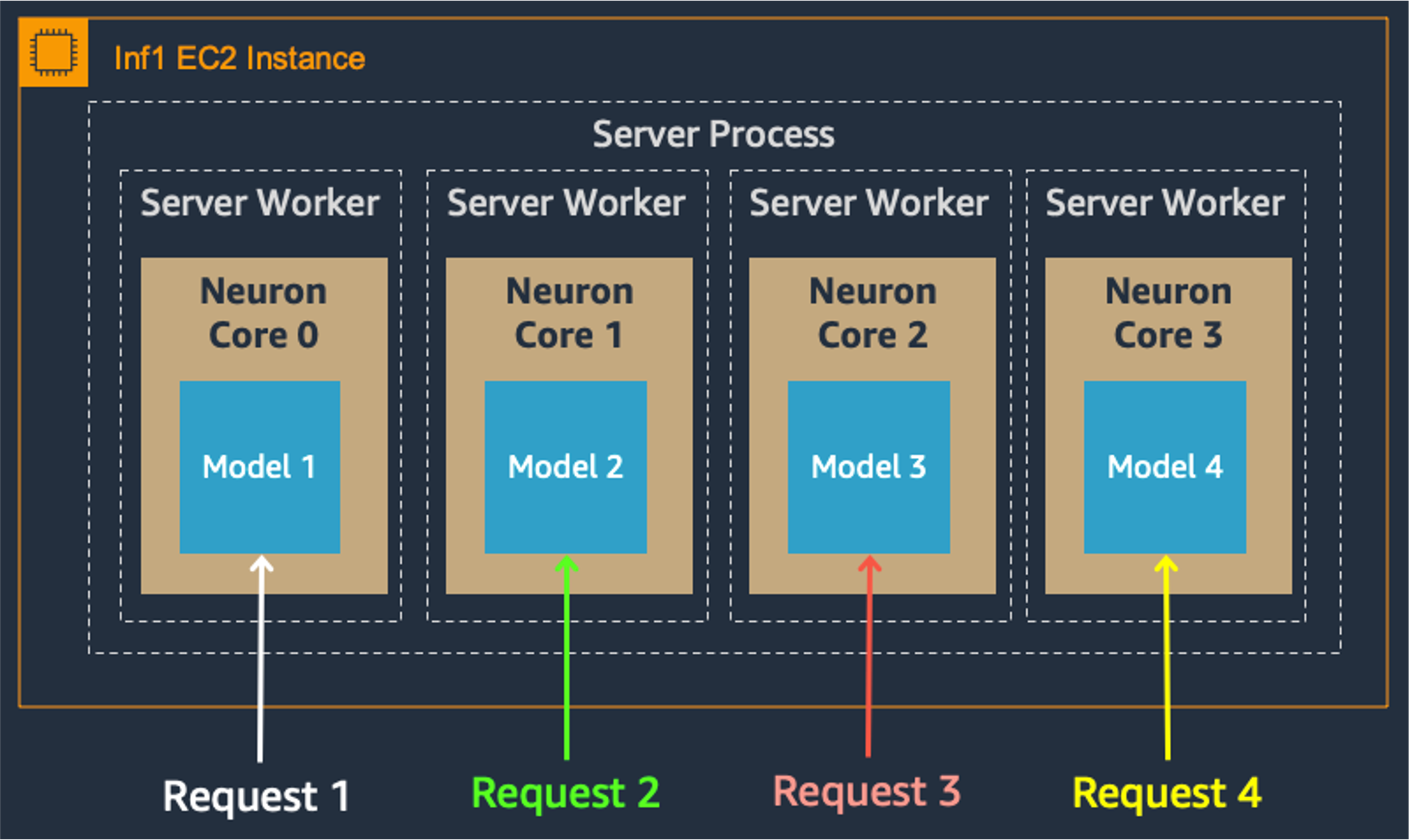
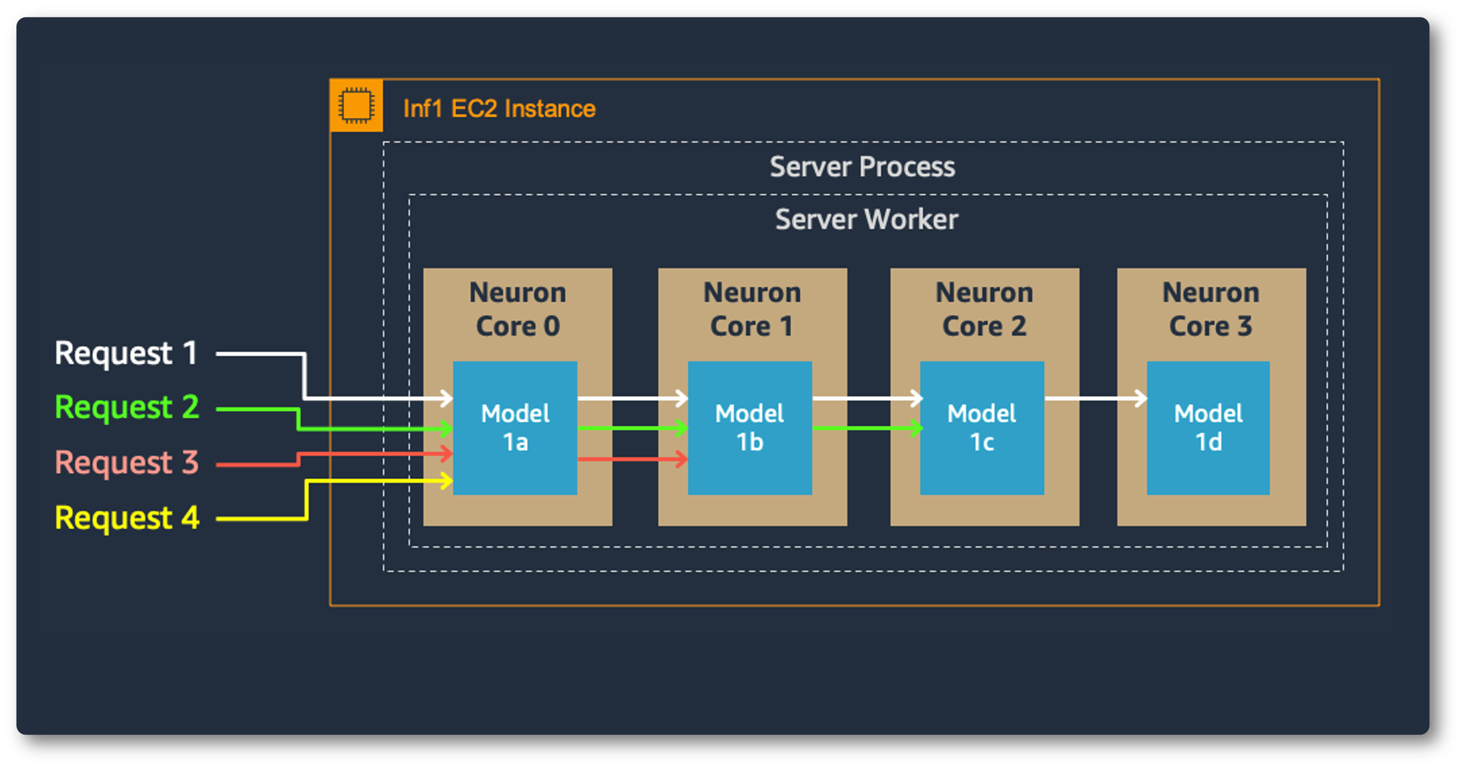
Model parallelism on multi-cores also improves throughput and latency, which is crucial for our heavy workloads. Each Inferentia chip contains four NeuronCores that can either run separate models simultaneously or form a pipeline to stream a single model. In our use case, the data parallel configuration offers the highest throughput at the lowest cost, because it scales out concurrent processing requests.
Data Parallel:
Model Parallel:
Monitoring
It is critical that we monitor the accuracy of our inferences in production. Models that initially make good predictions can eventually degrade in deployment as they are exposed to a wider variety of data. This phenomenon, called model drift, usually occurs when the input data distributions or the prediction targets change.
We use SageMaker Model Monitor to track parity between the training and production data. Model Monitor notifies us when predictions in production begin to deviate from the training and validation results. Thanks to this early warning, we can restore accuracy — by retraining the model if necessary — before our advertisers are affected. To track performance in real time, Model Monitor also sends us metrics about the quality of predictions, such as accuracy, F-scores, and the distribution of the predicted classes.
To determine if our application needs to scale, TorchServe logs resource utilization metrics for the CPU, Memory, and Disk at regular intervals; it also records the number of requests received versus the number served. For custom metrics, TorchServe offers a Metrics API.
A rewarding result
Our DL models, developed in PyTorch and deployed on Inferentia, sped up our ads analysis while cutting costs. Starting with our first explorations in DL, programming in PyTorch felt natural. Its user-friendly features helped smooth the course from our early experiments to the deployment of our multimodal ensembles. PyTorch lets us prototype and build models quickly, which is vital as our advertising service evolves and expands. For an added benefit, PyTorch works seamlessly with Inferentia and our AWS ML stack. We look forward to building more use cases with PyTorch, so we can continue to serve our clients accurate, real-time results.