Monthly Archives: February 2022

This is a guest post by Kustomer’s Senior Software & Machine Learning Engineer, Ian Lantzy, and AWS team Umesh Kalaspurkar, Prasad Shetty, and Jonathan Greifenberger.

In Kustomer’s own words, “Kustomer is the omnichannel SaaS CRM platform reimagining enterprise customer service to deliver standout experiences. Built with intelligent automation, we scale to meet the needs of any contact center and business by unifying data from multiple sources and enabling companies to deliver effortless, consistent, and personalized service and support through a single timeline view.”

Kustomer wanted the ability to rapidly analyze large volumes of support communications for their business customers — customer experience and service organizations — and automate discovery of information such as the end-customer’s intent, customer service issue, and other relevant insights related to the consumer. Understanding these characteristics can help CX organizations manage thousands of in-bound support emails by automatically classifying and categorizing the content. Kustomer leverages Amazon SageMaker to manage the analysis of the incoming support communications via their AI based Kustomer IQ platform. Kustomer IQ’s Conversation Classification service is able to contextualize conversations and automate otherwise tedious and repetitive tasks, reducing agent distraction and the overall cost per contact. This and Kustomer’s other IQ services have increased productivity and automation for its business customers.

In this post, we talk about how Kustomer uses custom Docker images for SageMaker training and inference, which eases integration and streamlines the process. With this approach, Kustomer’s business customers are automatically classifying over 50k support emails each month with up to 70% accuracy.

Background and challenges

Kustomer uses a custom text classification pipeline for their Conversation Classification service. This helps them manage thousands of requests a day via automatic classification and categorization utilizing SageMaker’s training and inference orchestration. The Conversation Classification training engine uses custom Docker images to process data and train models using historical conversations and then predicts the topics, categories, or other custom labels a particular agent needs in order to classify the conversations. Then the prediction engine utilizes the trained models with another custom docker image to categorize conversations, which organizations use to automate reporting or route conversations to a specific team based on its topic.

The SageMaker categorization process starts by establishing a training and inference pipeline that can provide text classification and contextual recommendations. A typical setup would be implemented with serverless approaches like AWS Lambda for data preprocessing and postprocessing because it has a minimal provisioning requirement with an effective on-demand pricing model. However, using SageMaker with dependencies such as TensorFlow, NumPy, and Pandas can quickly increase the model package size, making the overall deployment process cumbersome and difficult to manage. Kustomer used custom Docker images to overcome these challenges.

Custom Docker images provide substantial advantages:

• Allows for larger compressed package sizes (over 10 GB), which can contain popular machine learning (ML) frameworks such as TensorFlow, MXNet, PyTorch, or others.
• Allows you to bring custom code or algorithms developed locally to Amazon SageMaker Studio notebooks for rapid iteration and model training.
• Avoids preprocessing delays caused in Lambda while unpacking deployment packages.
• Offers flexibility to integrate seamlessly with internal systems.
• Future compatibility and scalability make it easier to convert a service using Docker rather than having to package .zip files in a Lambda function.
• Reduces the turnaround time for a CI/CD deployment pipeline.
• Provides Docker familiarity within the team and ease of use.
• Provides access to data stores via APIs and a backend runtime.
• Offers better support for intervening for any preprocessing or postprocessing that Lambda would require a separate compute service for each process (such as training or deployment).

Solution overview

Categorization and labeling of support emails is a critical step in the customer support process. It allows companies to route conversations to the right teams, and understand at a high level what their customers are contacting them about. Kustomer’s business customers handle thousands of conversations every day, so classifying at scale is a challenge. Automating this process helps agents be more effective and provide more cohesive support, and helps their customers by connecting them with the right people faster.

The following diagram illustrates the solution architecture:

The Conversation Classification process starts with the business customer giving Kustomer permission to set up a training and inference pipeline that can help them with text classification and contextual recommendations. Kustomer exposes a user interface to their customers to monitor the training and inference process, which is implemented using SageMaker along with TensorFlow models and custom Docker images. The process of building and utilizing a classifier is split into five main workflows, which are coordinated by a worker service running on Amazon ECS. To coordinate the pipeline events and trigger the training and deployment of the model, the worker uses an Amazon SQS queue and integrates directly with SageMaker using the AWS-provided Node.js SDK. The workflows are:

• Data export
• Data preprocessing
• Training
• Deployment
• Inference

Data export

The data export process is run on demand and starts with an approval process from Kustomer’s business customer to confirm the use of email data for analysis. Data relevant to the classification process is captured via the initial email received from the end customer. For example, a support email typically contains the complete coherent thought of the problem with details about the issue. As part of the export process, the emails are collated from the data store (MongoDB and Amazon OpenSearch) and saved in Amazon Simple Storage Service (Amazon S3).

Data preprocessing

The data preprocessing stage cleans the dataset for training and inference workflows by stripping any HTML tags from customer emails and feeding them through multiple cleaning and sanitization steps to detect any malformed HTML. This process includes the use of Hugging Face tokenizers and transformers. When the cleansing process is complete, any additional custom tokens required for training are added to the output dataset.

During the preprocessing stage, a Lambda function invokes a custom Docker image. This image consists of a Python 3.8 slim base, the AWS Lambda Python Runtime Interface Client, and dependencies such as NumPy and Pandas. The custom Docker image is stored on Amazon Elastic Container Registry (Amazon ECR) and then fed through the CI/CD pipeline for deployment. The deployed Lambda function samples the data to generate three distinct datasets per classifier:

• Training – Used for the actual training process
• Validation – Used for validation during the TensorFlow training process
• Test – Used towards the end of the training process for metrics model comparisons

The generated output datasets are Pandas pickle files, which are stored in Amazon S3 to be used by the training stage.

Training

Kustomer’s custom training image utilizes a TensorFlow 2.7 GPU-optimized docker image as a base. Custom code, dependencies, and base models are included before the custom docker training image is uploaded to ECR. P3 instance types are used for the training process and using a GPU optimized base image helps to make the training process as efficient as possible. Amazon SageMaker is used with this custom docker image to train TensorFlow models that are then stored in S3. Custom metrics are also computed and saved to help with additional capabilities such as model comparisons and automatic retraining. Once the training stage is completed, the AI worker is notified and the business customer is able to start the deployment workflow.

Deployment

For the deployment workflow, a custom docker inference image is created using a TensorFlow serving base image (built specifically for fast inference). Additional code and dependencies like numPy, Pandas, custom NL, etc. are included to provide additional functionality, such as formatting & cleaning inputs before inference. FastAPI is also included as part of the custom image, and is used to provide the REST API endpoints for inference and health checks. SageMaker is then configured to deploy the TensorFlow models saved in S3 with the inference image onto compute optimized ml.c5 AWS instances to generate high-performance inference endpoints. Each endpoint is created for use by a single customer to isolate their models and data.

Inference

Once the deployment workflow is completed, the inference workflow takes over. All first inbound support emails are passed through the inference API for the deployed classifiers specific to that customer. The deployed classifiers then perform text classification on each of these emails, each generating classification labels for the customer.

Possible enhancements and customizations

Kustomer is considering expanding the solution with the following enhancements:

• Hugging Face DLCs – Kustomer currently uses TensorFlow’s base Docker images for the data preprocessing stage and plans to migrate to Hugging Face Deep Learning Containers (DLCs). This helps you start training models immediately, skipping the complicated process of building and optimizing your training environments from scratch. For more information, see Hugging Face on Amazon SageMaker.
• Feedback loop – You can implement a feedback loop using active learning or reinforcement learning techniques to increase the overall efficiency of the model.
• Integration with other internal systems – Kustomer wants the ability to integrate the text classification with other systems like Smart Suggestions, which is another Kustomer IQ service that looks through hundreds of shortcuts and suggest the shortcuts that are most relevant to a customer query, improving agent response times and performance.

Conclusion

In this post, we discussed how Kustomer uses custom Docker images for SageMaker training and inference, which eases integration and streamlines the process. We demonstrated how Kustomer leverages Lambda and SageMaker with custom Docker images that help implement the text classification process with preprocessing and postprocessing workflows. This provides flexibility for using larger images for model creation, training, and inference. Container image support for Lambda allows you to customize your function even more, opening up many new use cases for serverless ML. The solution takes advantage of several AWS services, including SageMaker, Lambda, Docker images, Amazon ECR, Amazon ECS, Amazon SQS, and Amazon S3.

If you want to learn more about Kustomer, we encourage you to visit the Kustomer website and explore their case studies.

Click here to start your journey with Amazon SageMaker. For hands-on experience, you can reference the Amazon SageMaker workshop.

About the Authors

Umesh Kalaspurkar is a New York based Solutions Architect for AWS. He brings more than 20 years of experience in design and delivery of Digital Innovation and Transformation projects, across enterprises and startups. He is motivated by helping customers identify and overcome challenges. Outside of work, Umesh enjoys being a father, skiing, and traveling.

Ian Lantzy is a Senior Software & Machine Learning engineer for Kustomer and specializes in taking machine learning research tasks and turning them into production services.

Prasad Shetty is a Boston-based Solutions Architect for AWS. He has built software products and has led modernizing and digital innovation in product and services across enterprises for over 20 years. He is passionate about driving cloud strategy and adoption, and leveraging technology to create great customer experiences. In his leisure time, Prasad enjoys biking and traveling.

Jonathan Greifenberger is a New York based Senior Account Manager for AWS with 25 years of IT industry experience. Jonathan leads a team that assists clients from various industries and verticals on their cloud adoption and modernization journey.

Read More

Predictive maintenance can be an effective way to prevent industrial machinery failures and expensive downtime by proactively monitoring the condition of your equipment, so you can be alerted to any anomalies before equipment failures occur. Installing sensors and the necessary infrastructure for data connectivity, storage, analytics, and alerting are the foundational elements for enabling predictive maintenance solutions. However, even after installing the ad hoc infrastructure, many companies use basic data analytics and simple modeling approaches that are often ineffective at detecting issues early enough to avoid downtime. Also, implementing a machine learning (ML) solution for your equipment can be difficult and time-consuming.

With Amazon Lookout for Equipment, you can automatically analyze sensor data for your industrial equipment to detect abnormal machine behavior—with no ML experience required. This means you can detect equipment abnormalities with speed and precision, quickly diagnose issues, and take action to reduce expensive downtime.

Lookout for Equipment analyzes the data from your sensors and systems, such as pressure, flow rate, RPMs, temperature, and power, to automatically train a model specific to your equipment based on your data. It uses your unique ML model to analyze incoming sensor data in real time and identifies early warning signs that could lead to machine failures. For each alert detected, Lookout for Equipment pinpoints which specific sensors are indicating the issue, and the magnitude of impact on the detected event.

With a mission to put ML in the hands of every developer, we want to present another add-on to Lookout for Equipment: an open-source Python toolbox that allows developers and data scientists to build, train, and deploy Lookout for Equipment models similarly to what you’re used to with Amazon SageMaker. This library is a wrapper on top of the Lookout for Equipment boto3 python API and is provided to kick start your journey with this service. Should you have any improvement suggestions or bugs to report, please file an issue against the toolbox GitHub repository.

In this post, we provide a step-by-step guide for using the Lookout for Equipment open-source Python toolbox from within a SageMaker notebook.

Environment setup

To use the open-source Lookout for Equipment toolbox from a SageMaker notebook, we need to grant the SageMaker notebook the necessary permissions for calling Lookout for Equipment APIs. For this post, we assume that you have already created a SageMaker notebook instance. For instructions, refer to Get Started with Amazon SageMaker Notebook Instances. The notebook instance is automatically associated with an execution role.

1. To find the role that is attached to the instance, select the instance on the SageMaker console.
   
2. On the next screen, scroll down to find the AWS Identity and Access Management (IAM) role attached to the instance in the Permissions and encryption section.
3. Choose the role to open the IAM console.
   

Next, we attach an inline policy to our SageMaker IAM role.

4. On the Permissions tab of the role you opened, choose Add inline policy.
   
5. On the JSON tab, enter the following code. We use a wild card action (lookoutequipment:*) for the service for demo purposes. For real use cases, provide only the required permissions to run the appropriate SDK API calls.

       {
           "Version": "2012-10-17",
           "Statement": [
               {
                   "Effect": "Allow",
                   "Action": [
                       "lookoutequipment:*"
                   ],
                   "Resource": "*"
               }
           ]
       }

6. Choose Review policy.
7. Provide a name for the policy and create the policy.

In addition to the preceding inline policy, on the same IAM role, we need to set up a trust relationship to allow Lookout for Equipment to assume this role. The SageMaker role already has the appropriate data access to Amazon Simple Storage Service (Amazon S3); allowing Lookout for Equipment to assume this role makes sure it has the same access to the data than your notebook. In your environment, you may already have a specific role ensuring Lookout for Equipment has access to your data, in which case you don’t need to adjust the trust relationship of this common role.

8. Inside our SageMaker IAM role on the Trust relationships tab, choose Edit trust relationship.
9. Under the policy document, replace the whole policy with the following code:

       {
           "Version": "2012-10-17",
           "Statement": [
               {
                   "Effect": "Allow",
                   "Principal": {
                       "Service": "lookoutequipment.amazonaws.com"
                   },
                   "Action": "sts:AssumeRole"
               }
           ]
       }

10. Choose Update trust policy.

Now we’re all set to use the Lookout for Equipment toolbox in our SageMaker notebook environment. The Lookout for Equipment toolbox is an open-source Python package that allows data scientists and software developers to easily build and deploy time series anomaly detection models using Lookout for Equipment. Let’s look at what you can achieve more easily thanks to the toolbox!

Dependencies

At the time of writing, the toolbox needs the following installed:

• Python(>=3.6)
• boto3 (>= 1.17.48)
• markdown
• numpy
• pandas
• pyarrow
• s3fs

After you satisfy these dependencies, you can install and launch the Lookout for Equipment toolbox with the following command from a Jupyter terminal:

pip install lookoutequipment

The toolbox is now ready to use. In this post, we demonstrate how to use the toolbox by training and deploying an anomaly detection model. A typical ML development lifecycle consists of building the dataset for training, training the model, deploying the model, and performing inference on the model. The toolbox is quite comprehensive in terms of the functionalities it provides, but in this post, we focus on the following capabilities:

• Prepare the dataset
• Train an anomaly detection model using Lookout for Equipment
• Build visualizations for your model evaluation
• Configure and start an inference scheduler
• Visualize scheduler inferences results

Let’s understand how we can use the toolbox for each of these capabilities.

Prepare the dataset

Lookout for Equipment requires a dataset to be created and ingested. To prepare the dataset, complete the following steps:

1. Before creating the dataset, we need to load a sample dataset and upload it to an Amazon Simple Storage Service (Amazon S3) bucket. In this post, we use the expander dataset:

   from lookoutequipment import dataset
   
   data = dataset.load_dataset(dataset_name='expander', target_dir='expander-data')
   dataset.upload_dataset('expander-data', bucket, prefix)

The returned data object represents a dictionary containing the following:

• • A training data DataFrame
  • A labels DataFrame
  • The training start and end datetimes
  • The evaluation start and end datetimes
  • A tags description DataFrame

The training and label data are uploaded from the target directory to Amazon S3 at the bucket/prefix location.

2. After uploading the dataset in S3, we create an object of LookoutEquipmentDataset class that manages the dataset:

   lookout_dataset = dataset.LookoutEquipmentDataset(
       dataset_name='my_dataset',
       access_role_arn=role_arn,
       component_root_dir=f's3://{bucket}/{prefix}training-data'
   )
   
   # creates the dataset
   lookout_dataset.create()

The access_role_arn supplied must have access to the S3 bucket where the data is present. You can retrieve the role ARN of the SageMaker notebook instance from the previous Environment setup section and add an IAM policy to grant access to your S3 bucket. For more information, see Writing IAM Policies: How to Grant Access to an Amazon S3 Bucket.

The component_root_dir parameter should indicate the location in Amazon S3 where the training data is stored.

After we launch the preceding APIs, our dataset has been created.

3. Ingest the data into the dataset:

   response = lookout_dataset.ingest_data(bucket, prefix + 'training-data/')

Now that your data is available on Amazon S3, creating a dataset and ingesting the data in it is just a matter of three lines of code. You don’t need to build a lengthy JSON schema manually; the toolbox detects your file structure and builds it for you. After your data is ingested, it’s time to move to training!

Train an anomaly detection model

After the data has been ingested in the dataset, we can start the model training process. See the following code:

from lookoutequipment import model

lookout_model = model.LookoutEquipmentModel(model_name='my_model', dataset_name='my_dataset')

lookout_model.set_time_periods(data['evaluation_start'],data['evaluation_end'],data['training_start'],data['training_end'])
lookout_model.set_label_data(bucket=bucket,prefix=prefix + 'label-data/',access_role_arn=role_arn)
lookout_model.set_target_sampling_rate(sampling_rate='PT5M')

#trigger training job
response = lookout_model.train()

#poll every 5 minutes to check the status of the training job
lookout_model.poll_model_training(sleep_time=300)

Before we launch the training, we need to specify the training and evaluation periods within the dataset. We also set the location in Amazon S3 where the labeled data is stored and set the sampling rate to 5 minutes. After we launch the training, the poll_model_training polls the training job status every 5 minutes until the training is successful.

The training module of the Lookout for Equipment toolbox allows you to train a model with less than 10 lines of code. It builds all the length creation request strings needed by the low-level API on your behalf, removing the need for you to build long, error-prone JSON documents.

After the model is trained, we can either check the results over the evaluation period or configure an inference scheduler using the toolbox.

Evaluate a trained model

After a model is trained, the DescribeModel API from Lookout for Equipment records the metrics associated to the training. This API returns a JSON document with two fields of interest to plot the evaluation results: labeled_ranges and predicted_ranges, which contain the known and predicted anomalies in the evaluation range, respectively. The toolbox provides utilities to load these in a Pandas DataFrame instead:

from lookoutequipment import evaluation

LookoutDiagnostics = evaluation.LookoutEquipmentAnalysis(model_name='my_model', tags_df=data['data'])

predicted_ranges = LookoutDiagnostics.get_predictions()
labels_fname = os.path.join('expander-data', 'labels.csv')
labeled_range = LookoutDiagnostics.get_labels(labels_fname)

The advantage of loading the ranges in a DataFrame is that we can create nice visualizations by plotting one of the original time series signals and add an overlay of the labeled and predicted anomalous events by using the TimeSeriesVisualization class of the toolbox:

from lookoutequipment import plot

TSViz = plot.TimeSeriesVisualization(timeseries_df=data['data'], data_format='tabular')
TSViz.add_signal(['signal-001'])
TSViz.add_labels(labeled_range)
TSViz.add_predictions([predicted_ranges])
TSViz.add_train_test_split(data['evaluation_start'])
TSViz.add_rolling_average(60*24)
TSViz.legend_format = {'loc': 'upper left', 'framealpha': 0.4, 'ncol': 3}
fig, axis = TSViz.plot()

These few lines of code generate a plot with the following features:

• A line plot for the signal selected; the part used for training the model appears in blue while the evaluation part is in gray
• The rolling average appears as a thin red line overlaid over the time series
• The labels are shown in a green ribbon labelled “Known anomalies” (by default)
• The predicted events are shown in a red ribbon labelled “Detected events”

The toolbox performs all the heavy lifting of locating, loading, and parsing the JSON files while providing ready-to-use visualizations that further reduce the time to get insights from your anomaly detection models. At this stage, the toolbox lets you focus on interpreting the results and taking actions to deliver direct business value to your end-users. In addition to these time series visualizations, the SDK provides other plots such as a histogram comparison of the values of your signals between normal and abnormal times. To learn more about the other visualization capabilities you can use right out of the box, see the Lookout for Equipment toolbox documentation.

Schedule inference

Let’s see how we can schedule inferences using the toolbox:

from lookout import scheduler

#prepare dummy inference data
dataset.prepare_inference_data(
    root_dir='expander-data',
    sample_data_dict=data,
    bucket=bucket,
    prefix=prefix
)

#setup the scheduler
lookout_scheduler = scheduler.LookoutEquipmentScheduler(scheduler_name='my_scheduler',model_name='my_model')
scheduler_params = {
                    'input_bucket': bucket,
                    'input_prefix': prefix + 'inference-data/input/',
                    'output_bucket': bucket,
                    'output_prefix': prefix + 'inference-data/output/',
                    'role_arn': role_arn,
                    'upload_frequency': 'PT5M',
                    'delay_offset': None,
                    'timezone_offset': '+00:00',
                    'component_delimiter': '_',
                    'timestamp_format': 'yyyyMMddHHmmss'
                    }
                    
lookout_scheduler.set_parameters(**scheduler_params)
response = lookout_scheduler.create()

This code creates a scheduler that processes one file every 5 minutes (matching the upload frequency set when configuring the scheduler). After 15 minutes or so, we should have some results available. To get these results from the scheduler in a Pandas DataFrame, we just have to run the following command:

results_df = lookout_scheduler.get_predictions()

From here, we can also plot the feature importance for a prediction using the visualization APIs of the toolbox:

event_details = pd.DataFrame(results_df.iloc[0, 1:]).reset_index()
fig, ax = plot.plot_event_barh(event_details)

It produces the following feature importance visualization on the sample data.

The toolbox also provides an API to stop the scheduler. See the following code snippet:

scheduler.stop()

Clean up

To delete all the artifacts created previously, we can call the delete_dataset API with the name of our dataset:

dataset.delete_dataset(dataset_name='my_dataset', delete_children=True, verbose=True)

Conclusion

When speaking to industrial and manufacturing customers, a common challenge we hear regarding taking advantage of AI and ML is the sheer amount of customization and specific development and data science work needed to obtain reliable and actionable results. Training anomaly detection models and getting actionable forewarning for many different industrial machineries is a prerequisite to reduce maintenance effort, reduce rework or waste, increase product quality, and improve overall equipment efficiency (OEE) or product lines. Until now, this required a massive amount of specific development work, which is hard to scale and maintain over time.

Amazon Applied AI services such as Lookout for Equipment enables manufacturers to build AI models without having access to a versatile team of data scientists, data engineers, and process engineers. Now, with the Lookout for Equipment toolbox, your developers can further reduce the time needed to explore insights in your time series data and take action. This toolbox provides an easy-to-use, developer-friendly interface to quickly build anomaly detection models using Lookout for Equipment. The toolbox is open source and all the SDK code can be found on the amazon-lookout-for-equipment-python-sdk GitHub repo. It’s also available as a PyPi package.

This post covers only few of the most important APIs. Interested readers can check out the toolbox documentation to look at more advanced capabilities of the toolbox. Give it a try, and let us know what you think in comments!

About the Authors

Vikesh Pandey is a Machine Learning Specialist Specialist Solutions Architect at AWS, helping customers in the UK and wider EMEA region design and build ML solutions. Outside of work, Vikesh enjoys trying out different cuisines and playing outdoor sports.

Ioan Catana is an Artificial Intelligence and Machine Learning Specialist Solutions Architect at AWS. He helps customers develop and scale their ML solutions in the AWS Cloud. Ioan has over 20 years of experience, mostly in software architecture design and cloud engineering.

Michaël Hoarau is an AI/ML Specialist Solutions Architect at AWS who alternates between data scientist and machine learning architect, depending on the moment. He is passionate about bringing the power of AI/ML to the shop floors of his industrial customers and has worked on a wide range of ML use cases, ranging from anomaly detection to predictive product quality or manufacturing optimization. When not helping customers develop the next best machine learning experiences, he enjoys observing the stars, traveling, or playing the piano.

Read More

Amazon SageMaker is a managed service that makes it easy to build, train, and deploy machine learning (ML) models. Data scientists use SageMaker training jobs to easily train ML models; you don’t have to worry about managing compute resources, and you pay only for the actual training time. Data ingestion is an integral part of any training pipeline, and SageMaker training jobs support a variety of data storage and input modes to suit a wide range of training workloads.

This post helps you choose the best data source for your SageMaker ML training use case. We introduce the data sources options that SageMaker training jobs support natively. For each data source and input mode, we outline its ease of use, performance characteristics, cost, and limitations. To help you get started quickly, we provide the diagram with a sample decision flow that you can follow based on your key workload characteristics. Lastly, we perform several benchmarks for realistic training scenarios to demonstrate the practical implications on the overall training cost and performance.

Native SageMaker data sources and input modes

Reading training data easily and flexibly in a performant way is a common recurring concern for ML training. SageMaker simplifies data ingestion with a selection of efficient, high-throughput data ingestion mechanisms called data sources and their respective input modes. This allows you to decouple training code from the actual data source, automatically mount file systems, read with high performance, easily turn on data sharding between GPUs and instances to enable data parallelism, and auto shuffle data at the start of each epoch.

The SageMaker training ingestion mechanism natively integrates with three AWS managed storage services:

• Amazon Simple Storage Service (Amazon S3) is an object storage service that offers industry-leading scalability, data availability, security, and performance.
• Amazon FSx for Lustre is a fully managed shared storage with the scalability and performance of the popular Lustre file system. It’s usually linked to an existing S3 bucket.
• Amazon Elastic File System (Amazon EFS) is a general purpose, scalable, and highly available shared file system with multiple price tiers. Amazon EFS is serverless and automatically grows and shrinks as you add and remove files.

SageMaker training allows your training script to access datasets stored on Amazon S3, FSx for Lustre, or Amazon EFS, as if it were available on a local file system (via a POSIX-compliant file system interface).

With Amazon S3 as a data source, you can choose between File mode, FastFile mode, and Pipe mode:

• File mode – SageMaker copies a dataset from Amazon S3 to the ML instance storage, which is an attached Amazon Elastic Block Store (Amazon EBS) volume or NVMe SSD volume, before your training script starts.
• FastFile mode – SageMaker exposes a dataset residing in Amazon S3 as a POSIX file system on the training instance. Dataset files are streamed from Amazon S3 on demand as your training script reads them.
• Pipe mode – SageMaker streams a dataset residing in Amazon S3 to the ML training instance as a Unix pipe, which streams from Amazon S3 on demand as your training script reads the data from the pipe.

With FSx for Lustre or Amazon EFS as a data source, SageMaker mounts the file system before your training script starts.

Training input channels

When launching an SageMaker training job, you can specify up to 20 managed training input channels. You can think of channels as an abstraction unit to tell the training job how and where to get the data that is made available to the algorithm code to read from a file system path (for example, /opt/ml/input/data/input-channel-name) on the ML instance. The selected training channels are captured as part of the training job metadata in order to enable a full model lineage tracking for use cases such as reproducibility of training jobs or model governance purposes.

To use Amazon S3 as your data source, you define a TrainingInput to specify the following:

• Your input mode (File, FastFile, or Pipe mode)
• Distribution and shuffling configuration
• An S3DataType as one of three methods for specifying objects in Amazon S3 that make up your dataset:
  • S3Prefix (all objects under the S3 prefix)
  • Manifest file (a list of S3 objects)
  • Augmented manifest file (a list of S3 objects and their respective labels)

Alternatively, for FSx for Lustre or Amazon EFS, you define a FileSystemInput.

The following diagram shows five training jobs, each configured with a different data source and input mode combination:

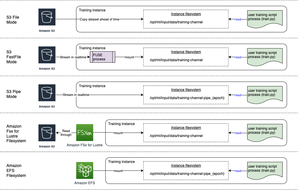
Data sources and input modes

The follow sections provide a deep dive into the differences between Amazon S3 (File mode, FastFile mode, and Pipe mode), FSx for Lustre, and Amazon EFS as SageMaker ingestion mechanisms.

Amazon S3 File mode

File mode is the default input mode (if you didn’t explicitly specify one), and it’s the more straightforward to use. When you use this input option, SageMaker downloads the dataset from Amazon S3 into the ML training instance storage (Amazon EBS or local NVMe depending on the instance type) on your behalf before launching model training, so that the training script can read the dataset from the local file system. In this case, the instance must have enough storage space to fit the entire dataset.

You configure the dataset for File mode by providing either an S3 prefix, manifest file, or augmented manifest file.

You should use an S3 prefix when all your dataset files are located within a common S3 prefix (subfolders are okay).

The manifest file lists the files comprising your dataset. You typically use a manifest when a data preprocessing job emits a manifest file, or when your dataset files are spread across multiple S3 prefixes. An augmented manifest is a JSON line file, where each line contains a list of attributes, such as a reference to a file in Amazon S3, alongside additional attributes, mostly labels. Its use cases are similar to that of a manifest.

File mode is compatible with SageMaker local mode (starting a SageMaker training container interactively in seconds). For distributed training, you can shard the dataset across multiple instances with the ShardedByS3Key option.

File mode download speed depends on dataset size, average file size, and number of files. For example, the larger the dataset is (or the more files it has), the longer the downloading stage is, during which the compute resource of the instance remains effectively idle. When training with Spot Instances, the dataset is downloaded each time the job resumes after a Spot interruption. Typically, data downloading takes place at approximately 200 MB/s for large files (for example, 5 minutes/50 GB). Whether this startup overhead is acceptable primarily depends on the overall duration of your training job, because a longer training phase means a proportionally smaller download phase.

Amazon S3 FastFile mode

FastFile mode exposes S3 objects via a POSIX-compliant file system interface, as if the files were available on the local disk of your training instance, and streams their content on demand when data is consumed by the training script. This means your dataset no longer needs to fit into the training instance storage space, and you don’t need to wait for the dataset to be downloaded to the training instance before training can start.

To facilitate this, SageMaker lists all the object metadata stored under the specified S3 prefix before your training script runs. This metadata is used to create a read-only FUSE (file system in userspace) that is available to your training script via /opt/ml/data/training-channel-name. Listing S3 objects runs as fast as 5,500 objects per seconds regardless of their size. This is much quicker than downloading files upfront, as is the case with File mode. While your training script is running, it can list or read files as if they were available locally. Each read operation is delegated to the FUSE service, which proxies GET requests to Amazon S3 in order to deliver the actual file content to the caller. Like a local file system, FastFile treats files as bytes, so it’s agnostic to file formats. FastFile mode can reach a throughput of more than one GB/s when reading large files sequentially using multiple workers. You can use FastFile to read small files or retrieve random byte ranges, but you should expect a lower throughput for such access patterns. You can optimize your read access pattern by serializing many small files into larger file containers, and read them sequentially.

FastFile currently supports S3 prefixes only (no support for manifest and augmented manifest), and FastFile mode is compatible with SageMaker local mode.

Amazon S3 Pipe mode

Pipe mode is another streaming mode that is largely replaced by the newer and simpler-to-use FastFile mode.

With Pipe mode, data is pre-fetched from Amazon S3 at high concurrency and throughput, and streamed into Unix named FIFO pipes. Each pipe may only be read by a single process. A SageMaker-specific extension to TensorFlow conveniently integrates Pipe mode into the native TensorFlow data loader for streaming text, TFRecords, or RecordIO file formats. Pipe mode also supports managed sharding and shuffling of data.

FSx for Lustre

FSx for Lustre can scale to hundreds of GB/s of throughput and millions of IOPS with low-latency file retrieval.

When starting a training job, SageMaker mounts the FSx for Lustre file system to the training instance file system, then starts your training script. Mounting itself is a relatively fast operation that doesn’t depend on the size of the dataset stored in FSx for Lustre.

In many cases, you create an FSx for Lustre file system and link it to an S3 bucket and prefix. When linked to a S3 bucket as source, files are lazy-loaded into the file system as your training script reads them. This means that right after the first epoch of your first training run, the entire dataset is copied from Amazon S3 to the FSx for Lustre storage (assuming an epoch is defined as a single full sweep thought the training examples, and that the allocated FSx for Lustre storage is large enough). This enables low-latency file access for any subsequent epochs and training jobs with the same dataset.

You can also preload files into the file system before starting the training job, which alleviates the cold start due to lazy loading. It’s also possible to run multiple training jobs in parallel that are serviced by the same FSx for Lustre file system. To access FSx for Lustre, your training job must connect to a VPC (see VPCConfig settings), which requires DevOps setup and involvement. To avoid data transfer costs, the file system uses a single Availability Zone, and you need to specify this Availability Zone ID when running the training job. Because you’re using Amazon S3 as your long-term data storage, we recommend deploying your FSx for Lustre with Scratch 2 storage, as a cost-effective, short-term storage choice for high throughput, providing a baseline of 200 MB/s and a burst of up to 1300 MB/s per TB of provisioned storage.

With your FSx for Lustre file system constantly running, you can start new training jobs without waiting for a file system to be created, and don’t have to worry about the cold start during the very first epoch (because files could still be cached in the FSx for Lustre file system). The downside in this scenario is the extra cost associated with keeping the file system running. Alternatively, you could create and delete the file system before and after each training job (probably with scripted automation to help), but it takes time to initialize an FSx for Lustre file system, which is proportional to the number of files it holds (for example, it takes about an hour to index approximately 2 million objects from Amazon S3).

Amazon EFS

We recommend using Amazon EFS if your training data already resides in Amazon EFS due to use cases besides ML training. To use Amazon EFS as a data source, the data must already reside in Amazon EFS prior to training. SageMaker mounts the specified Amazon EFS file system to the training instance, then starts your training script. When configuring the Amazon EFS file system, you need to choose between the default General Purpose performance mode, which is optimized for latency (good for small files), and Max I/O performance mode, which can scale to higher levels of aggregate throughput and operations per second (better for training jobs with many I/O workers). To learn more, refer to Using the right performance mode.

Additionally, you can choose between two metered throughput options: bursting throughput, and provisioned throughput. Bursting throughput for a 1 TB file system provides a baseline of 150 MB/s, while being able to burst to 300 MB/s for a time period of 12 hours a day. If you need higher baseline throughput, or find yourself running out of burst credits too many times, you could either increase the size of the file system or switch to provisioned throughput. In provisioned throughput, you pay for the desired baseline throughput up to a maximum of 3072 MB/s read.

Your training job must connect to a VPC (see VPCConfig settings) to access Amazon EFS.

Choosing the best data source

The best data source for your training job depends on workload characteristics like dataset size, file format, average file size, training duration, sequential or random data loader read pattern, and how fast your model can consume the training data.

The following flowchart provides some guidelines to help you get started:

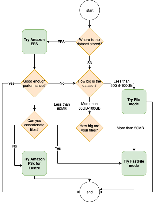
When to use Amazon EFS

If your dataset is primarily stored on Amazon EFS, you may have a preprocessing or annotations application that uses Amazon EFS for storage. You could easily run a training job configured with a data channel that points to the Amazon EFS file system (for more information, refer to Speed up training on Amazon SageMaker using Amazon FSx for Lustre and Amazon EFS file systems). If performance is not quite as good as you expected, check your optimization options with the Amazon EFS performance guide, or consider other input modes.

Use File mode for small datasets

If the dataset is stored on Amazon S3 and its overall volume is relatively small (for example, less than 50–100 GB), try using File mode. The overhead of downloading a dataset of 50 GB can vary based on the total number of files (for example, about 5 minutes if chunked into 100 MB shards). Whether this startup overhead is acceptable primarily depends on the overall duration of your training job, because a longer training phase means a proportionally smaller download phase.

Serializing many small files together

If your dataset size is small (less than 50–100 GB), but is made up of many small files (less than 50 MB), the File mode download overhead grows, because each file needs to be downloaded individually from Amazon S3 to the training instance volume. To reduce this overhead, and to speed up data traversal in general, consider serializing groups of smaller files into fewer larger file containers (such as 150 MB per file) by using file formats such as TFRecord for TensorFlow, WebDataset for PyTorch, or RecordIO for MXNet. These formats require your data loader to iterate through examples sequentially. You could still shuffle your data by randomly reordering the list of TFRecord files after each epoch, and by randomly sampling data from a local shuffle buffer (see the following TensorFlow example).

When to use FastFile mode

For larger datasets with larger files (more than 50 MB), the first option is to try FastFile mode, which is more straightforward to use than FSx for Lustre because it doesn’t require creating a file system, or connecting to a VPC. FastFile mode is ideal for large file containers (more than 150 MB), and might also do well with files more than 50 MB. Because FastFile mode provides a POSIX interface, it supports random reads (reading non-sequential byte-ranges). However, this isn’t the ideal use case, and your throughput would probably be lower than with the sequential reads. However, if you have a relatively large and computationally intensive ML model, FastFile mode may still be able to saturate the effective bandwidth of the training pipeline and not result in an I/O bottleneck. You’ll need to experiment and see. Luckily, switching from File mode to FastFile (and back) is as easy as adding (or removing) the input_mode='FastFile' parameter while defining your input channel using the SageMaker Python SDK:

sagemaker.inputs.TrainingInput(S3_INPUT_FOLDER, input_mode='FastFile') 

No other code or configuration needs to change.

When to use FSx for Lustre

If your dataset is too large for File mode, or has many small files (which you can’t serialize easily), or you have a random read access pattern, FSx for Lustre is a good option to consider. Its file system scales to hundreds of GB/s of throughput and millions of IOPS, which is ideal when you have many small files. However, as already discussed earlier, be mindful of the cold start issues due to lazy loading, and the overhead of setting up and initializing the FSx for Lustre file system.

Cost considerations

For the majority of ML training jobs, especially jobs utilizing GPUs or purpose-built ML chips, most of the cost to train is the ML training instance’s billable seconds. Storage GB per month, API requests, and provisioned throughput are additional costs that are directly associated with the data sources you use.

Storage GB per month

Storage GB per month can be significant for larger datasets, such as videos, LiDAR sensor data, and AdTech real-time bidding logs. For example, storing 1 TB in the Amazon S3 Intelligent-Tiering Frequent Access Tier costs $23 per month. Adding the FSx for Lustre file system on top of Amazon S3 results in additional costs. For example, creating a 1.2 TB file system of SSD-backed Scratch 2 type with data compression disabled costs an additional $168 per month ($140/TB/month).

With Amazon S3 and Amazon EFS, you pay only for what you use, meaning that you’re charged according to the actual dataset size. With FSx for Lustre, you’re charged by the provisioned file system size (1.2 TB at minimum). When running ML instances with EBS volumes, Amazon EBS is charged independently of the ML instance. This is usually a much lower cost compared to the cost of running the instance. For example, running an ml.p3.2xlarge instance with a 100 GB EBS volume for 1 hour costs $3.825 for the instance and $0.02 for the EBS volume.

API requests and provisioned throughput cost

While your training job is crunching through the dataset, it lists and fetches files by dispatching Amazon S3 API requests. For example, each million GET requests is priced at $0.4 (with the Intelligent-Tiering class). You should expect no data transfer cost for bandwidth in and out of Amazon S3, because training takes place in a single Availability Zone.

When using an FSx for Lustre that is linked to an S3 bucket, you incur Amazon S3 API request costs for reading data that isn’t yet cached in the file system, because FSx For Lustre proxies the request to Amazon S3 (and caches the result). There are no direct request costs for FSx for Lustre itself. When you use an FSx for Lustre file system, avoid costs for cross-Availability Zone data transfer by running your training job connected to the same Availability Zone that you provisioned the file system in. Amazon EFS with provisioned throughput adds an extra cost to consdier beyond GB per month.

Performance case study

To demonstrate the training performance considerations mentioned earlier, we performed a series of benchmarks for a realistic use case in the computer vision domain. The benchmark (and takeaways) from this section might not be applicable to all scenarios, and are affected by various predetermined factors we used, such as DNN. We ran tests for 12 combinations of the following:

• Input modes – FSx for Lustre, File mode, FastFile mode
• Dataset size – Smaller dataset (1 GB), larger dataset (54 GB)
• File size – Smaller files (JPGs, approximately 39 KB), Larger files (TFRecord, approximately 110 MB)

For this case study, we chose the most widely used input modes, and therefore omitted Amazon EFS and Pipe mode.

The case study benchmarks were designed as end-to-end SageMaker TensorFlow training jobs on an ml.p3.2xlarge single-GPU instance. We chose the renowned ResNet-50 as our backbone model for the classification task and Caltech-256 as the smaller training dataset (which we replicated 50 times to create its larger dataset version). We performed the training for one epoch, defined as a single full sweep thought the training examples.

The following graphs show the total billable time of the SageMaker training jobs for each benchmark scenario. The total job time itself is comprised of downloading, training, and other stages (such as container startup and uploading trained model artifacts to Amazon S3). Shorter billable times translate into faster and cheaper training jobs.

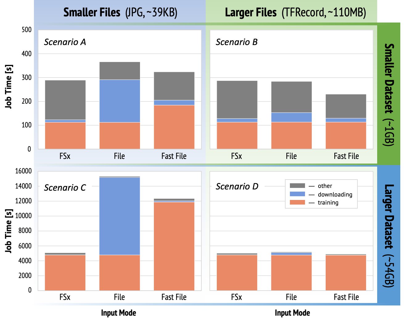
Let’s first discuss Scenario A and Scenario C, which conveniently demonstrate the performance difference between input modes when the dataset is comprised of many small files.

Scenario A (smaller files, smaller dataset) reveals that the training job with the FSx for Lustre file system has the smallest billable time. It has the shortest downloading phase, and its training stage is as fast as File mode, but faster than FastFile. FSx for Lustre is the winner in this single epoch test. Having said that, consider a similar workload but with multiple epochs—the relative overhead of File mode due to the downloading stage decreases as more epochs are added. In this case, we prefer File mode for its ease of use. Additionally, you might find that using File mode and paying for 100 extra billable seconds is a better choice than paying for and provisioning an FSx for Lustre file system.

Scenario C (smaller files, larger dataset) shows FSx for Lustre as the fastest mode, with only 5,000 seconds of total billable time. It also has the shortest downloading stage, because mounting the FSx for Lustre file system doesn’t depend on the number of files in the file system (1.5 million files in this case). The downloading overhead of FastFile is also small; it only fetches metadata of the files residing under the specified S3 bucket prefix, while the content of the files is read during the training stage. File mode is the slowest mode, spending 10,000 seconds to download the entire dataset upfront before starting training. When we look at the training stage, FSx for Lustre and File mode demonstrate similar excellent performance. As for FastFile mode, when streaming smaller files directly from Amazon S3, the overhead for dispatching a new GET request for each file becomes significant relative to the total duration of the file transfer (despite using a highly parallel data loader with prefetch buffer). This results in an overall lower throughput for FastFile mode, which creates an I/O bottleneck for the training job. FSx for Lustre is the clear winner in this scenario.

Scenarios B and D show the performance difference across input modes when the dataset is comprised of fewer larger files. Reading sequentially using larger files typically results in better I/O performance because it allows effective buffering and reduces the number of I/O operations.

Scenario B (larger files, smaller dataset) shows similar training stage time for all modes (testifying that the training isn’t I/O-bound). In this scenario, we prefer FastFile mode over File mode due to shorter downloading stage, and prefer FastFile mode over FSx for Lustre due to the ease of use of the former.

Scenario D (larger files, larger dataset) shows relatively similar total billable times for all three modes. The downloading phase of File mode is longer than that of FSx for Lustre and FastFile. File mode downloads the entire dataset (54 GB) from Amazon S3 to the training instance before starting the training stage. All three modes spend similar time in the training phase, because all modes can fetch data fast enough and are GPU-bound. If we use ML instances with additional CPU or GPU resources, such as ml.p4d.24xlarge, the required data I/O throughput to saturate the compute resources grows. In these cases, we can expect FastFile and FSx for Lustre to successfully scale their throughput (however, FSx for Lustre throughput depends on provisioned file system size). The ability of File mode to scale its throughput depends on the throughput of the disk volume attached to the instance. For example, Amazon EBS-backed instances (like ml.p3.2xlarge, ml.p3.8xlarge, and ml.p3.16xlarge) are limited to a maximum throughput of 250MB/s, whereas local NVMe-backed instances (like ml.g5.* or ml.p4d.24xlarge) can accommodate a much larger throughput.

To summarize, we believe FastFile is the winner for this scenario because it’s faster than File mode, and just as fast as FSx for Lustre, yet more straightforward to use, costs less, and can easily scale up its throughput as needed.

Additionally, if we had a much larger dataset (several TBs in size), File mode would spend many hours downloading the dataset before training could start, whereas FastFile could start training significantly more quickly.

Bring your own data ingestion

The native data source of SageMaker fits most but not all possible ML training scenarios. The situations when you might need to look for other data ingestion options could include reading data directly from a third-party storage product (assuming an easy and timely export to Amazon S3 isn’t possible), or having a strong requirement for the same training script to run unchanged on both SageMaker and Amazon Elastic Compute Cloud (Amazon EC2) or Amazon Elastic Kubernetes Service (Amazon EKS). You can address these cases by implementing your data ingestion mechanism into the training script. This mechanism is responsible for reading datasets from external data sources into the training instance. For example, the TFRecordDataset of the TensorFlow’s tf.data library can read directly from Amazon S3 storage.

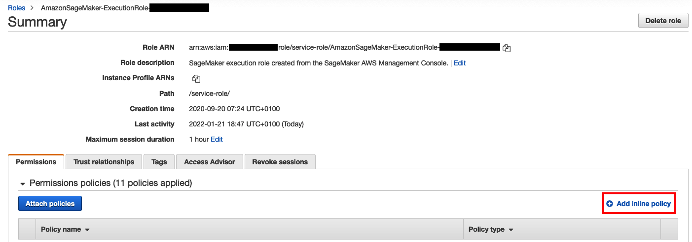
If your data ingestion mechanism needs to call any AWS services, such as Amazon Relational Database Service (Amazon RDS), make sure that the AWS Identity and Access Management (IAM) role of your training job includes the relevant IAM policies. If the data source resides in Amazon Virtual Private Cloud (Amazon VPC), you need to run your training job connected to the same VPC.

When you’re managing dataset ingestion yourself, SageMaker lineage tracking can’t automatically log the datasets used during training. Therefore, consider alternative mechanisms, like training job tags or hyperparameters, to capture your relevant metadata.

Conclusion

Choosing the right SageMaker training data source could have a profound effect on the speed, ease of use, and cost of training ML models. Use the provided flowchart to get started quickly, observe the results, and experiment with additional configuration as needed. Keep in mind the pros, cons, and limitations of each data source, and how well they suit your training job’s individual requirements. Reach out to an AWS contact for further information and assistance.

About the Authors

Gili Nachum is a senior AI/ML Specialist Solutions Architect who works as part of the EMEA Amazon Machine Learning team. Gili is passionate about the challenges of training deep learning models, and how machine learning is changing the world as we know it. In his spare time, Gili enjoy playing table tennis.

Dr. Alexander Arzhanov is an AI/ML Specialist Solutions Architect based in Frankfurt, Germany. He helps AWS customers to design and deploy their ML solutions across EMEA region. Prior to joining AWS, Alexander was researching origins of heavy elements in our universe and grew passionate about ML after using it in his large-scale scientific calculations.

Read More

This is a guest post authored by Dr. Janhavi Punyarthi, Director of Brand Development at InpharmD.

The intersection of DI and AI: Drug information (DI) refers to the discovery, use, and management of healthcare and medical information. Healthcare providers have many challenges associated with drug information discovery, such as intensive time involvement, lack of accessibility, and accuracy of reliable data. The average clinical query requires a literature search that takes an average of 18.5 hours. In addition, drug information often lies in disparate information silos, behind pay walls and design walls, and quickly becomes stale.

InpharmD is a mobile-based, academic network of drug information centers that combines the power of artificial intelligence and pharmacy intelligence to provide curated, evidence-based responses to clinical inquiries. The goal at InpharmD is to deliver accurate drug information efficiently, so healthcare providers can make informed decisions quickly and provide optimal patient care.

To meet this goal, InpharmD built Sherlock, a prototype bot that reads and deciphers medical literature. Sherlock is based on AI services including Amazon Kendra, an intelligent search service, and Amazon Lex, a fully managed AI service for building conversational interfaces into any application. With Sherlock, healthcare providers can retrieve valuable clinical evidence, which allows them to make data-driven decisions and spend more time with patients. Sherlock has access to over 5,000 of InpharmD’s abstracts and 1,300 drug monographs from the American Society of Health System Pharmacists (ASHP). This data bank expands every day as more abstracts and monographs are uploaded and edited. Sherlock filters for relevancy and recency to quickly search through thousands of PDFs, studies, abstracts, and other documents, and provide responses with 94% accuracy when compared to humans.

The following is a preliminary textual similarity score and manual evaluation between a machine-generated summary and human summary.

InpharmD and AWS

AWS serves as an accelerator for InpharmD. AWS SDKs significantly reduce development time by providing common functionalities that allow InpharmD to focus on delivering quality results. AWS services like Amazon Kendra and Amazon Lex allow InpharmD to worry less about scaling, systems maintenance, and stability.

The following diagram illustrates the architecture of AWS services for Sherlock:

InpharmD would not have been able to build Sherlock without the help of AWS. At the core, InpharmD uses Amazon Kendra as the foundation of its machine learning (ML) initiatives to index InpharmD’s library of documents and provide smart answers using natural language processing. This is superior to traditional fuzzy search-based algorithms, and the result is better answers for user questions.

InpharmD then used Amazon Lex to create Sherlock, a chatbot service that delivers Amazon Kendra’s ML-powered search results through an easy-to-use conversational interface. Sherlock uses the natural language understanding capabilities of Amazon Lex to detect the intent and better understand the context of questions in order to find the best answers. This allows for more natural conversations regarding medical literature inquiries and responses.

In addition, InpharmD stores the drug information content in the cloud via S3 buckets. AWS Lambda allows InpharmD to scale server logic and interact with various AWS services with ease. It is key in connecting Amazon Kendra to other services such as Amazon Lex.

“AWS has been essential in accelerating the development of Sherlock. We don’t have to worry as much about scaling, systems maintenance, and stability because AWS takes care of it for us. With Amazon Kendra and Amazon Lex, we’re able to build the best version of Sherlock and reduce our development time by months. On top of that, we’re also able to decrease the time for each literature search by 16%.”

– Tulasee Chintha, Chief Technological Officer and co-founder of InpharmD.

Impact

Trusted by a network of over 10,000 providers and eight health systems, InpharmD helps guide evidence-based information that accelerates decision-making and saves time for clinicians. With the help of InpharmD services, the time for each literature search is decreased by 16%, saving approximately 3 hours per search. InpharmD also provides a comprehensive result, with approximately 12 journal articles summaries for each literature search. With the implementation of Sherlock, InpharmD hopes to make the literature search process even more efficient, summarizing more studies in less time.

The Sherlock prototype is currently being beta tested and shared with providers to get user feedback.

“Access to the InpharmD platform is very customizable. I was happy that the InpharmD team worked with me to meet my specific needs and the needs of my institution. I asked Sherlock about the safety of a drug and the product gave me a summary and literature to answer complex clinical questions fast. This product does a lot of the work that earlier involved a lot of clicking and searching and trying tons of different search vendors. For a busy physician, it works great. It saved me time and helped ensure I was using the most up-to-date research for my decision-making. This would’ve been a game changer when I was at an academic hospital doing clinical research, but even as a private physician it’s great to ensure you’re always up to date with the current evidence.”

– Ghaith Ibrahim, MD at Wellstar Health System.

Conclusion

Our team at InpharmD is excited to build on the early success we have seen from deploying Sherlock with the help of Amazon Kendra and Amazon Lex. Our plan for Sherlock is to evolve it into an intelligent assistant that is available anytime, anywhere. In the future, we hope to integrate Sherlock with Amazon Alexa so providers can have immediate, contactless access to evidence, allowing them to make fast data-driven clinical decisions that ensure optimal patient care.

About the Author

Dr. Janhavi Punyarthi is an innovative pharmacist leading brand development and engagement at InpharmD. With a passion for creativity, Dr. Punyarthi enjoys combining her love for writing and evidence-based medicine to present clinical literature in engaging ways.

Disclaimer: AWS is not responsible for the content or accuracy of this post. The content and opinions in this post are solely those of the third-party author. It is each customers’ responsibility to determine whether they are subject to HIPAA, and if so, how best to comply with HIPAA and its implementing regulations. Before using AWS in connection with protected health information, customers must enter an AWS Business Associate Addendum (BAA) and follow its configuration requirements.

Read More