Amazon SageMaker Inference has been a popular tool for deploying advanced machine learning (ML) and generative AI models at scale. As AI applications become increasingly complex, customers want to deploy multiple models in a coordinated group that collectively process inference requests for an application. In addition, with the evolution of generative AI applications, many use cases now require inference workflows—sequences of interconnected models operating in predefined logical flows. This trend drives a growing need for more sophisticated inference offerings.
To address this need, we are introducing a new capability in the SageMaker Python SDK that revolutionizes how you build and deploy inference workflows on SageMaker. We will take Amazon Search as an example to show case how this feature is used in helping customers building inference workflows. This new Python SDK capability provides a streamlined and simplified experience that abstracts away the underlying complexities of packaging and deploying groups of models and their collective inference logic, allowing you to focus on what matter most—your business logic and model integrations.
In this post, we provide an overview of the user experience, detailing how to set up and deploy these workflows with multiple models using the SageMaker Python SDK. We walk through examples of building complex inference workflows, deploying them to SageMaker endpoints, and invoking them for real-time inference. We also show how customers like Amazon Search plan to use SageMaker Inference workflows to provide more relevant search results to Amazon shoppers.
Whether you are building a simple two-step process or a complex, multimodal AI application, this new feature provides the tools you need to bring your vision to life. This tool aims to make it easy for developers and businesses to create and manage complex AI systems, helping them build more powerful and efficient AI applications.
In the following sections, we dive deeper into details of the SageMaker Python SDK, walk through practical examples, and showcase how this new capability can transform your AI development and deployment process.
Key improvements and user experience
The SageMaker Python SDK now includes new features for creating and managing inference workflows. These additions aim to address common challenges in developing and deploying inference workflows:
- Deployment of multiple models – The core of this new experience is the deployment of multiple models as inference components within a single SageMaker endpoint. With this approach, you can create a more unified inference workflow. By consolidating multiple models into one endpoint, you can reduce the number of endpoints that need to be managed. This consolidation can also improve operational tasks, resource utilization, and potentially costs.
- Workflow definition with workflow mode – The new workflow mode extends the existing Model Builder capabilities. It allows for the definition of inference workflows using Python code. Users familiar with the
ModelBuilderclass might find this feature to be an extension of their existing knowledge. This mode enables creating multi-step workflows, connecting models, and specifying the data flow between different models in the workflows. The goal is to reduce the complexity of managing these workflows and enable you to focus more on the logic of the resulting compound AI system. - Development and deployment options – A new deployment option has been introduced for the development phase. This feature is designed to allow for quicker deployment of workflows to development environments. The intention is to enable faster testing and refinement of workflows. This could be particularly relevant when experimenting with different configurations or adjusting models.
- Invocation flexibility – The SDK now provides options for invoking individual models or entire workflows. You can choose to call a specific inference component used in a workflow or the entire workflow. This flexibility can be useful in scenarios where access to a specific model is needed, or when only a portion of the workflow needs to be executed.
- Dependency management – You can use SageMaker Deep Learning Containers (DLCs) or the SageMaker distribution that comes preconfigured with various model serving libraries and tools. These are intended to serve as a starting point for common use cases.
To get started, use the SageMaker Python SDK to deploy your models as inference components. Then, use the workflow mode to create an inference workflow, represented as Python code using the container of your choice. Deploy the workflow container as another inference component on the same endpoints as the models or a dedicated endpoint. You can run the workflow by invoking the inference component that represents the workflow. The user experience is entirely code-based, using the SageMaker Python SDK. This approach allows you to define, deploy, and manage inference workflows using SDK abstractions offered by this feature and Python programming. The workflow mode provides flexibility to specify complex sequences of model invocations and data transformations, and the option to deploy as components or endpoints caters to various scaling and integration needs.
Solution overview
The following diagram illustrates a reference architecture using the SageMaker Python SDK.

The improved SageMaker Python SDK introduces a more intuitive and flexible approach to building and deploying AI inference workflows. Let’s explore the key components and classes that make up the experience:
ModelBuildersimplifies the process of packaging individual models as inference components. It handles model loading, dependency management, and container configuration automatically.- The
CustomOrchestratorclass provides a standardized way to define custom inference logic that orchestrates multiple models in the workflow. Users implement thehandle()method to specify this logic and can use an orchestration library or none at all (plain Python). - A single
deploy()call handles the deployment of the components and workflow orchestrator. - The Python SDK supports invocation against the custom inference workflow or individual inference components.
- The Python SDK supports both synchronous and streaming inference.
CustomOrchestrator is an abstract base class that serves as a template for defining custom inference orchestration logic. It standardizes the structure of entry point-based inference scripts, making it straightforward for users to create consistent and reusable code. The handle method in the class is an abstract method that users implement to define their custom orchestration logic.
With this templated class, users can integrate into their custom workflow code, and then point to this code in the model builder using a file path or directly using a class or method name. Using this class and the ModelBuilder class, it enables a more streamlined workflow for AI inference:
- Users define their custom workflow by implementing the
CustomOrchestratorclass. - The custom
CustomOrchestratoris passed toModelBuilderusing theModelBuilder inference_specparameter. ModelBuilderpackages theCustomOrchestratoralong with the model artifacts.- The packaged model is deployed to a SageMaker endpoint (for example, using a TorchServe container).
- When invoked, the SageMaker endpoint uses the custom handle() function defined in the
CustomOrchestratorto handle the input payload.
In the follow sections, we provide two examples of custom workflow orchestrators implemented with plain Python code. For simplicity, the examples use two inference components.
We explore how to create a simple workflow that deploys two large language models (LLMs) on SageMaker Inference endpoints along with a simple Python orchestrator that calls the two models. We create an IT customer service workflow where one model processes the initial request and another suggests solutions. You can find the example notebook in the GitHub repo.
Prerequisites
To run the example notebooks, you need an AWS account with an AWS Identity and Access Management (IAM) role with least-privilege permissions to manage resources created. For details, refer to Create an AWS account. You might need to request a service quota increase for the corresponding SageMaker hosting instances. In this example, we host multiple models on the same SageMaker endpoint, so we use two ml.g5.24xlarge SageMaker hosting instances.
Python inference orchestration
First, let’s define our custom orchestration class that inherits from CustomOrchestrator. The workflow is structured around a custom inference entry point that handles the request data, processes it, and retrieves predictions from the configured model endpoints. See the following code:
This code performs the following functions:
- Defines the orchestration that sequentially calls two models using their inference component names
- Processes the response from the first model before passing it to the second model
- Returns the final generated response
This plain Python approach provides flexibility and control over the request-response flow, enabling seamless cascading of outputs across multiple model components.
Build and deploy the workflow
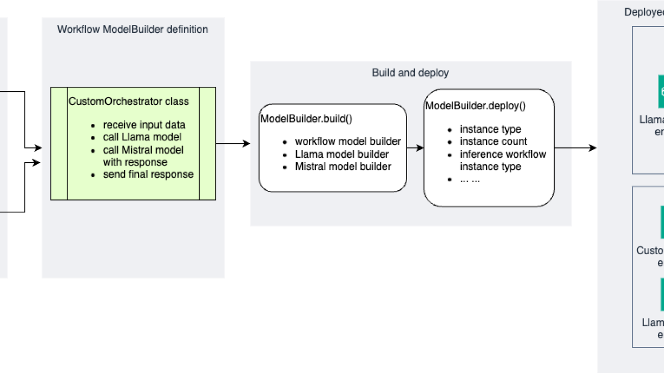
To deploy the workflow, we first create our inference components and then build the custom workflow. One inference component will host a Meta Llama 3.1 8B model, and the other will host a Mistral 7B model.
Now we can tie it all together to create one more ModelBuilder to which we pass the modelbuilder_list, which contains the ModelBuilder objects we just created for each inference component and the custom workflow. Then we call the build() function to prepare the workflow for deployment.
In the preceding code snippet, you can comment out the section that defines the resource_requirements to have the custom workflow deployed on a separate endpoint instance, which can be a dedicated CPU instance to handle the custom workflow payload.
By calling the deploy() function, we deploy the custom workflow and the inference components to your desired instance type, in this example ml.g5.24.xlarge. If you choose to deploy the custom workflow to a separate instance, by default, it will use the ml.c5.xlarge instance type. You can set inference_workflow_instance_type and inference_workflow_initial_instance_count to configure the instances required to host the custom workflow.
Invoke the endpoint
After you deploy the workflow, you can invoke the endpoint using the predictor object:
You can also invoke each inference component in the deployed endpoint. For example, we can test the Llama inference component with a synchronous invocation, and Mistral with streaming:
When handling the streaming response, we need to read each line of the output separately. The following example code demonstrates this streaming handling by checking for newline characters to separate and print each token in real time:
So far, we have walked through the example code to demonstrate how to build complex inference logic using Python orchestration, deploy them to SageMaker endpoints, and invoke them for real-time inference. The Python SDK automatically handles the following:
- Model packaging and container configuration
- Dependency management and environment setup
- Endpoint creation and component coordination
Whether you’re building a simple workflow of two models or a complex multimodal application, the new SDK provides the building blocks needed to bring your inference workflows to life with minimal boilerplate code.
Customer story: Amazon Search
Amazon Search is a critical component of the Amazon shopping experience, processing an enormous volume of queries across billions of products across diverse categories. At the core of this system are sophisticated matching and ranking workflows, which determine the order and relevance of search results presented to customers. These workflows execute large deep learning models in predefined sequences, often sharing models across different workflows to improve price-performance and accuracy. This approach makes sure that whether a customer is searching for electronics, fashion items, books, or other products, they receive the most pertinent results tailored to their query.
The SageMaker Python SDK enhancement offers valuable capabilities that align well with Amazon Search’s requirements for these ranking workflows. It provides a standard interface for developing and deploying complex inference workflows crucial for effective search result ranking. The enhanced Python SDK enables efficient reuse of shared models across multiple ranking workflows while maintaining the flexibility to customize logic for specific product categories. Importantly, it allows individual models within these workflows to scale independently, providing optimal resource allocation and performance based on varying demand across different parts of the search system.
Amazon Search is exploring the broad adoption of these Python SDK enhancements across their search ranking infrastructure. This initiative aims to further refine and improve search capabilities, enabling the team to build, version, and catalog workflows that power search ranking more effectively across different product categories. The ability to share models across workflows and scale them independently offers new levels of efficiency and adaptability in managing the complex search ecosystem.
Vaclav Petricek, Sr. Manager of Applied Science at Amazon Search, highlighted the potential impact of these SageMaker Python SDK enhancements: “These capabilities represent a significant advancement in our ability to develop and deploy sophisticated inference workflows that power search matching and ranking. The flexibility to build workflows using Python, share models across workflows, and scale them independently is particularly exciting, as it opens up new possibilities for optimizing our search infrastructure and rapidly iterating on our matching and ranking algorithms as well as new AI features. Ultimately, these SageMaker Inference enhancements will allow us to more efficiently create and manage the complex algorithms powering Amazon’s search experience, enabling us to deliver even more relevant results to our customers.”
The following diagram illustrates a sample solution architecture used by Amazon Search.

Clean up
When you’re done testing the models, as a best practice, delete the endpoint to save costs if the endpoint is no longer required. You can follow the cleanup section the demo notebook or use following code to delete the model and endpoint created by the demo:
Conclusion
The new SageMaker Python SDK enhancements for inference workflows mark a significant advancement in the development and deployment of complex AI inference workflows. By abstracting the underlying complexities, these enhancements empower inference customers to focus on innovation rather than infrastructure management. This feature bridges sophisticated AI applications with the robust SageMaker infrastructure, enabling developers to use familiar Python-based tools while harnessing the powerful inference capabilities of SageMaker.
Early adopters, including Amazon Search, are already exploring how these capabilities can drive major improvements in AI-powered customer experiences across diverse industries. We invite all SageMaker users to explore this new functionality, whether you’re developing classic ML models, building generative AI applications or multi-model workflows, or tackling multi-step inference scenarios. The enhanced SDK provides the flexibility, ease of use, and scalability needed to bring your ideas to life. As AI continues to evolve, SageMaker Inference evolves with it, providing you with the tools to stay at the forefront of innovation. Start building your next-generation AI inference workflows today with the enhanced SageMaker Python SDK.
About the authors
 Melanie Li, PhD, is a Senior Generative AI Specialist Solutions Architect at AWS based in Sydney, Australia, where her focus is on working with customers to build solutions leveraging state-of-the-art AI and machine learning tools. She has been actively involved in multiple Generative AI initiatives across APJ, harnessing the power of Large Language Models (LLMs). Prior to joining AWS, Dr. Li held data science roles in the financial and retail industries.
 Saurabh Trikande is a Senior Product Manager for Amazon Bedrock and SageMaker Inference. He is passionate about working with customers and partners, motivated by the goal of democratizing AI. He focuses on core challenges related to deploying complex AI applications, inference with multi-tenant models, cost optimizations, and making the deployment of Generative AI models more accessible. In his spare time, Saurabh enjoys hiking, learning about innovative technologies, following TechCrunch, and spending time with his family.
 Osho Gupta is a Senior Software Developer at AWS SageMaker. He is passionate about ML infrastructure space, and is motivated to learn & advance underlying technologies that optimize Gen AI training & inference performance. In his spare time, Osho enjoys paddle boarding, hiking, traveling, and spending time with his friends & family.
 Joseph Zhang is a software engineer at AWS. He started his AWS career at EC2 before eventually transitioning to SageMaker, and now works on developing GenAI-related features. Outside of work he enjoys both playing and watching sports (go Warriors!), spending time with family, and making coffee.
 Gary Wang is a Software Developer at AWS SageMaker. He is passionate about AI/ML operations and building new things. In his spare time, Gary enjoys running, hiking, trying new food, and spending time with his friends and family.
 James Park is a Solutions Architect at Amazon Web Services. He works with Amazon.com to design, build, and deploy technology solutions on AWS, and has a particular interest in AI and machine learning. In h is spare time he enjoys seeking out new cultures, new experiences, and staying up to date with the latest technology trends. You can find him on LinkedIn.
 Vaclav Petricek is a Senior Applied Science Manager at Amazon Search, where he led teams that built Amazon Rufus and now leads science and engineering teams that work on the next generation of Natural Language Shopping. He is passionate about shipping AI experiences that make people’s lives better. Vaclav loves off-piste skiing, playing tennis, and backpacking with his wife and three children.
 Wei Li is a Senior Software Dev Engineer in Amazon Search. She is passionate about Large Language Model training and inference technologies, and loves integrating these solutions into Search Infrastructure to enhance natural language shopping experiences. During her leisure time, she enjoys gardening, painting, and reading.
 Brian Granger is a Senior Principal Technologist at Amazon Web Services and a professor of physics and data science at Cal Poly State University in San Luis Obispo, CA. He works at the intersection of UX design and engineering on tools for scientific computing, data science, machine learning, and data visualization. Brian is a co-founder and leader of Project Jupyter, co-founder of the Altair project for statistical visualization, and creator of the PyZMQ project for ZMQ-based message passing in Python. At AWS he is a technical and open source leader in the AI/ML organization. Brian also represents AWS as a board member of the PyTorch Foundation. He is a winner of the 2017 ACM Software System Award and the 2023 NASA Exceptional Public Achievement Medal for his work on Project Jupyter. He has a Ph.D. in theoretical physics from the University of Colorado.


 Amit Chaudhary Amit Chaudhary is a Senior Solutions Architect at Amazon Web Services. His focus area is AI/ML, and he helps customers with generative AI, large language models, and prompt engineering. Outside of work, Amit enjoys spending time with his family.
 Nikhil Jha Nikhil Jha is a Senior Technical Account Manager at Amazon Web Services. His focus areas include AI/ML, building Generative AI resources, and analytics. In his spare time, he enjoys exploring the outdoors with his family.
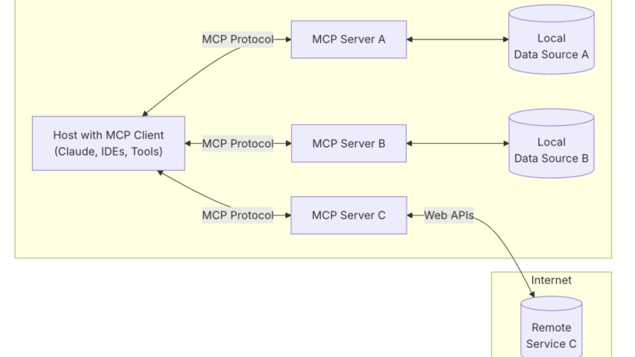


 Joel Asante, an Austin-based Solutions Architect at Amazon Web Services (AWS), works with GovTech (Government Technology) customers. With a strong background in data science and application development, he brings deep technical expertise to creating secure and scalable cloud architectures for his customers. Joel is passionate about data analytics, machine learning, and robotics, leveraging his development experience to design innovative solutions that meet complex government requirements. He holds 13 AWS certifications and enjoys family time, fitness, and cheering for the Kansas City Chiefs and Los Angeles Lakers in his spare time.
 Dunieski Otano is a Solutions Architect at Amazon Web Services based out of Miami, Florida. He works with World Wide Public Sector MNO (Multi-International Organizations) customers. His passion is Security, Machine Learning and Artificial Intelligence, and Serverless. He works with his customers to help them build and deploy high available, scalable, and secure solutions. Dunieski holds 14 AWS certifications and is an AWS Golden Jacket recipient. In his free time, you will find him spending time with his family and dog, watching a great movie, coding, or flying his drone.
 Varun Jasti is a Solutions Architect at Amazon Web Services, working with AWS Partners to design and scale artificial intelligence solutions for public sector use cases to meet compliance standards. With a background in Computer Science, his work covers broad range of ML use cases primarily focusing on LLM training/inferencing and computer vision. In his spare time, he loves playing tennis and swimming.
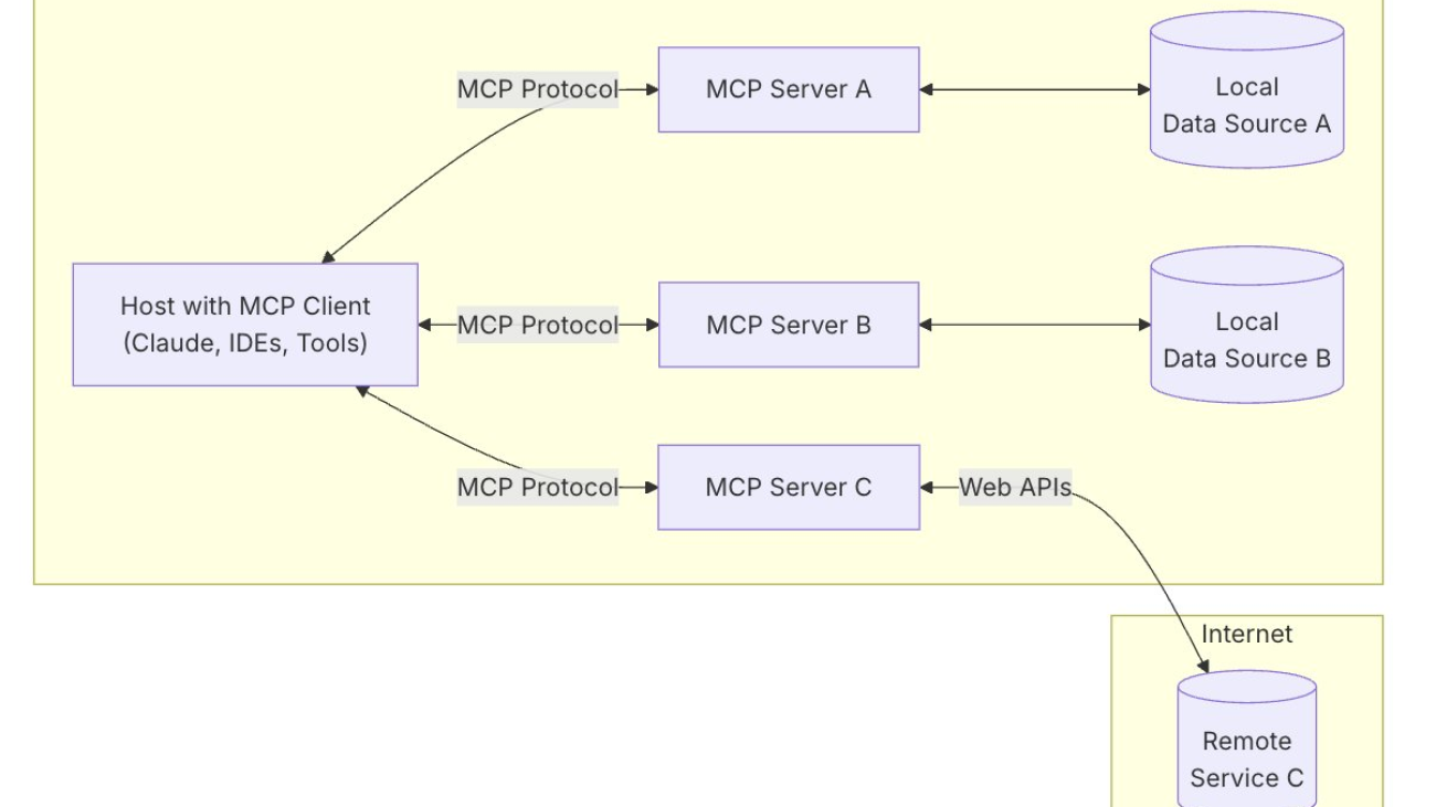


 Koushik Kethamakka is a Senior Software Engineer at AWS, focusing on AI/ML initiatives. At Amazon, he led real-time ML fraud prevention systems for Amazon.com before moving to AWS to lead development of AI/ML services like Amazon Lex and Amazon Bedrock. His expertise spans product and system design, LLM hosting, evaluations, and fine-tuning. Recently, Koushik’s focus has been on LLM evaluations and safety, leading to the development of products like Amazon Bedrock Evaluations and Amazon Bedrock Guardrails. Prior to joining Amazon, Koushik earned his MS from the University of Houston.
 Hang Su is a Senior Applied Scientist at AWS AI. He has been leading the Amazon Bedrock Guardrails Science team. His interest lies in AI safety topics, including harmful content detection, red-teaming, sensitive information detection, among others.
 Shyam Srinivasan is on the Amazon Bedrock product team. He cares about making the world a better place through technology and loves being part of this journey. In his spare time, Shyam likes to run long distances, travel around the world, and experience new cultures with family and friends.
 Aartika Sardana Chandras is a Senior Product Marketing Manager for AWS Generative AI solutions, with a focus on Amazon Bedrock. She brings over 15 years of experience in product marketing, and is dedicated to empowering customers to navigate the complexities of the AI lifecycle. Aartika is passionate about helping customers leverage powerful AI technologies in an ethical and impactful manner.
 Satveer Khurpa is a Sr. WW Specialist Solutions Architect, Amazon Bedrock at Amazon Web Services, specializing in Amazon Bedrock security. In this role, he uses his expertise in cloud-based architectures to develop innovative generative AI solutions for clients across diverse industries. Satveer’s deep understanding of generative AI technologies and security principles allows him to design scalable, secure, and responsible applications that unlock new business opportunities and drive tangible value while maintaining robust security postures.
 Antonio Rodriguez is a Principal Generative AI Specialist Solutions Architect at Amazon Web Services. He helps companies of all sizes solve their challenges, embrace innovation, and create new business opportunities with Amazon Bedrock. Apart from work, he loves to spend time with his family and play sports with his friends.


 Adam Nemeth is a Senior Solutions Architect at AWS, where he helps global financial customers embrace cloud computing through architectural guidance and technical support. With over 24 years of IT expertise, Adam previously worked at UBS before joining AWS. He lives in Switzerland with his wife and their three children.
 Dominic Searle is a Senior Solutions Architect at Amazon Web Services, where he has had the pleasure of working with Global Financial Services customers as they explore how Generative AI can be integrated into their technology strategies. Providing technical guidance, he enjoys helping customers effectively leverage AWS Services to solve real business problems.
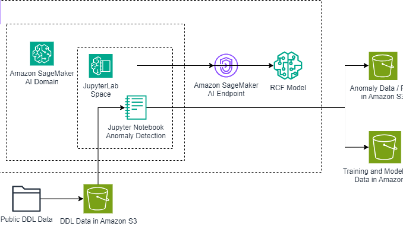


 Dr. Ian Lunsford is an Aerospace AI Engineer at AWS Professional Services. He integrates cloud services into aerospace applications. Additionally, Ian focuses on building AI/ML solutions using AWS services.
 Nick Biso is a Machine Learning Engineer at AWS Professional Services. He solves complex organizational and technical challenges using data science and engineering. In addition, he builds and deploys AI/ML models on the AWS Cloud. His passion extends to his proclivity for travel and diverse cultural experiences.


 Justin Ossai is a GenAI Labs Specialist Solutions Architect based in Dallas, TX. He is a highly passionate IT professional with over 15 years of technology experience. He has designed and implemented solutions with on-premises and cloud-based infrastructure for small and enterprise companies.
 Michael Hsieh is a Principal AI/ML Specialist Solutions Architect. He works with HCLS customers to advance their ML journey with AWS technologies and his expertise in medical imaging. As a Seattle transplant, he loves exploring the great mother nature the city has to offer, such as the hiking trails, scenery kayaking in the SLU, and the sunset at Shilshole Bay.
 Shreya Mohanty is a Deep Learning Architect at the AWS Generative AI Innovation Center, where she partners with customers across industries to design and implement high-impact GenAI-powered solutions. She specializes in translating customer goals into tangible outcomes that drive measurable impact.
 Rachel Hanspal is a Deep Learning Architect at AWS Generative AI Innovation Center, specializing in end-to-end GenAI solutions with a focus on frontend architecture and LLM integration. She excels in translating complex business requirements into innovative applications, leveraging expertise in natural language processing, automated visualization, and secure cloud architectures.


 Aitzaz Ahmad is an Applied Science Manager at Amazon, where he leads a team of scientists building various applications of machine learning and generative AI in finance. His research interests are in natural language processing (NLP), generative AI, and LLM agents. He received his PhD in electrical engineering from Texas A&M University.
 Stephen Lau is a Senior Manager of Software Development at Amazon, leads teams of scientists and engineers. His team develops powerful fraud detection and prevention applications, saving Amazon billions annually. They also build Treasury applications that optimize Amazon global liquidity while managing risks, significantly impacting the financial security and efficiency of Amazon.
 Yong Xie is an applied scientist in Amazon FinTech. He focuses on developing large language models and generative AI applications for finance.
 Kristen Henkels is a Sr. Product Manager – Technical in Amazon FinTech, where she focuses on helping internal teams improve their productivity by leveraging ML and AI solutions. She holds an MBA from Columbia Business School and is passionate about empowering teams with the right technology to enable strategic, high-value work.
 Shivansh Singh is a Principal Solutions Architect at Amazon. He is passionate about driving business outcomes through innovative, cost-effective and resilient solutions, with a focus on machine learning, generative AI, and serverless technologies. He is a technical leader and strategic advisor to large-scale games, media, and entertainment customers. He has over 16 years of experience transforming businesses through technological innovations and building large-scale enterprise solutions.
 Dushan Tharmal is a Principal Product Manager – Technical on the Amazons Artificial General Intelligence team, responsible for the Amazon Nova Foundation Models. He earned his bachelor’s in mathematics at the University of Waterloo and has over 10 years of technical product leadership experience across financial services and loyalty. In his spare time, he enjoys wine, hikes, and philosophy.
 Anupam Dewan is a Senior Solutions Architect with a passion for generative AI and its applications in real life. He and his team enable Amazon builders who build customer-facing applications using generative AI. He lives in the Seattle area, and outside of work, he loves to go hiking and enjoy nature.