Businesses often face challenges in managing and deriving value from their data. According to McKinsey, 78% of organizations now use AI in at least one business function (as of 2024), showing the growing importance of AI solutions in business. Additionally, 21% of organizations using generative AI have fundamentally redesigned their workflows, showing how AI is transforming business operations.
Gartner identifies AI-powered analytics and reporting as a core investment area for retail organizations, with most large retailers expected to deploy or scale such solutions within the next 12–18 months. The retail sector’s data complexity demands sophisticated solutions that can integrate seamlessly with existing systems. Amazon Q Business offers features that can be tailored to meet specific business needs, including integration capabilities with popular retail management systems, point-of-sale systems, inventory management software, and ecommerce systems. Through advanced AI algorithms, the system analyzes historical data and current trends, helping businesses prepare effectively for seasonal fluctuations in demand and make data-driven decisions.
Amazon Q Business for Retail Intelligence is an AI-powered assistant designed to help retail businesses streamline operations, improve customer service, and enhance decision-making processes. This solution is specifically engineered to be scalable and adaptable to businesses of various sizes, helping them compete more effectively. In this post, we show how you can use Amazon Q Business for Retail Intelligence to transform your data into actionable insights.
Solution overview
Amazon Q Business for Retail Intelligence is a comprehensive solution that transforms how retailers interact with their data using generative AI. The solution architecture combines the powerful generative AI capabilities of Amazon Q Business and Amazon QuickSight visualizations to deliver actionable insights across the entire retail value chain. Our solution also uses Amazon Q Apps so retail personas and users can create custom AI-powered applications to streamline day-to-day tasks and automate workflows and business processes.
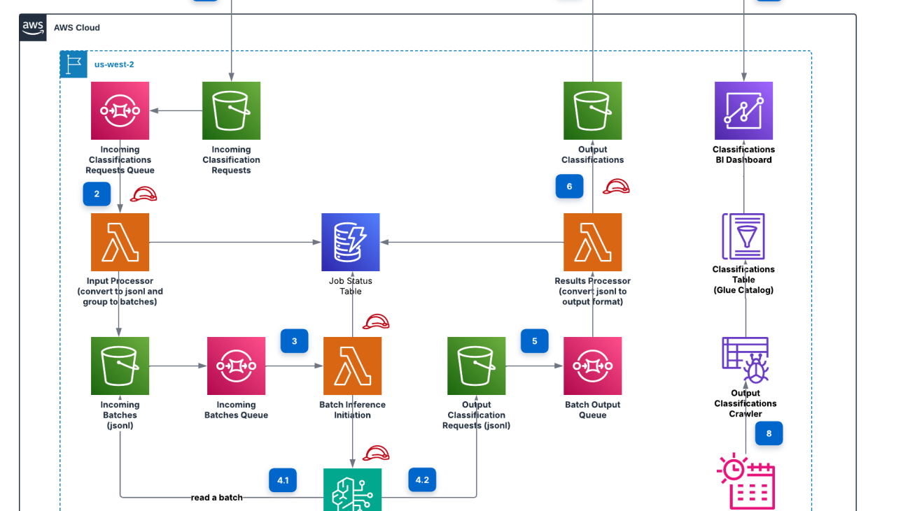
The following diagram illustrates the solution architecture.

The solution uses the AWS architecture above to deliver a secure, high-performance, and reliable solution for retail intelligence. Amazon Q Business serves as the primary generative AI engine, enabling natural language interactions and powering custom retail-specific applications. The architecture incorporates AWS IAM Identity Center for robust authentication and access control, and Amazon Simple Storage Service (Amazon S3) provides secure data lake storage for retail data sources. We use QuickSight for interactive visualizations, enhancing data interpretation. The solution’s flexibility is further enhanced by AWS Lambda for serverless processing, Amazon API Gateway for efficient endpoint management, and Amazon CloudFront for optimized content delivery. This solution uses the Amazon Q Business custom plugin to call the API endpoints to start the automated workflows directly from the Amazon Q Business web application interface based on customer queries and interactions.
This setup implements a three-tier architecture: a data integration layer that securely ingests data from multiple retail sources, a processing layer where Amazon Q Business analyzes queries and generates insights, and a presentation layer that delivers personalized, role-based insights through a unified interface.
We have provided an AWS CloudFormation template, sample datasets, and scripts that you can use to set up the environment for this demonstration.
In the following sections, we dive deeper on how this solution works.
Deployment
We have provided the Amazon Q Business for Retail Intelligence solution as open source—you can use it as a starting point for your own solution and help us make it better by contributing fixes and features through GitHub pull requests. Visit the GitHub repository to explore the code, choose Watch to be notified of new releases, and check the README for the latest documentation updates.
After you set up the environment, you can access the Amazon Q Business for Retail Intelligence dashboard, as shown in the following screenshot.

You can interact with the QuickSight visualizations and Amazon Q Business chat interface to ask questions using natural language.
Key features and capabilities
Retail users can interact with this solution in many ways. In this section, we explore the key features.
For C-suite executives or senior leadership wanting to know how your business is performing, our solution provides a single pane of glass and makes it straightforward to access and interact with your enterprise’s qualitative and quantitative data using natural language. For example, users can analyze quantitative data like product sales or marketing campaign performance using the interactive visualizations powered by QuickSight and qualitative data like customer feedback from Amazon Q Business using natural language, all from a single interface.

Consider that you are a marketing analyst and you want to evaluate campaign performance and reach across channels and conduct an analysis on ad spend vs. revenue. With Amazon Q Business, you can run complex queries with natural language questions and with share the Q Apps with multiple teams. The solution provides automated insights about customer behavior and campaign effectiveness, helping marketing teams make faster decisions and quick adjustments to maximize ROI.

Similarly, let’s assume you are a merchandising planner or a vendor manager and you want to understand the impact of cost-prohibitive events for your international business that deals with importing and exporting of goods and services. You can add inputs to Amazon Q Apps and get responses based on that specific product or product family.

Users can also send requests through APIs using Amazon Q Business custom plugins for real-time interactions with downstream applications. For example, a store manager might want to know which items in the current inventory they need to replenish or rebalance for the next week based on weather predictions or local sporting events.

To learn more, refer to the following complete demo.
For this post, we haven’t used the generative business intelligence (BI) capabilities of Amazon Q with our QuickSight visualizations. To learn more, see Amazon Q in QuickSight.
Empowering retail personas with AI-driven intelligence
Amazon Q Business for Retail Intelligence transforms how retailers handle their data challenges through a generative AI-powered assistant. This solution integrates seamlessly with existing systems, using Retrieval Augmented Generation (RAG) to unify disparate data sources and deliver actionable insights in real time.The following are some of the key benefits for various roles:
- C-Suite executives – Access comprehensive real-time dashboards for company-wide metrics and KPIs while using AI-driven recommendations for strategic decisions. Use predictive analytics to anticipate consumer shifts and enable proactive strategy adjustments for business growth.
- Merchandisers – Gain immediate insights into sales trends, profit margins, and inventory turnover rates through automated analysis tools and AI-powered pricing strategies. Identify and capitalize on emerging trends through predictive analytics for optimal product mix and category management.
- Inventory managers – Implement data-driven stock level optimization across multiple store locations while streamlining operations with automated reorder point calculations. Accurately predict and prepare for seasonal demand fluctuations to maintain optimal inventory levels during peak periods.
- Store managers – Maximize operational efficiency through AI-predicted staffing optimization while accessing detailed insights about local conditions affecting store performance. Compare store metrics against other locations using sophisticated benchmarking tools to identify improvement opportunities.
- Marketing analysts – Monitor and analyze marketing campaign effectiveness across channels in real time while developing sophisticated customer segments using AI-driven analysis. Calculate and optimize marketing ROI across channels for efficient budget allocation and improved campaign performance.
Amazon Q Business for Retail Intelligence makes complex data analysis accessible to different users through its natural language interface. This solution enables data-driven decision-making across organizations by providing role-specific insights that break down traditional data silos. By providing each retail persona tailored analytics and actionable recommendations, organizations can achieve greater operational efficiency and maintain a competitive edge in the dynamic retail landscape.
Conclusion
Amazon Q Business for Retail Intelligence combines generative AI capabilities with powerful visualization tools to revolutionize retail operations. By enabling natural language interactions with complex data systems, this solution democratizes data access across organizational levels, from C-suite executives to store managers. The system’s ability to provide role-specific insights, automate workflows, and facilitate real-time decision-making positions it as a crucial tool for retail businesses seeking to maintain competitiveness in today’s dynamic landscape. As retailers continue to embrace AI-driven solutions, Amazon Q Business for Retail Intelligence can help meet the industry’s growing needs for sophisticated data analysis and operational efficiency.
To learn more about our solutions and offerings, refer to Amazon Q Business and Generative AI on AWS. For expert assistance, AWS Professional Services, AWS Generative AI partner solutions, and AWS Generative AI Competency Partners are here to help.
About the authors
 Suprakash Dutta is a Senior Solutions Architect at Amazon Web Services, leading strategic cloud transformations for Fortune 500 retailers and large enterprises. He specializes in architecting mission-critical retail solutions that drive significant business outcomes, including cloud-native based systems, generative AI implementations, and retail modernization initiatives. He’s a multi-cloud certified architect and has delivered transformative solutions that modernized operations across thousands of retail locations while driving breakthrough efficiencies through AI-powered retail intelligence solutions.
 Alberto Alonso is a Specialist Solutions Architect at Amazon Web Services. He focuses on generative AI and how it can be applied to business challenges.
 Abhijit Dutta is a Sr. Solutions Architect in the Retail/CPG vertical at AWS, focusing on key areas like migration and modernization of legacy applications, data-driven decision-making, and implementing AI/ML capabilities. His expertise lies in helping organizations use cloud technologies for their digital transformation initiatives, with particular emphasis on analytics and generative AI solutions.
 Ramesh Venkataraman is a Solutions Architect who enjoys working with customers to solve their technical challenges using AWS services. Outside of work, Ramesh enjoys following stack overflow questions and answers them in any way he can.
 Girish Nazhiyath is a Sr. Solutions Architect in the Amazon Web Services Retail/CPG vertical. He enjoys working with retail/CPG customers to enable technology-driven retail innovation, with over 20 years of expertise in multiple retail segments and domains worldwide.
 Krishnan Hariharan is a Sr. Manager, Solutions Architecture at AWS based out of Chicago. In his current role, he uses his diverse blend of customer, product, technology, and operations skills to help retail/CPG customers build the best solutions using AWS. Prior to AWS, Krishnan was President/CEO at Kespry, and COO at LightGuide. He has an MBA from The Fuqua School of Business, Duke University and a Bachelor of Science in Electronics from Delhi University.


 The AI assistant UI is powered by an application built with the
 Yudho Ahmad Diponegoro is a Senior Solutions Architect at AWS. Having been part of Amazon for 10+ years, he has had various roles from software development to solutions architecture. He helps startups in Singapore when it comes to architecting in the cloud. While he keeps his breadth of knowledge across technologies and industries, he focuses in AI and machine learning where he has been guiding various startups in ASEAN to adopt machine learning and generative AI at AWS.
 Le Vy is the AI Team Lead at Parcel Perform, where she drives the development of AI applications and explores emerging AI research. She started her career in data analysis and deepened her focus on AI through a Master’s in Artificial Intelligence. Passionate about applying data and AI to solve real business problems, she also dedicates time to mentoring aspiring technologists and building a supportive community for youth in tech. Through her work, Vy actively challenges gender norms in the industry and champions lifelong learning as a key to innovation.
 Loke Jun Kai is a GenAI/ML Specialist Solutions Architect in AWS, covering strategic customers across the ASEAN region. He works with customers ranging from Start-up to Enterprise to build cutting-edge use cases and scalable GenAI Platforms. His passion in the AI space, constant research and reading, have led to many innovative solutions built with concrete business outcomes. Outside of work, he enjoys a good game of tennis and chess.


 Girish B is a Senior Solutions Architect at AWS India Pvt Ltd based in Bengaluru. Girish works with many ISV customers to design and architect innovative solutions on AWS
 Dani Mitchell is a Generative AI Specialist Solutions Architect at AWS. He is focused on helping accelerate enterprises across the world on their generative AI journeys with Amazon Bedrock


 Varun Jasti is a Solutions Architect at Amazon Web Services, working with AWS Partners to design and scale artificial intelligence solutions for public sector use cases to meet compliance standards. With a background in Computer Science, his work covers broad range of ML use cases primarily focusing on LLM training/inferencing and computer vision. In his spare time, he loves playing tennis and swimming.
 Saptarshi Banarjee serves as a Senior Solutions Architect at AWS, collaborating closely with AWS Partners to design and architect mission-critical solutions. With a specialization in generative AI, AI/ML, serverless architecture, Next-Gen Developer Experience tools and cloud-based solutions, Saptarshi is dedicated to enhancing performance, innovation, scalability, and cost-efficiency for AWS Partners within the cloud ecosystem.
 Jon Turdiev is a Senior Solutions Architect at Amazon Web Services, where he helps startup customers build well-architected products in the cloud. With over 20 years of experience creating innovative solutions in cybersecurity, AI/ML, healthcare, and Internet of Things (IoT), Jon brings deep technical expertise to his role. Previously, Jon founded Zehntec, a technology consulting company, and developed award-winning medical bedside terminals deployed in hospitals worldwide. Jon holds a Master’s degree in Computer Science and shares his knowledge through webinars, workshops, and as a judge at hackathons.
 Lijan Kuniyil is a Senior Technical Account Manager at AWS. Lijan enjoys helping AWS enterprise customers build highly reliable and cost-effective systems with operational excellence. Lijan has over 25 years of experience in developing solutions for financial, healthcare and consulting companies.


 Salman Moghal, a Principal Consultant at AWS Professional Services Canada, specializes in crafting secure generative AI solutions for enterprises. With extensive experience in full-stack development, he excels in transforming complex technical challenges into practical business outcomes across banking, finance, and insurance sectors. In his downtime, he enjoys racquet sports and practicing Funakoshi Genshin’s teachings at his martial arts dojo.
 Philippe Duplessis-Guindon is a cloud consultant at AWS, where he has worked on a wide range of generative AI projects. He has touched on most aspects of these projects, from infrastructure and DevOps to software development and AI/ML. After earning his bachelor’s degree in software engineering and a master’s in computer vision and machine learning from Polytechnique Montreal, Philippe joined AWS to put his expertise to work for customers. When he’s not at work, you’re likely to find Philippe outdoors—either rock climbing or going for a run.


 Nikhil Penmetsa is a Senior Solutions Architect at AWS. He helps organizations understand best practices around advanced cloud-based solutions. He is passionate about diving deep with customers to create solutions that are cost-effective, secure, and performant. Away from the office, you can often find him putting in miles on his road bike or hitting the open road on his motorbike.
 Ram Vittal is a Principal ML Solutions Architect at AWS. He has over 3 decades of experience architecting and building distributed, hybrid, and cloud applications. He is passionate about building secure and scalable AI/ML and big data solutions to help enterprise customers with their cloud adoption and optimization journey to improve their business outcomes. In his spare time, he rides his motorcycle and walks with his 3-year-old Sheepadoodle!


 Sofian Hamiti is a technology leader with over 10 years of experience building AI solutions, and leading high-performing teams to maximize customer outcomes. He is passionate in empowering diverse talent to drive global impact and achieve their career aspirations.
 Ajit Mahareddy is an experienced Product and Go-To-Market (GTM) leader with over 20 years of experience in product management, engineering, and go-to-market. Prior to his current role, Ajit led product management building AI/ML products at leading technology companies, including Uber, Turing, and eHealth. He is passionate about advancing generative AI technologies and driving real-world impact with generative AI.
 Nakul Vankadari Ramesh is a Software Development Engineer with over 7 years of experience building large-scale distributed systems. He currently works on the Amazon Bedrock team, helping accelerate the development of generative AI capabilities. Previously, he contributed to Amazon Managed Blockchain, focusing on scalable and reliable infrastructure.
 Huong Nguyen is a Principal Product Manager at AWS. She is a product leader at Amazon Bedrock, with 18 years of experience building customer-centric and data-driven products. She is passionate about democratizing responsible machine learning and generative AI to enable customer experience and business innovation. Outside of work, she enjoys spending time with family and friends, listening to audiobooks, traveling, and gardening.
 Massimiliano Angelino is Lead Architect for the EMEA Prototyping team. During the last 3 and half years he has been an IoT Specialist Solution Architect with a particular focus on edge computing, and he contributed to the launch of AWS IoT Greengrass v2 service and its integration with Amazon SageMaker Edge Manager. Based in Stockholm, he enjoys skating on frozen lakes.
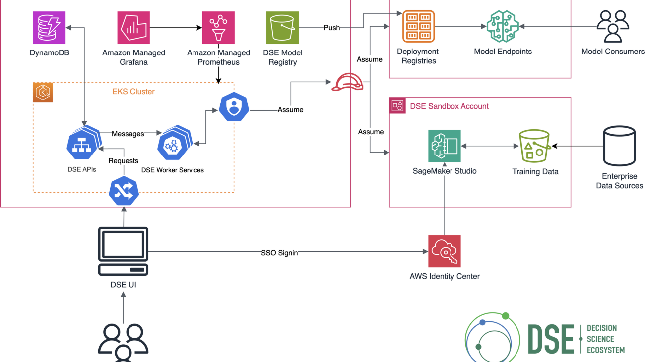


 Senaka Ariyasinghe is a Senior Partner Solutions Architect at AWS. He collaborates with Global Systems Integrators to drive cloud innovation across the Asia-Pacific and Japan region. He specializes in helping AWS partners develop and implement scalable, well-architected solutions, with particular emphasis on generative AI, machine learning, cloud migration strategies, and the modernization of enterprise applications.
 Senthil Nathan is a Senior Partner Solutions Architect working with Global Systems Integrators at AWS. In his role, Senthil works closely with global partners to help them maximize the value and potential of the AWS Cloud landscape. He is passionate about using the transformative power of cloud computing and emerging technologies to drive innovation and business impact.
 Deependra Shekhawat is a Senior Energy and Utilities Industry Specialist Solutions Architect based in Sydney, Australia. In his role, Deependra helps energy companies across the Asia-Pacific and Japan region use cloud technologies to drive sustainability and operational efficiency. He specializes in creating robust data foundations and advanced workflows that enable organizations to harness the power of big data, analytics, and machine learning for solving critical industry challenges.
 Aaron Sempf is Next Gen Tech Lead for the AWS Partner Organization in Asia-Pacific and Japan. With over 20 years in distributed system engineering design and development, he focuses on solving for large-scale complex integration and event-driven systems. In his spare time, he can be found coding prototypes for autonomous robots, IoT devices, distributed solutions, and designing agentic architecture patterns for generative AI-assisted business automation.
 Ozan Eken is a Product Manager at AWS, passionate about building cutting-edge generative AI and graph analytics products. With a focus on simplifying complex data challenges, Ozan helps customers unlock deeper insights and accelerate innovation. Outside of work, he enjoys trying new foods, exploring different countries, and watching soccer.
 JaiPrakash Dave is a Partner Solutions Architect working with Global Systems Integrators at AWS based in India. In his role, JaiPrakash guides AWS partners in the India region to design and scale well-architected solutions, focusing on generative AI, machine learning, DevOps, and application and data modernization initiatives.