The Atari57 suite of games is a long-standing benchmark to gauge agent performance across a wide range of tasks. Weve developed Agent57, the first deep reinforcement learning agent to obtain a score that is above the human baseline on all 57 Atari 2600 games. Agent57 combines an algorithm for efficient exploration with a meta-controller that adapts the exploration and long vs. short-term behaviour of the agent.Read More
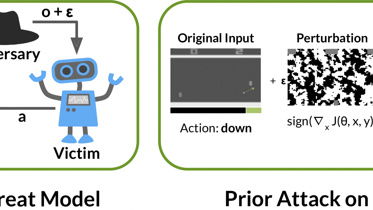
Physically Realistic Attacks on Deep Reinforcement Learning
Deep reinforcement learning (RL) has achieved superhuman performance in
problems ranging from data center cooling to video games. RL policies
may soon be widely deployed, with research underway in autonomous driving,
negotiation and automated trading. Many potential applications are
safety-critical: automated trading failures caused Knight Capital to lose
USD 460M, while faulty autonomous vehicles have resulted in loss of
life.
Consequently, it is critical that RL policies are robust: both to naturally
occurring distribution shift, and to malicious attacks by adversaries.
Unfortunately, we find that RL policies which perform at a high-level in normal
situations can harbor serious vulnerabilities which can be exploited by an
adversary.
Introduction to Quantization on PyTorch
It’s important to make efficient use of both server-side and on-device compute resources when developing machine learning applications. To support more efficient deployment on servers and edge devices, PyTorch added a support for model quantization using the familiar eager mode Python API.
Quantization leverages 8bit integer (int8) instructions to reduce the model size and run the inference faster (reduced latency) and can be the difference between a model achieving quality of service goals or even fitting into the resources available on a mobile device. Even when resources aren’t quite so constrained it may enable you to deploy a larger and more accurate model. Quantization is available in PyTorch starting in version 1.3 and with the release of PyTorch 1.4 we published quantized models for ResNet, ResNext, MobileNetV2, GoogleNet, InceptionV3 and ShuffleNetV2 in the PyTorch torchvision 0.5 library.
This blog post provides an overview of the quantization support on PyTorch and its incorporation with the TorchVision domain library.
What is Quantization?
Quantization refers to techniques for doing both computations and memory accesses with lower precision data, usually int8 compared to floating point implementations. This enables performance gains in several important areas:
- 4x reduction in model size;
- 2-4x reduction in memory bandwidth;
- 2-4x faster inference due to savings in memory bandwidth and faster compute with int8 arithmetic (the exact speed up varies depending on the hardware, the runtime, and the model).
Quantization does not however come without additional cost. Fundamentally quantization means introducing approximations and the resulting networks have slightly less accuracy. These techniques attempt to minimize the gap between the full floating point accuracy and the quantized accuracy.
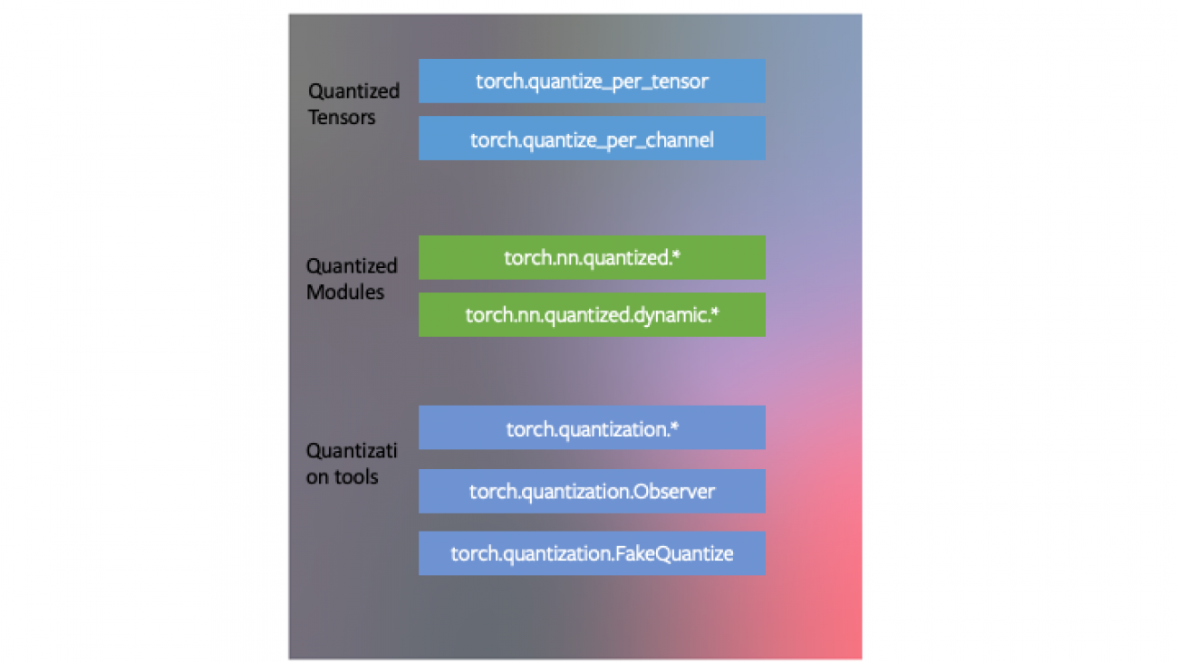
We designed quantization to fit into the PyTorch framework. The means that:
- PyTorch has data types corresponding to quantized tensors, which share many of the features of tensors.
- One can write kernels with quantized tensors, much like kernels for floating point tensors to customize their implementation. PyTorch supports quantized modules for common operations as part of the
torch.nn.quantizedandtorch.nn.quantized.dynamicname-space. - Quantization is compatible with the rest of PyTorch: quantized models are traceable and scriptable. The quantization method is virtually identical for both server and mobile backends. One can easily mix quantized and floating point operations in a model.
- Mapping of floating point tensors to quantized tensors is customizable with user defined observer/fake-quantization blocks. PyTorch provides default implementations that should work for most use cases.

We developed three techniques for quantizing neural networks in PyTorch as part of quantization tooling in the torch.quantization name-space.
The Three Modes of Quantization Supported in PyTorch starting version 1.3
-
Dynamic Quantization
The easiest method of quantization PyTorch supports is called dynamic quantization. This involves not just converting the weights to int8 – as happens in all quantization variants – but also converting the activations to int8 on the fly, just before doing the computation (hence “dynamic”). The computations will thus be performed using efficient int8 matrix multiplication and convolution implementations, resulting in faster compute. However, the activations are read and written to memory in floating point format.
- PyTorch API: we have a simple API for dynamic quantization in PyTorch.
torch.quantization.quantize_dynamictakes in a model, as well as a couple other arguments, and produces a quantized model! Our end-to-end tutorial illustrates this for a BERT model; while the tutorial is long and contains sections on loading pre-trained models and other concepts unrelated to quantization, the part the quantizes the BERT model is simply:
import torch.quantization quantized_model = torch.quantization.quantize_dynamic(model, {torch.nn.Linear}, dtype=torch.qint8) - PyTorch API: we have a simple API for dynamic quantization in PyTorch.
-
Post-Training Static Quantization
One can further improve the performance (latency) by converting networks to use both integer arithmetic and int8 memory accesses. Static quantization performs the additional step of first feeding batches of data through the network and computing the resulting distributions of the different activations (specifically, this is done by inserting “observer” modules at different points that record these distributions). This information is used to determine how specifically the different activations should be quantized at inference time (a simple technique would be to simply divide the entire range of activations into 256 levels, but we support more sophisticated methods as well). Importantly, this additional step allows us to pass quantized values between operations instead of converting these values to floats – and then back to ints – between every operation, resulting in a significant speed-up.
With this release, we’re supporting several features that allow users to optimize their static quantization:
- Observers: you can customize observer modules which specify how statistics are collected prior to quantization to try out more advanced methods to quantize your data.
- Operator fusion: you can fuse multiple operations into a single operation, saving on memory access while also improving the operation’s numerical accuracy.
- Per-channel quantization: we can independently quantize weights for each output channel in a convolution/linear layer, which can lead to higher accuracy with almost the same speed.
-
PyTorch API:
- To fuse modules, we have
torch.quantization.fuse_modules - Observers are inserted using
torch.quantization.prepare - Finally, quantization itself is done using
torch.quantization.convert
- To fuse modules, we have
We have a tutorial with an end-to-end example of quantization (this same tutorial also covers our third quantization method, quantization-aware training), but because of our simple API, the three lines that perform post-training static quantization on the pre-trained model
myModelare:# set quantization config for server (x86) deploymentmyModel.qconfig = torch.quantization.get_default_config('fbgemm') # insert observers torch.quantization.prepare(myModel, inplace=True) # Calibrate the model and collect statistics # convert to quantized version torch.quantization.convert(myModel, inplace=True) -
Quantization Aware Training
Quantization-aware training(QAT) is the third method, and the one that typically results in highest accuracy of these three. With QAT, all weights and activations are “fake quantized” during both the forward and backward passes of training: that is, float values are rounded to mimic int8 values, but all computations are still done with floating point numbers. Thus, all the weight adjustments during training are made while “aware” of the fact that the model will ultimately be quantized; after quantizing, therefore, this method usually yields higher accuracy than the other two methods.
-
PyTorch API:
torch.quantization.prepare_qatinserts fake quantization modules to model quantization.- Mimicking the static quantization API,
torch.quantization.convertactually quantizes the model once training is complete.
For example, in the end-to-end example, we load in a pre-trained model as
qat_model, then we simply perform quantization-aware training using:# specify quantization config for QAT qat_model.qconfig=torch.quantization.get_default_qat_qconfig('fbgemm') # prepare QAT torch.quantization.prepare_qat(qat_model, inplace=True) # convert to quantized version, removing dropout, to check for accuracy on each epochquantized_model=torch.quantization.convert(qat_model.eval(), inplace=False) -
Device and Operator Support
Quantization support is restricted to a subset of available operators, depending on the method being used, for a list of supported operators, please see the documentation at https://pytorch.org/docs/stable/quantization.html.
The set of available operators and the quantization numerics also depend on the backend being used to run quantized models. Currently quantized operators are supported only for CPU inference in the following backends: x86 and ARM. Both the quantization configuration (how tensors should be quantized and the quantized kernels (arithmetic with quantized tensors) are backend dependent. One can specify the backend by doing:
import torchbackend='fbgemm'
# 'fbgemm' for server, 'qnnpack' for mobile
my_model.qconfig = torch.quantization.get_default_qconfig(backend)
# prepare and convert model
# Set the backend on which the quantized kernels need to be run
torch.backends.quantized.engine=backend
However, quantization aware training occurs in full floating point and can run on either GPU or CPU. Quantization aware training is typically only used in CNN models when post training static or dynamic quantization doesn’t yield sufficient accuracy. This can occur with models that are highly optimized to achieve small size (such as Mobilenet).
Integration in torchvision
We’ve also enabled quantization for some of the most popular models in torchvision: Googlenet, Inception, Resnet, ResNeXt, Mobilenet and Shufflenet. We have upstreamed these changes to torchvision in three forms:
- Pre-trained quantized weights so that you can use them right away.
- Quantization ready model definitions so that you can do post-training quantization or quantization aware training.
- A script for doing quantization aware training — which is available for any of these model though, as you will learn below, we only found it necessary for achieving accuracy with Mobilenet.
- We also have a tutorial showing how you can do transfer learning with quantization using one of the torchvision models.
Choosing an approach
The choice of which scheme to use depends on multiple factors:
- Model/Target requirements: Some models might be sensitive to quantization, requiring quantization aware training.
- Operator/Backend support: Some backends require fully quantized operators.
Currently, operator coverage is limited and may restrict the choices listed in the table below:
The table below provides a guideline.
| Model Type | Preferred scheme | Why |
|---|---|---|
| LSTM/RNN | Dynamic Quantization | Throughput dominated by compute/memory bandwidth for weights |
| BERT/Transformer | Dynamic Quantization | Throughput dominated by compute/memory bandwidth for weights |
| CNN | Static Quantization | Throughput limited by memory bandwidth for activations |
| CNN | Quantization Aware Training | In the case where accuracy can’t be achieved with static quantization |
Performance Results
Quantization provides a 4x reduction in the model size and a speedup of 2x to 3x compared to floating point implementations depending on the hardware platform and the model being benchmarked. Some sample results are:
| Model | Float Latency (ms) | Quantized Latency (ms) | Inference Performance Gain | Device | Notes |
| BERT | 581 | 313 | 1.8x | Xeon-D2191 (1.6GHz) | Batch size = 1, Maximum sequence length= 128, Single thread, x86-64, Dynamic quantization |
| Resnet-50 | 214 | 103 | 2x | Xeon-D2191 (1.6GHz) | Single thread, x86-64, Static quantization |
| Mobilenet-v2 | 97 | 17 | 5.7x | Samsung S9 | Static quantization, Floating point numbers are based on Caffe2 run-time and are not optimized |
Accuracy results
We also compared the accuracy of static quantized models with the floating point models on Imagenet. For dynamic quantization, we compared the F1 score of BERT on the GLUE benchmark for MRPC.
Computer Vision Model accuracy
| Model | Top-1 Accuracy (Float) | Top-1 Accuracy (Quantized) | Quantization scheme |
| Googlenet | 69.8 | 69.7 | Static post training quantization |
| Inception-v3 | 77.5 | 77.1 | Static post training quantization |
| ResNet-18 | 69.8 | 69.4 | Static post training quantization |
| Resnet-50 | 76.1 | 75.9 | Static post training quantization |
| ResNext-101 32x8d | 79.3 | 79 | Static post training quantization |
| Mobilenet-v2 | 71.9 | 71.6 | Quantization Aware Training |
| Shufflenet-v2 | 69.4 | 68.4 | Static post training quantization |
Speech and NLP Model accuracy
| Model | F1 (GLUEMRPC) Float | F1 (GLUEMRPC) Quantized | Quantization scheme |
| BERT | 0.902 | 0.895 | Dynamic quantization |
Conclusion
To get started on quantizing your models in PyTorch, start with the tutorials on the PyTorch website. If you are working with sequence data start with dynamic quantization for LSTM, or BERT. If you are working with image data then we recommend starting with the transfer learning with quantization tutorial. Then you can explore static post training quantization. If you find that the accuracy drop with post training quantization is too high, then try quantization aware training.
If you run into issues you can get community help by posting in at discuss.pytorch.org, use the quantization category for quantization related issues.
This post is authored by Raghuraman Krishnamoorthi, James Reed, Min Ni, Chris Gottbrath and Seth Weidman. Special thanks to Jianyu Huang, Lingyi Liu and Haixin Liu for producing quantization metrics included in this post.
Further reading:
- PyTorch quantization presentation at Neurips: (https://research.fb.com/wp-content/uploads/2019/12/2.-Quantization.pptx)
- Quantized Tensors (https://github.com/pytorch/pytorch/wiki/
Introducing-Quantized-Tensor) - Quantization RFC on Github (https://github.com/pytorch/pytorch/
issues/18318)
Neural networks facilitate optimization in the search for new materials
When searching through theoretical lists of possible new materials for particular applications, such as batteries or other energy-related devices, there are often millions of potential materials that could be considered, and multiple criteria that need to be met and optimized at once. Now, researchers at MIT have found a way to dramatically streamline the discovery process, using a machine learning system.
As a demonstration, the team arrived at a set of the eight most promising materials, out of nearly 3 million candidates, for an energy storage system called a flow battery. This culling process would have taken 50 years by conventional analytical methods, they say, but they accomplished it in five weeks.
The findings are reported in the journal ACS Central Science, in a paper by MIT professor of chemical engineering Heather Kulik, Jon Paul Janet PhD ’19, Sahasrajit Ramesh, and graduate student Chenru Duan.
The study looked at a set of materials called transition metal complexes. These can exist in a vast number of different forms, and Kulik says they “are really fascinating, functional materials that are unlike a lot of other material phases. The only way to understand why they work the way they do is to study them using quantum mechanics.”
To predict the properties of any one of millions of these materials would require either time-consuming and resource-intensive spectroscopy and other lab work, or time-consuming, highly complex physics-based computer modeling for each possible candidate material or combination of materials. Each such study could consume hours to days of work.
Instead, Kulik and her team took a small number of different possible materials and used them to teach an advanced machine-learning neural network about the relationship between the materials’ chemical compositions and their physical properties. That knowledge was then applied to generate suggestions for the next generation of possible materials to be used for the next round of training of the neural network. Through four successive iterations of this process, the neural network improved significantly each time, until reaching a point where it was clear that further iterations would not yield any further improvements.
This iterative optimization system greatly streamlined the process of arriving at potential solutions that satisfied the two conflicting criteria being sought. This kind of process of finding the best solutions in situations, where improving one factor tends to worsen the other, is known as a Pareto front, representing a graph of the points such that any further improvement of one factor would make the other worse. In other words, the graph represents the best possible compromise points, depending on the relative importance assigned to each factor.
Training typical neural networks requires very large data sets, ranging from thousands to millions of examples, but Kulik and her team were able to use this iterative process, based on the Pareto front model, to streamline the process and provide reliable results using only the few hundred samples.
In the case of screening for the flow battery materials, the desired characteristics were in conflict, as is often the case: The optimum material would have high solubility and a high energy density (the ability to store energy for a given weight). But increasing solubility tends to decrease the energy density, and vice versa.
Not only was the neural network able to rapidly come up with promising candidates, it also was able to assign levels of confidence to its different predictions through each iteration, which helped to allow the refinement of the sample selection at each step. “We developed a better than best-in-class uncertainty quantification technique for really knowing when these models were going to fail,” Kulik says.
The challenge they chose for the proof-of-concept trial was materials for use in redox flow batteries, a type of battery that holds promise for large, grid-scale batteries that could play a significant role in enabling clean, renewable energy. Transition metal complexes are the preferred category of materials for such batteries, Kulik says, but there are too many possibilities to evaluate by conventional means. They started out with a list of 3 million such complexes before ultimately whittling that down to the eight good candidates, along with a set of design rules that should enable experimentalists to explore the potential of these candidates and their variations.
“Through that process, the neural net both gets increasingly smarter about the [design] space, but also increasingly pessimistic that anything beyond what we’ve already characterized can further improve on what we already know,” she says.
Apart from the specific transition metal complexes suggested for further investigation using this system, she says, the method itself could have much broader applications. “We do view it as the framework that can be applied to any materials design challenge where you’re really trying to address multiple objectives at once. You know, all of the most interesting materials design challenges are ones where you have one thing you’re trying to improve, but improving that worsens another. And for us, the redox flow battery redox couple was just a good demonstration of where we think we can go with this machine learning and accelerated materials discovery.”
For example, optimizing catalysts for various chemical and industrial processes is another kind of such complex materials search, Kulik says. Presently used catalysts often involve rare and expensive elements, so finding similarly effective compounds based on abundant and inexpensive materials could be a significant advantage.
“This paper represents, I believe, the first application of multidimensional directed improvement in the chemical sciences,” she says. But the long-term significance of the work is in the methodology itself, because of things that might not be possible at all otherwise. “You start to realize that even with parallel computations, these are cases where we wouldn’t have come up with a design principle in any other way. And these leads that are coming out of our work, these are not necessarily at all ideas that were already known from the literature or that an expert would have been able to point you to.”
“This is a beautiful combination of concepts in statistics, applied math, and physical science that is going to be extremely useful in engineering applications,” says George Schatz, a professor of chemistry and of chemical and biological engineering at Northwestern University, who was not associated with this work. He says this research addresses “how to do machine learning when there are multiple objectives. Kulik’s approach uses leading edge methods to train an artificial neural network that is used to predict which combination of transition metal ions and organic ligands will be best for redox flow battery electrolytes.”
Schatz says “this method can be used in many different contexts, so it has the potential to transform machine learning, which is a major activity around the world.”
The work was supported by the Office of Naval Research, the Defense Advanced Research Projects Agency (DARPA), the U.S. Department of Energy, the Burroughs Wellcome Fund, and the AAAS Mar ion Milligan Mason Award.
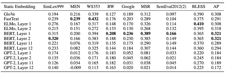
BERT, ELMo, & GPT-2: How Contextual are Contextualized Word Representations?
Incorporating context into word embeddings – as exemplified by BERT, ELMo, and GPT-2 – has proven to be a watershed idea in NLP. Replacing static vectors (e.g., word2vec) with contextualized word representations has led to significant improvements on virtually every NLP task.
But just how contextual are these contextualized representations?
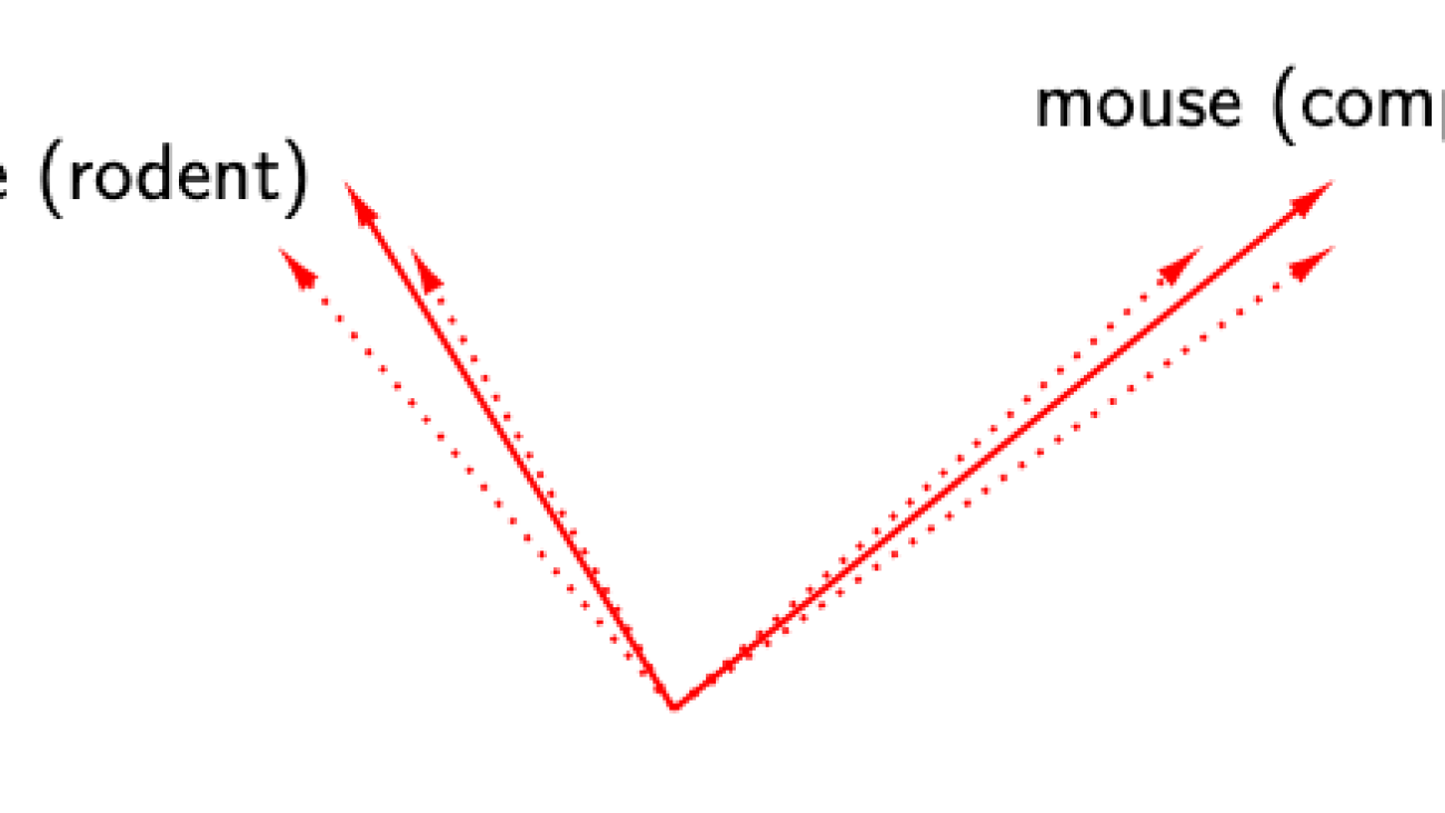
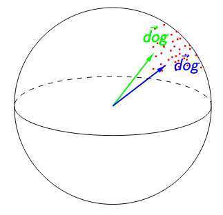
Consider the word ‘mouse’. It has multiple word senses, one referring to a rodent and another to a device. Does BERT effectively create one representation of ‘mouse’ per word sense (left) ? Or does BERT create infinitely many representations of ‘mouse’, each highly specific to its context (right)?
![]()
![]()
In our EMNLP 2019 paper, “How Contextual are Contextualized Word Representations?”, we tackle these questions and arrive at some surprising conclusions:
-
In all layers of BERT, ELMo, and GPT-2, the representations of all words are anisotropic: they occupy a narrow cone in the embedding space instead of being distributed throughout.
-
In all three models, upper layers produce more context-specific representations than lower layers; however, the models contextualize words very differently from one another.
-
If a word’s contextualized representations were not at all contextual, we’d expect 100% of their variance to be explained by a static embedding. Instead, we find that – on average – less than 5% of the variance can be explained by a static embedding.1
-
We can create a new type of static embedding for each word by taking the first principal component of its contextualized representations in a lower layer of BERT. Static embeddings created this way outperform GloVe and FastText on benchmarks like solving word analogies!2
Going back to our example, this means that BERT creates highly context-specific representations of the word ‘mouse’ instead of creating one per word sense. Any static embedding of ‘mouse’ would account for very little of the variance in its contextualized representations. However, if we picked the vector that did maximize the variance explained, we would get a static embedding that is much better than the one provided by GloVe or FastText!3
Measures of Contextuality
What does contextuality look like? Consider these two sentences:
A panda dog runs.
A dog is trying to get bacon off its back.
== implies that there is no contextualization (i.e., what we’d get with word2vec).
!= implies that there is some contextualization. The difficulty lies in quantifying the extent to which this occurs. Since there is no definitive measure of contextuality, we propose three new ones:
-
Self-Similarity (SelfSim): The average cosine similarity of a word with itself across all the contexts in which it appears, where representations of the word are drawn from the same layer of a given model. For example, we would take the mean of cos(, ) over all unique pairs to calculate (‘dog’).
-
Intra-Sentence Similarity (IntraSim): The average cosine similarity between a word and its context. For the first sentence, where context vector :
helps us discern whether the contextualization is naive – simply making each word more similar to its neighbors – or whether it is more nuanced, recognizing that words occurring in the same context can affect each other while still having distinct semantics.
-
Maximum Explainable Variance (MEV): The proportion of variance in a word’s representations that can be explained by their first principal component. For example, (‘dog’) would be the proportion of variance explained by the first principal component of , , and every other instance of ‘dog’ in the data. (‘dog’) = 1 would imply that there was no contextualization: a static embedding could replace all the contextualized representations. Conversely, if (‘dog’) were close to 0, then a static embedding could explain almost none of the variance.
Note that each of these measures is calculated for a given layer of a given model, since each layer has its own representation space. For example, the word ‘dog’ has different self-similarity values in Layer 1 of BERT and Layer 2 of BERT.
Adjusting for Anisotropy
When discussing contextuality, it is important to consider the isotropy of embeddings (i.e., whether they’re uniformly distributed in all directions).
In both figures below, (‘dog’) = 0.95. The image on the left suggests that ‘dog’ is poorly contextualized. Not only are its representations nearly identical across all the contexts in which it appears, but the high isotropy of the representation space suggests that a self-similarity of 0.95 is exceptionally high. The image on the right suggests the opposite: because any two words have a cosine similarity over 0.95, ‘dog’ having a self-similarity of 0.95 is no longer impressive. Relative to other words, ‘dog’ would be considered highly contextualized!
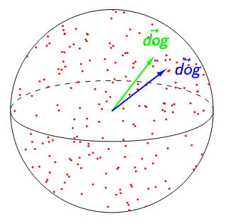 vs.
vs.
To adjust for anisotropy, we calculate anisotropic baselines for each of our measures and subtract each baseline from the respective raw measure.4
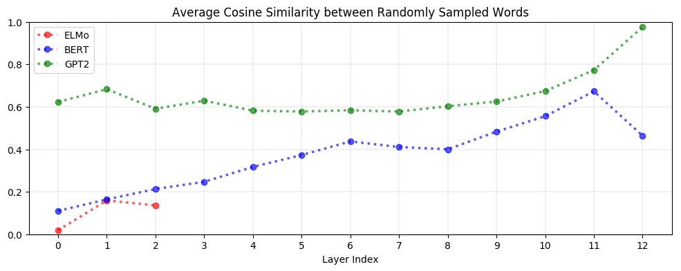
But is it even necessary to adjust for anisotropy? Yes! As seen below, upper layers of BERT and GPT-2 are extremely anisotropic, suggesting that high anisotropy is inherent to – or at least a consequence of – the process of contextualization:
Context-Specificity
On average, contextualized representations are more context-specific in higher layers. As seen below, the decrease in self-similarity is almost monotonic. This is analogous to how upper layers of LSTMs trained on NLP tasks learn more task-specific representations (Liu et al., 2019). GPT-2 is the most context-specific; representations in its last layer are almost maximally context-specific.
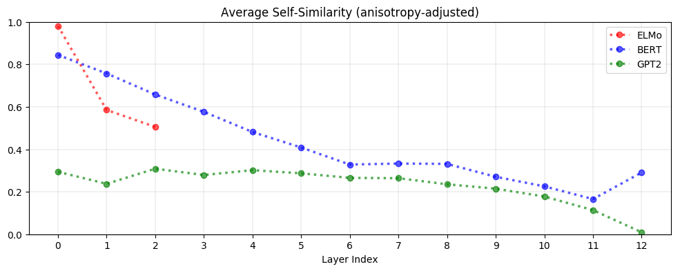
Stopwords such as ‘the’ have among the lowest self-similarity (i.e., the most context-specific representations). The variety of contexts a word appears in, rather than its inherent polysemy, is what drives variation in its contextualized representations. This suggests that ELMo, BERT, and GPT-2 are not simply assigning one representation per word sense; otherwise, there would not be so much variation in the representations of words with so few word senses.
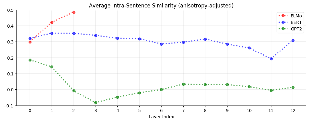
Context-specificity manifests very differently in ELMo, BERT, and GPT-2. As seen below, in ELMo, words in the same sentence are more similar to one another in upper layers. In BERT, words in the same sentence are more dissimilar to one another in upper layers but are on average more similar to each other than two random words. In contrast, for GPT-2, word representations in the same sentence are no more similar to each other than randomly sampled words. This suggests that BERT and GPT-2’s contextualization are more nuanced than ELMo’s, as they seem to recognize that words appearing in the same context do not necessarily have a similar meaning.
Static vs. Contextualized
On average, less than 5% of the variance in a word’s contextualized representations can be explained by a static embedding. If a word’s contextualized representations were not at all contextual, we would expect their first principal component to explain 100% of the variance. Instead, less than 5% of the variance can be explained on average. This 5% threshold represents the best-case scenario, where the static embedding is the first principal component. There is no theoretical guarantee that a GloVe vector, for example, is similar to the static embedding that maximizes the variance explained. This suggests that BERT, ELMo, and GPT-2 are not simply assigning one embedding per word sense: otherwise, the proportion of variance explained would be much higher.
Principal components of contextualized representations in lower layers of BERT outperform GloVe and FastText on many static embedding benchmarks. This method takes the previous finding to its logical conclusion: what if we created a new type of static embedding for each word by simply taking the first principal component of its contextualized representations? It turns out that this works surprisingly well. If we use representations from lower layers of BERT, these principal component embeddings outperform GloVe and FastText on benchmark tasks covering semantic similarity, analogy solving, and concept categorization (see table below).
For all three models, principal component embeddings created from lower layers are more effective than those created from upper layers. Those created using GPT-2 perform markedly worse than those from ELMo and BERT. Given that upper layers are much more context-specific than lower layers, and given that GPT-2’s representations are more context-specific, this suggests that principal components of less context-specific representations are more effective on these tasks.
Conclusion
In ELMo, BERT, and GPT-2, upper layers produce more context-specific representations than lower layers. However, these models contextualize words very differently from one another: after adjusting for anisotropy, the similarity between words in the same sentence is highest in ELMo but almost non-existent in GPT-2.
On average, less than 5% of the variance in a word’s contextualized representations can be explained by a static embedding. Even in the best-case scenario, static word embeddings would thus be a poor replacement for contextualized ones. Still, contextualized representations can be used to create a more powerful type of static embedding: principal components of contextualized representations in lower layers of BERT are much better than GloVe and FastText! If you’re interested in reading more along these lines, check out:
- The Dark Secrets of BERT (Rogers et al., 2019)
- Evolution of Representations in the Transformer (Voita et al., 2019)
- Cross-Lingual Alignment of Contextual Word Embeddings (Schuster et al., 2019)
- The Illustrated BERT, ELMo, and co. (Alammar, 2019)
Acknowledgements
Many thanks to Anna Rogers for live-tweeting this paper during EMNLP 2019. Special thanks to John Hewitt, Nelson Liu, and Krishnapriya Vishnubhotla for their comments on this blog post.
-
This was calculated after adjusting for the effect of anisotropy. ↩
-
The fact that arithmetic operators can be applied to embedding spaces is a hallmark of word vectors. Still, the ability to solve word analogies should not be treated as a perfect proxy for embedding quality (see Schluter, 2018; Rogers et al., 2017). To understand the theory behind when word analogies hold, see Ethayarajh et al., 2019. ↩
-
Provided we use the contextualized representations from lower layers of BERT (see the section titled ‘Static vs. Contextualized’). ↩
-
For self-similarity and intra-sentence similarity, the baseline is the average cosine similarity between randomly sampled word representations (of different words) from a given layer’s representation space. For , the baseline is the variance explained by the first principal component of uniformly randomly sampled representations. See the paper for details. ↩
System trains driverless cars in simulation before they hit the road
A simulation system invented at MIT to train driverless cars creates a photorealistic world with infinite steering possibilities, helping the cars learn to navigate a host of worse-case scenarios before cruising down real streets.
Control systems, or “controllers,” for autonomous vehicles largely rely on real-world datasets of driving trajectories from human drivers. From these data, they learn how to emulate safe steering controls in a variety of situations. But real-world data from hazardous “edge cases,” such as nearly crashing or being forced off the road or into other lanes, are — fortunately — rare.
Some computer programs, called “simulation engines,” aim to imitate these situations by rendering detailed virtual roads to help train the controllers to recover. But the learned control from simulation has never been shown to transfer to reality on a full-scale vehicle.
The MIT researchers tackle the problem with their photorealistic simulator, called Virtual Image Synthesis and Transformation for Autonomy (VISTA). It uses only a small dataset, captured by humans driving on a road, to synthesize a practically infinite number of new viewpoints from trajectories that the vehicle could take in the real world. The controller is rewarded for the distance it travels without crashing, so it must learn by itself how to reach a destination safely. In doing so, the vehicle learns to safely navigate any situation it encounters, including regaining control after swerving between lanes or recovering from near-crashes.
In tests, a controller trained within the VISTA simulator safely was able to be safely deployed onto a full-scale driverless car and to navigate through previously unseen streets. In positioning the car at off-road orientations that mimicked various near-crash situations, the controller was also able to successfully recover the car back into a safe driving trajectory within a few seconds. A paper describing the system has been published in IEEE Robotics and Automation Letters and will be presented at the upcoming ICRA conference in May.
“It’s tough to collect data in these edge cases that humans don’t experience on the road,” says first author Alexander Amini, a PhD student in the Computer Science and Artificial Intelligence Laboratory (CSAIL). “In our simulation, however, control systems can experience those situations, learn for themselves to recover from them, and remain robust when deployed onto vehicles in the real world.”
The work was done in collaboration with the Toyota Research Institute. Joining Amini on the paper are Igor Gilitschenski, a postdoc in CSAIL; Jacob Phillips, Julia Moseyko, and Rohan Banerjee, all undergraduates in CSAIL and the Department of Electrical Engineering and Computer Science; Sertac Karaman, an associate professor of aeronautics and astronautics; and Daniela Rus, director of CSAIL and the Andrew and Erna Viterbi Professor of Electrical Engineering and Computer Science.
Data-driven simulation
Historically, building simulation engines for training and testing autonomous vehicles has been largely a manual task. Companies and universities often employ teams of artists and engineers to sketch virtual environments, with accurate road markings, lanes, and even detailed leaves on trees. Some engines may also incorporate the physics of a car’s interaction with its environment, based on complex mathematical models.
But since there are so many different things to consider in complex real-world environments, it’s practically impossible to incorporate everything into the simulator. For that reason, there’s usually a mismatch between what controllers learn in simulation and how they operate in the real world.
Instead, the MIT researchers created what they call a “data-driven” simulation engine that synthesizes, from real data, new trajectories consistent with road appearance, as well as the distance and motion of all objects in the scene.
They first collect video data from a human driving down a few roads and feed that into the engine. For each frame, the engine projects every pixel into a type of 3D point cloud. Then, they place a virtual vehicle inside that world. When the vehicle makes a steering command, the engine synthesizes a new trajectory through the point cloud, based on the steering curve and the vehicle’s orientation and velocity.
Then, the engine uses that new trajectory to render a photorealistic scene. To do so, it uses a convolutional neural network — commonly used for image-processing tasks — to estimate a depth map, which contains information relating to the distance of objects from the controller’s viewpoint. It then combines the depth map with a technique that estimates the camera’s orientation within a 3D scene. That all helps pinpoint the vehicle’s location and relative distance from everything within the virtual simulator.
Based on that information, it reorients the original pixels to recreate a 3D representation of the world from the vehicle’s new viewpoint. It also tracks the motion of the pixels to capture the movement of the cars and people, and other moving objects, in the scene. “This is equivalent to providing the vehicle with an infinite number of possible trajectories,” Rus says. “Because when we collect physical data, we get data from the specific trajectory the car will follow. But we can modify that trajectory to cover all possible ways of and environments of driving. That’s really powerful.”
Reinforcement learning from scratch
Traditionally, researchers have been training autonomous vehicles by either following human defined rules of driving or by trying to imitate human drivers. But the researchers make their controller learn entirely from scratch under an “end-to-end” framework, meaning it takes as input only raw sensor data — such as visual observations of the road — and, from that data, predicts steering commands at outputs.
“We basically say, ‘Here’s an environment. You can do whatever you want. Just don’t crash into vehicles, and stay inside the lanes,’” Amini says.
This requires “reinforcement learning” (RL), a trial-and-error machine-learning technique that provides feedback signals whenever the car makes an error. In the researchers’ simulation engine, the controller begins by knowing nothing about how to drive, what a lane marker is, or even other vehicles look like, so it starts executing random steering angles. It gets a feedback signal only when it crashes. At that point, it gets teleported to a new simulated location and has to execute a better set of steering angles to avoid crashing again. Over 10 to 15 hours of training, it uses these sparse feedback signals to learn to travel greater and greater distances without crashing.
After successfully driving 10,000 kilometers in simulation, the authors apply that learned controller onto their full-scale autonomous vehicle in the real world. The researchers say this is the first time a controller trained using end-to-end reinforcement learning in simulation has successful been deployed onto a full-scale autonomous car. “That was surprising to us. Not only has the controller never been on a real car before, but it’s also never even seen the roads before and has no prior knowledge on how humans drive,” Amini says.
Forcing the controller to run through all types of driving scenarios enabled it to regain control from disorienting positions — such as being half off the road or into another lane — and steer back into the correct lane within several seconds. “And other state-of-the-art controllers all tragically failed at that, because they never saw any data like this in training,” Amini says.
Next, the researchers hope to simulate all types of road conditions from a single driving trajectory, such as night and day, and sunny and rainy weather. They also hope to simulate more complex interactions with other vehicles on the road. “What if other cars start moving and jump in front of the vehicle?” Rus says. “Those are complex, real-world interactions we want to start testing.”
Combining knowledge graphs, quickly and accurately
Novel cross-graph-attention and self-attention mechanisms enable state-of-the-art performance.Read More
How Amazon Fellow Inderjit Dhillon is improving shopping discovery on Amazon
Developing machine learning frameworks that can enhance context-aware AI has been an area of focus for Dhillon’s entire career.Read More
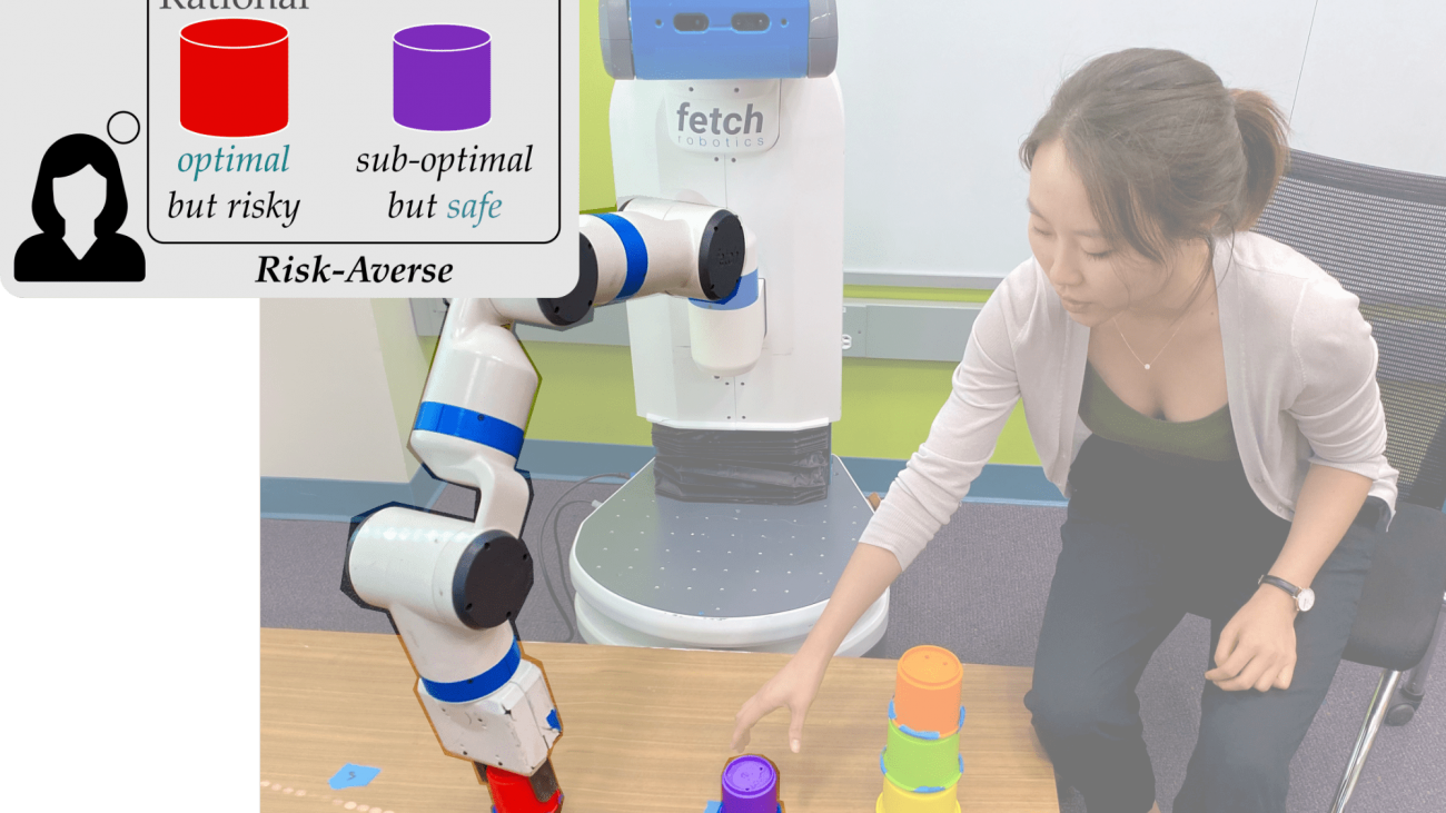
When Humans Aren’t Optimal: Robots that Collaborate with Risk-Aware Humans
A key component of human-robot collaboration is the ability for robots to predict human behavior. Robots do this by building models of human decision making. One way to model humans is to pretend that they are also robots, and assume users will always choose the optimal action that leads to the best outcomes. It’s also possible to account for human limitations, and relax this assumption so that the human is noisily rational (their actions will usually lead to the ideal outcome, but are also somewhat random).
Both of these models work well when humans receive deterministic rewards: e.g., gaining either or with certainty. But in real-world scenarios, humans often need to make decisions under risk and uncertainty: i.e., gaining all the time or about % of the time. In these uncertain settings, humans tend to make suboptimal choices and select the risk-averse option — even though it leads to worse expected outcomes! Our insight is that we should take risk into account when modeling humans in order to better understand and predict their behavior.
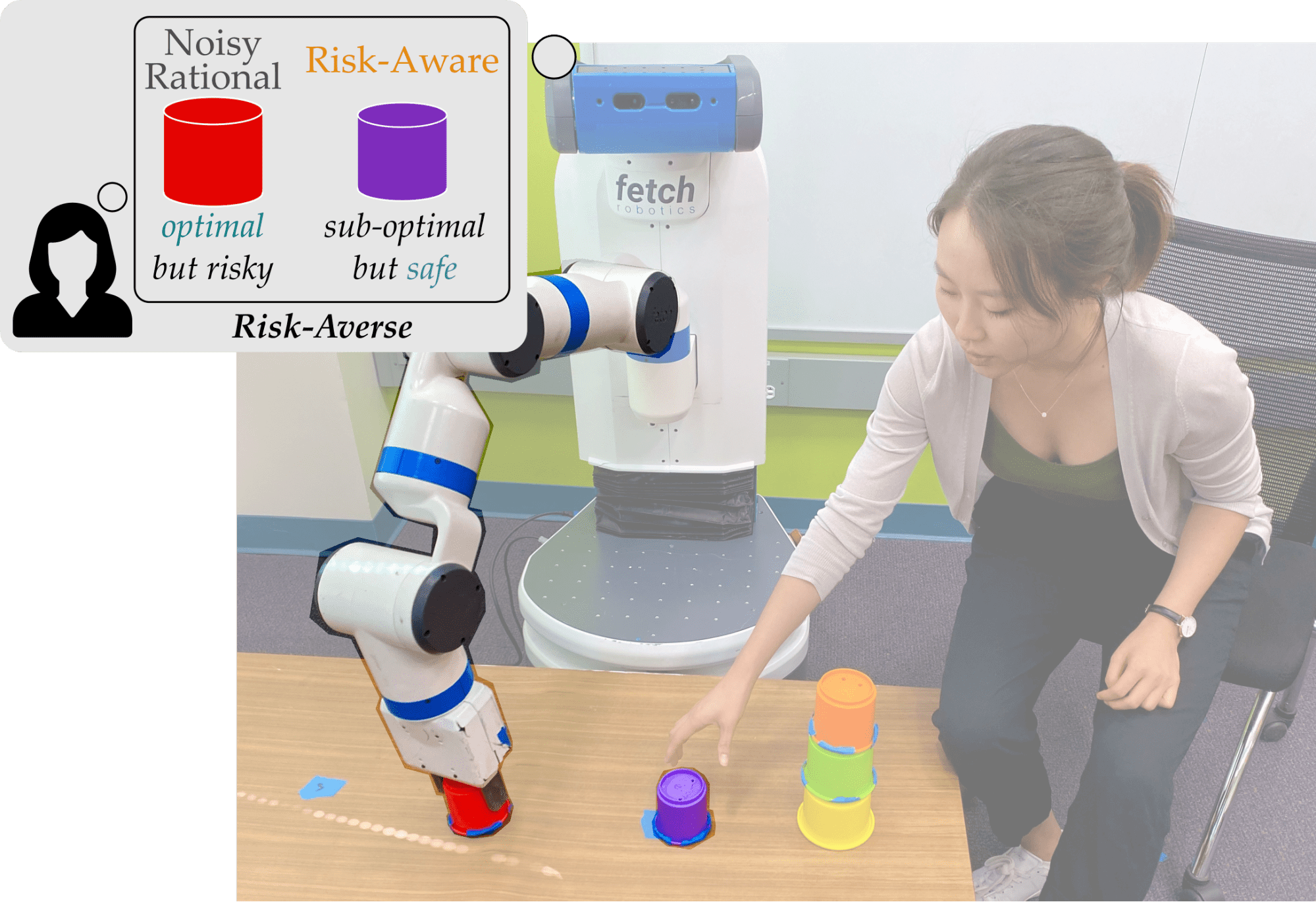
In this blog post, we describe our Risk-Aware model and compare it to the state-of-the-art Noisy Rational model. We also summarize the results from user studies that test how well Risk-Aware robots predict human behavior, and how Risk-Aware robots can leverage this model to improve safety and efficiency in human-robot collaboration. Please refer to our paper and the accompanying video for more details and footage of the experiments.
Motivation
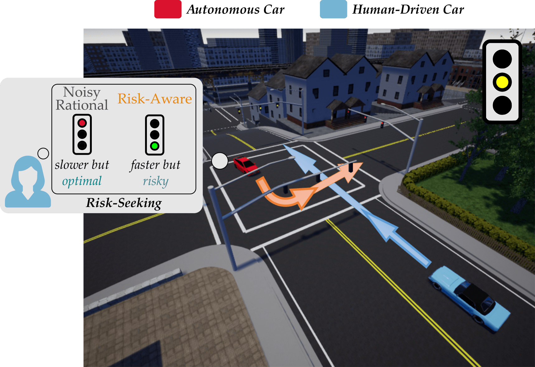
When robots collaborate with humans, they must anticipate how the human will behave for seamless and safe interaction. Consider the scenario shown below, where an autonomous car is waiting at an intersection. The autonomous car (red) wants to make an unprotected left turn, but a human driven car (blue) is approaching in the oncoming lane.
The stoplight has just turned yellow for the human driven car. It is unclear whether the driver will accelerate — and try to make the light — or stop and play it safe. If the autonomous car thinks that the human will stop, it makes sense for the autonomous car to turn right; but if the robot anticipates that the human may try and make the light, it should wait for the human to go! Put another way, the robot needs to correctly anticipate what the human will do. And in order to do that, the robot needs to correctly model the human — i.e., correctly interpret how the human will make their decisions.
Background. Previous work has explored different approaches for robots tomodel humans. One common approach is to assume that humans also act like robots, and make perfectly rational decisions to maximize their utility or reward1. But we know that this isn’t always true: humans often make mistakes or suboptimal decisions, particularly when we don’t have much time to make a decision, or when the decision requires thinking about complex trade-offs. In recognition of this, today’s robots typically anticipate that humans will make noisily rational choices2. A noisily rational human is most likely to choose the best option, but there is also a nonzero chance that this human may act suboptimally, and select an action with lower expected reward. Put another way, this human is usually right, but occasionally they can make mistakes.
What’s Missing? Modeling people as noisily rational makes sense when humans are faced with deterministic decisions. Let’s go back to our driving example, where the autonomous car needs to predict whether or not the human will try to run the light. Here, a deterministic decision occurs when the light will definitely turn red in seconds: the human knows if they will make the light, and can accelerate or decelerate accordingly. But in real world settings, we often do not know exactly what will happen as a consequence of our actions. Instead, we must deal with uncertainty by estimating risk! Returning to our example, imagine that if the human accelerates there is a % chance of making the light and saving commute time, and a % chance of running a red light and getting fined. It makes sense for the human to stop (since decelerating leads to the most reward in expectation), but a risk-seeking driver may still attempt to make the light.
Assuming that humans are rational or noisily rational doesn’t make sense in scenarios with risk and uncertainty. Here we need models that can incorporate the cognitive biases in human decision making, and recognize that it is likely that the human car will try and run the light, even though it is not optimal!
Insight and Contributions. When robots model humans as noisily rational, they miss out on how risk biases human decision-making. Instead, we assert:
To ensure safe and efficient interaction, robots must recognize that people behave suboptimally when risk is involved.
Inspired by work in behavioral economics, we propose using Cumulative Prospect Theory3 as a Risk-Aware model for human-robot interaction. As we’ll show, using the Risk-Aware model is practically useful because it improves safety and efficiency in human-robot collaboration tasks.
Modeling Humans: Noisy Rational vs Risk-Aware
Here we will formalize how we model human decision-making, and then compare the state-of-the-art Noisy Rational human model to our proposed Risk-Aware model.
Notation. We assume a setting where the human needs to select from a discrete set of actions . Taking an action may lead to several possible states, or outcomes. Returning to our driving example, the set of actions is , and choosing to accelerate may lead to making or running the light. Based on the outcome, the human receives some reward — ideally, the human will obtain as much reward as possible. For a given human action , we can express the expected reward across all possible outcomes as:
where is the probability of outcome , and there are possible outcomes. Overall, this equation tells us how valuable the choice is to the human4.
The Rational Model. If the human behaved like a robot — and made perfectly rational decisions — then we might anticipate that the human will choose the action that leads to the highest reward . Let’s use the Boltzmann distribution to write the probability of choosing action , and model the human as always choosing the action with the highest reward:
Our rational model is fairly straightforward: the human always chooses the most likely action. But we know this isn’t the case; humans often make mistakes, have cognitive biases, and select suboptimal options. In fact, Herbert Simon received a Nobel Prize and Turing Award for researching this very trend!
The Noisy Rational Model. We can relax our model so that the human usually chooses the best action:
where is a temperature parameter, commonly referred to as the rationality coefficient. Tuning tells us how frequently the human chooses the best action. When , the human always picks the best action, and when , the human chooses actions uniformly at random.
Uncertainty and Biases. One problem with the Noisy Rational model is that — no matter how we tune — the model never thinks that a suboptimal action is most likely. This is problematic in real-world scenarios because humans exhibit cognitive biases that make it more likely for us to choose suboptimal options! Moving forward, we want to retain the general structure of the Noisy Rational model, while expanding this model to also recognize that there are situations where suboptimal actions are the most likely choices.
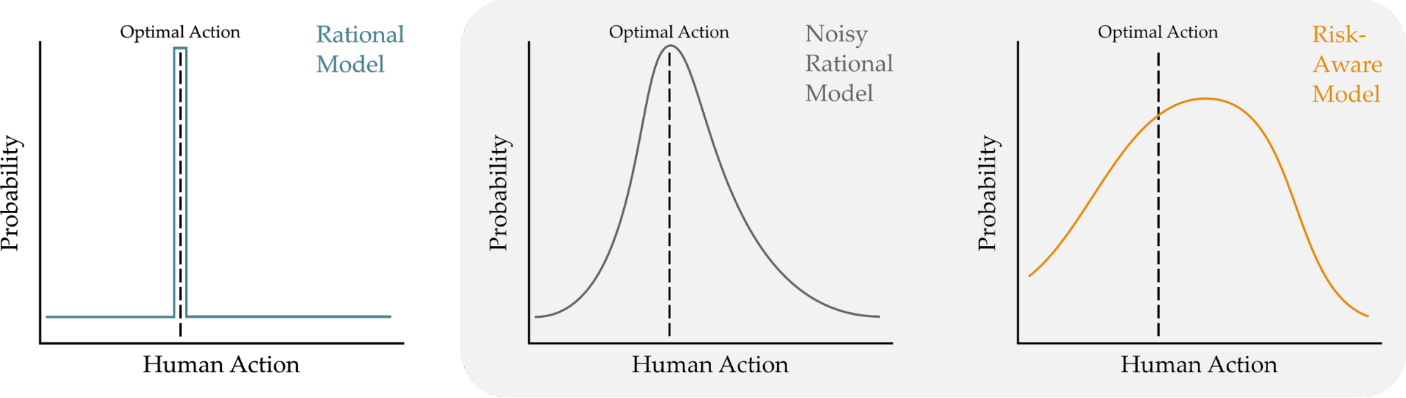
Our Risk-Aware Model. Drawing from behavioral economics, we adopt Cumulative Prospect Theory as a way to incorporate human biases under risk and uncertainty. This model captures both optimal and suboptimal decision-making by transforming the rewards and the probabilities associated with each outcome. We won’t go over all the details here, but we can summarize some of the major changes from the previous models.
-
Transformed rewards. There is often a difference between the true reward associated with a state and the reward the human perceives. For example, humans perceive the differences between large rewards (e.g., million vs. million) as smaller than the differences between low rewards (e.g., vs. ). More formally, if the original reward of outcome is , we will write the human’s transformed reward as .
-
Transformed probabilities. Humans can also exaggerate the likelihood of outcomes when making decisions. Take playing the lottery: even if the probability of winning is almost zero, we buy tickets thinking we have a chance. We capture this in our Cumulative Prospect Theory model, so that if is the true probability of outcome , then is the transformed probability that the human perceives.
With these two transformations in mind, let’s rewrite the expected reward that the human associates with an action:
What’s important here is that the expected reward that the human perceives is different than the real expected reward. This gap between perception and reality allows for the robot to anticipate that humans will choose suboptimal actions:
Comparing our result to the Noisy Rational model, we use the same probability distribution to explain human actions, but now Risk-Aware robots transform both the rewards and probabilities to match known cognitive biases.
Summary. We have outlined two key ways in which we can model how humans make decisions in real-world scenarios. Under the Noisy Rational model, the optimal action is always the most likely human action. By contrast, our Risk-Aware model is able to predict both optimal and suboptimal behavior by non-linearly transforming rewards and probabilities.
Are Risk-Aware Robots Better at Predicting Human Actions?
Now that we’ve established how we are going to model humans, we want to determine whether these models are accurate. More specifically, we will compare our proposed Risk-Aware model to the current state-of-the-art Noisy Rational model. We will stick with our motivating scenario, where an autonomous car is trying to guess whether or not the human driven car will speed through a yellow light.
Autonomous Driving Task. Let’s say that you are the human driver (blue). Your car is a rental, and you are currently on your way to return it. If the light turns red — and you speed through — you will have to pay a fine. But slowing down and stopping at the yellow light will prevent you from returning the rental car on time, which also has an associated late penalty. Would you accelerate (and potentially run the red light) or stop (and return the rental car with a late penalty)?
Experimental Overview. We recruited human drivers, and asked them what action they would choose (accelerate or stop). To better understand what factors affected their decision, we varied the amount of information, time, and risk in the driving scenario:
- Information. We varied how much information the human drivers had about the likelihood of the light turning red. Participants were either given NO information (so that they had to rely on their personal prior), IMPLICIT information (where they got to observe the experiences of previous drivers), or EXPLICIT information (where they knew the exact probability).
- Time. We varied how quickly the human drivers had to make their decision. In TIMED, participants were forced to choose to stop or accelerate in under seconds. In NOT TIMED, the participants could deliberate as long as necessary.
- Risk. Finally, we adjusted the type of uncertainty the human drivers faced when making their decision. In HIGH RISK the light turned red % of the time, so that stopping was the optimal action. By contrast, in LOW RISK the light only turned red in % of trials, so that accelerating became the optimal action.
Results. We measured how frequently the human drivers chose each action across each of these different scenarios. We then explored how well the Noisy Rational and Risk-Averse models captured these action distributions.
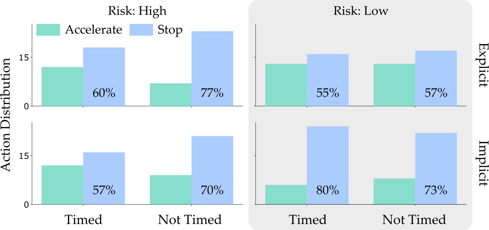
Action Distribution. Across all of our surveyed factors (information, time, and risk), our users preferred to stop at the light. We find that the most interesting comparison is between the High and Low Risk columns. Choosing to stop was the optimal option in the High Risk case (i.e. where the light turns red % of the time) but stopping was actually the suboptimal decision in the Low Risk case when the light rarely turns red. Because humans behaved optimally in some scenarios and suboptimally in others, the autonomous car interacting with these human drivers must be able to anticipate both optimal and suboptimal behavior.
Modeling. Now that we know what the actual human drivers would do, how accurately can we predict these actions? We computed the Noisy Rational and Risk-Aware models that best fit our action distributions. To measure the accuracy of these models, we compared the divergence between the true action distribution and the models’ prediction (lower is better):
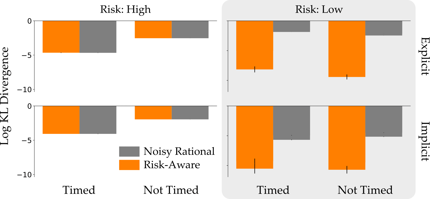
On the left you can see the High Risk case, where humans usually made optimal decisions. Here both models did an equally good job of modeling the human drivers. In the Low Risk case, however, only the Risk Aware model was able to capture the user’s tendency to make suboptimal but safe choices.
Why Risk-Aware is More Accurate. To understand why Risk Aware was able to get both of these scenarios right, let’s look at the human model. More specifically, let’s look at how the Risk-Aware model transformed the probabilities and rewards:
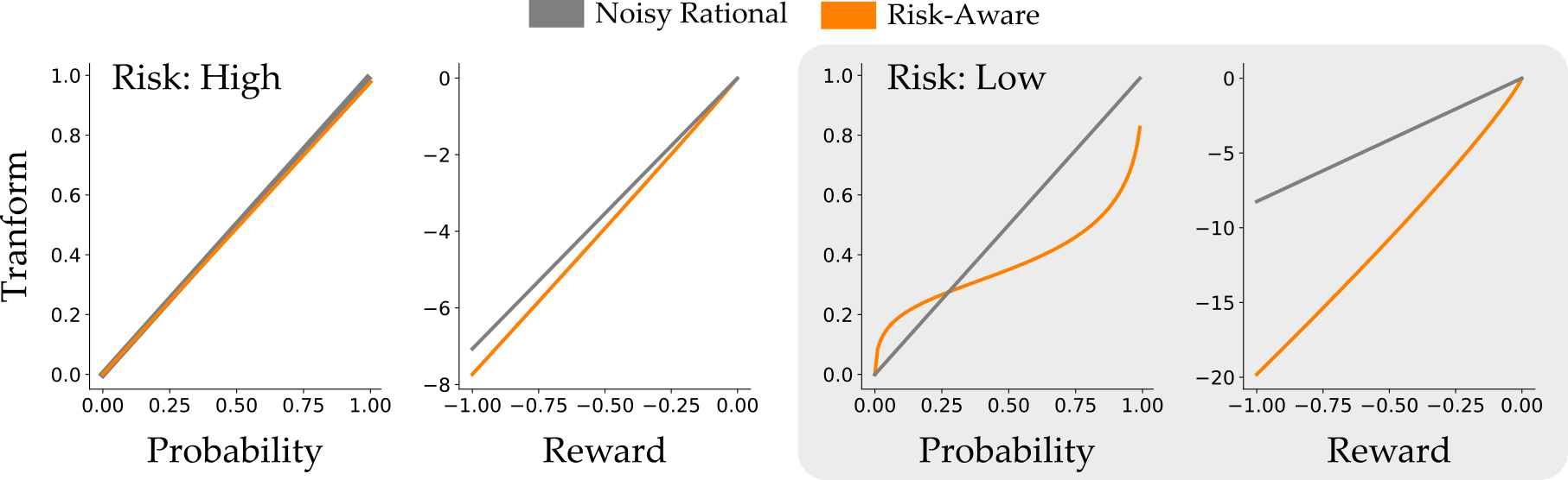
On the left we’re again looking at the High Risk scenario: the Risk-Aware model barely changes the probability and reward here. But when the light rarely turns red in Low Risk, the models diverge! The Risk-Aware model recognizes that human drivers overestimate both the probability that the light will turn red and the penalty for running the light. This enables the Risk-Aware model to explain why human drivers prefer to stop, even though accelerating is the optimal action.
Summary. When testing how human drivers make decisions under uncertainty, we found scenarios where the suboptimal decision was actually the most likely human action. While Noisy Rational models are unable to explain or anticipate these actions, our Risk-Aware model recognized that humans were playing it safe: overestimating the probability of a red light and underestimating the reward for making the light. Accounting for these biases enabled the Risk-Aware model to more accurately anticipate what the human driver would do.
Robots that Plan with Risk-Aware Models
We now know that Risk-Aware models can better predict suboptimal human behavior. But why is this useful? One application would be to leverage these models to improve safety and efficiency in human-robot teams. To test the usefulness of the Risk-Aware model, we performed a user study with a robotic arm, where participants collaborated with the robot to stack cups into a tower.
Collaborative Cup Stacking Task. The collaborative cup stacking task is shown below.
The human and robot are trying to stack all five cups to form a tower. There are two possible tower configurations: an efficient but unstable tower, which is more likely to fall, or an inefficient but stable tower, which requires more robot movement to assemble. Users were awarded points for building the stable tower (which never fell) and for building the unstable tower (which fell % of the time). You can see examples of both types of towers below, with the efficient tower on the left and the stable tower on the right:
If the tower fell over, the human and robot team received no points! Looking at the expected reward, we see that building the efficient but unstable tower is actually the rational choice. But — building on our previous example — we recognize that actual users may prefer to play it safe, and go with the guaranteed success. Indeed, this tendency to avoid risk was demonstrated in our preliminary studies, where % of the time users preferred to make the stable tower!
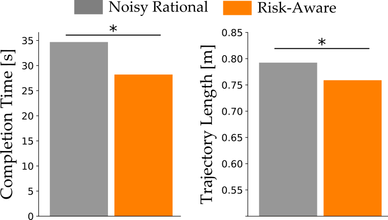
Experimental Overview. Each participant had familiarization trials to practice building towers with the robot. During these trials, users learned about the probabilities of each type of tower collapsing from experience. In half of the familiarization trials, the robot modeled the human with the Noisy Rational model, and in the rest the robot used the Risk-Aware model. After the ten familiarization trials, users built the tower once with the Noisy Rational robot and the Risk-Aware robot. We measured efficiency (completion time) and safety (trajectory length) during collaboration. Because the robot had to replan longer trajectories when it interfered with the human, shorter trajectory lengths indicate safer interactions.
Model Predictions. The robot tried building the tower with two different models of the human: the Noisy Rational baseline and our Risk-Aware model. Planning with these models led the robot to choose two different trajectories:
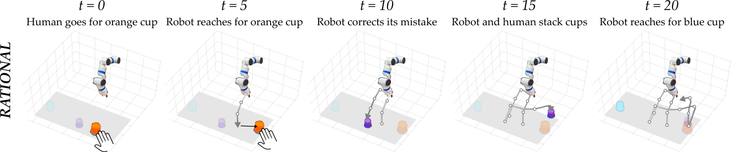
Aggressive but Rational. When the robot is using the Noisy Rational model, it immediately goes for the closer cup, since this behavior is more efficient. Put another way, the robot using the Noisy Rational model incorrectly anticipates that the human wants to make the efficient but unstable tower. This erroneous prediction causes the human and robot to clash, and the robot has to undo its mistake (as you can see in the video above).
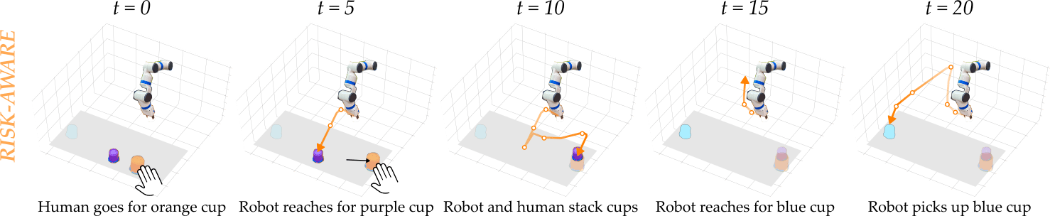
Conservative and Risk-Aware. A Risk-Aware robot gets this prediction right: it correctly anticipates that the human is overly concerned about the tower falling, and starts to build the less efficient but stable tower. Having the right prediction here prevents the human and robot from reaching for the same cup, so that they more seamlessly collaborate during the task!
Results. In our in-person user studies, participants chose to build the stable tower % of the time. The suboptimal choice was more likely — which the Noisy Rational model failed to recognize. By contrast, our Risk-Aware robot was able to anticipate what the human would try to do, and could correctly guess which cup it should pick up. This improved prediction accuracy resulted in human-robot teams that completed the task more efficiently (in less time) and safely (following a shorter trajectory):
We also surveyed users to find their subjective response when working with these different robots. Our questions covered how enjoyable the interaction was (Enjoy), how well the robot understood human behavior (Understood), how accurately the robot predicted which cups they would stack (Predict), and how efficient users perceived the robot to be (Efficient). After they completed the task with both Noisy Rational and Risk-Aware robots, we also asked which type of robot they would rather work with (Prefer) and which robot better anticipated their behavior (Accurate):
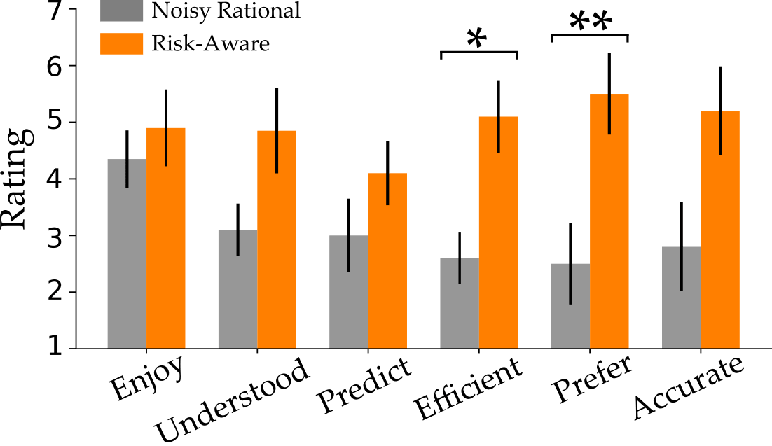
The participants’ responses to our survey are shown above. Each question was on a -point Likert scale, where higher scores indicate agreement. We found that participants preferred the Risk-Aware robot, and thought it was more efficient than the alternative. The other scales favor Risk-Aware, but were not statistically significant.
Summary. Being able to correctly predict that humans will make suboptimal decisions is important for robot planning. We incorporated our Risk-Aware model into a robot working with a human during a collaborative task. This model led to improved safety and efficiency, and people also subjectively perceived the Risk-Aware robot as a better teammate.
Key Takeaways
We explored how we can better model human decision making under risk and uncertainty. Our main insight is that when humans are uncertain, robots should recognize that people behave suboptimally. We extended state-of-the-art prediction models to account for these suboptimal decisions:
- Existing Rational and Noisy Rational models anticipate that the best option is always most likely to be chosen.
- We adopted Cumulative Prospect Theory from behavioral economics, and showed how it can explain and predict suboptimal decisions.
- In both an autonomous driving task and a collaborative block stacking task we found that the Risk-Aware model more accurately predicted human actions.
- Incorporating risk into robot predictions of human actions improves safety and efficiency.
Overall, this work is a step towards robots that can seamlessly anticipate what humans will do and collaborate in interactive settings.
If you have any questions, please contact Minae Kwon at: mnkwon@stanford.edu
Our team of collaborators is shown below!

This blog post is based on the 2020 paper When Humans Aren’t Optimal: Robots that Collaborate with Risk-Aware Humans by Minae Kwon, Erdem Biyik, Aditi Talati, Karan Bhasin, Dylan P. Losey, and Dorsa Sadigh.
For further details on this work, check out the paper on Arxiv.
-
Pieter Abbeel and Andrew Ng, “Apprenticeship learning via inverse reinforcement learning,” ICML 2004. ↩
-
Brian Ziebart et al., “Maximum entropy inverse reinforcement learning,” AAAI 2008. ↩
-
Amos Tversky and Daniel Kahneman, “Advances in prospect theory: Cumulative representation of uncertainty,” Journal of Risk and Uncertainty 1992. ↩
-
In this blog post we will deal with single-decision tasks. The generalization to longer horizon, multi-step games is straightforward using value functions, and you can read more about it in our paper! ↩

Does On-Policy Data Collection Fix Errors in Off-Policy Reinforcement Learning?
Reinforcement learning has seen a great deal of success in solving complex decision making problems ranging from robotics to games to supply chain management to recommender systems. Despite their success, deep reinforcement learning algorithms can be exceptionally difficult to use, due to unstable training, sensitivity to hyperparameters, and generally unpredictable and poorly understood convergence properties. Multiple explanations, and corresponding solutions, have been proposed for improving the stability of such methods, and we have seen good progress over the last few years on these algorithms. In this blog post, we will dive deep into analyzing a central and underexplored reason behind some of the problems with the class of deep RL algorithms based on dynamic programming, which encompass the popular DQN and soft actor-critic (SAC) algorithms – the detrimental connection between data distributions and learned models.