Language Model Pretraining

Language models (LMs), like BERT ¹ and the GPT series ², achieve remarkable performance on many natural language processing (NLP) tasks. They are now the foundation of today’s NLP systems. ³ These models serve important roles in products and tools that we use every day, such as search engines like Google ⁴ and personal assistants like Alexa ⁵.

These LMs are powerful because they can be pretrained via self-supervised learning on massive amounts of text data on the web without the need for labels, after which the pretrained models can be quickly adapted to a wide range of new tasks without much task-specific finetuning. For instance, BERT is pretrained to predict randomly masked words in original text (masked language modeling), e.g. predicting the masked word “dog” from “My __ is fetching the ball”. GPTs are pretrained to predict the next word given a previous sequence of text (causal language modeling), e.g. predicting the next word “ball” from “My dog is fetching the”. In either cases, through pretraining, LMs learn to encode various knowledge from a text corpus that helps to perform downstream applications involving language understanding or generation. In particular, LMs can learn world knowledge (associations between concepts like “dog”, “fetch”, “ball”) from training text where the concepts appear together, and help for knowledge-intensive applications like question answering. ⁶

Challenges.
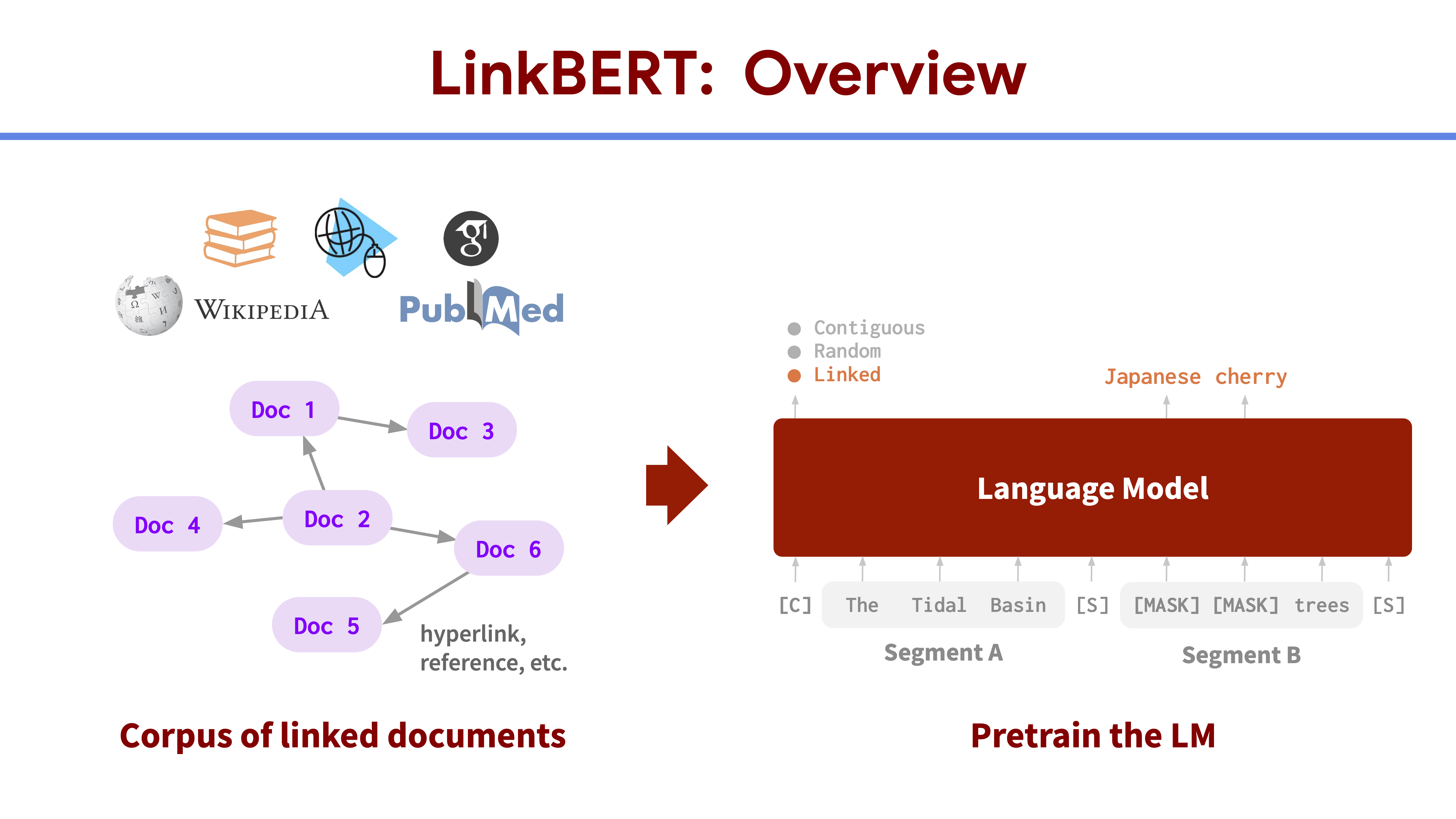
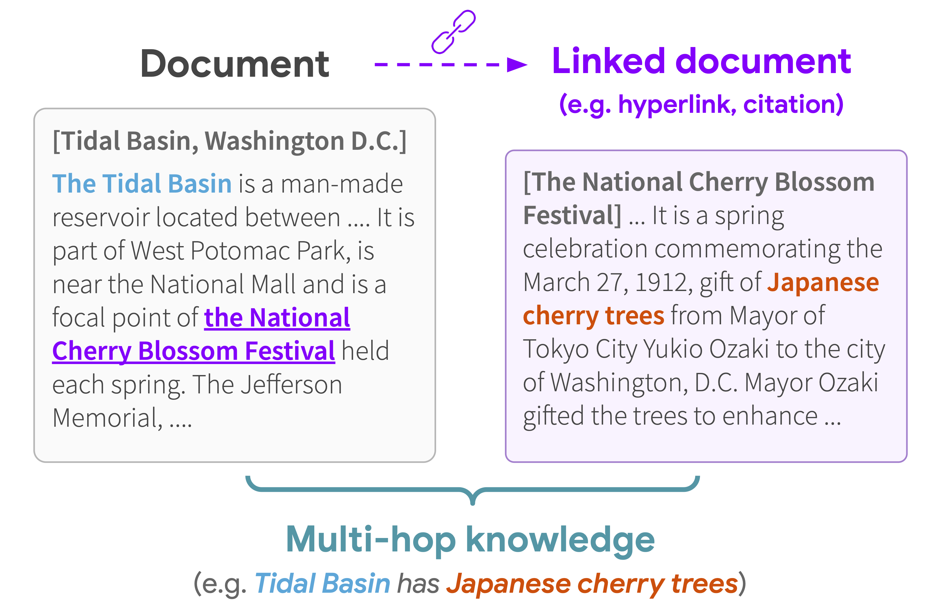
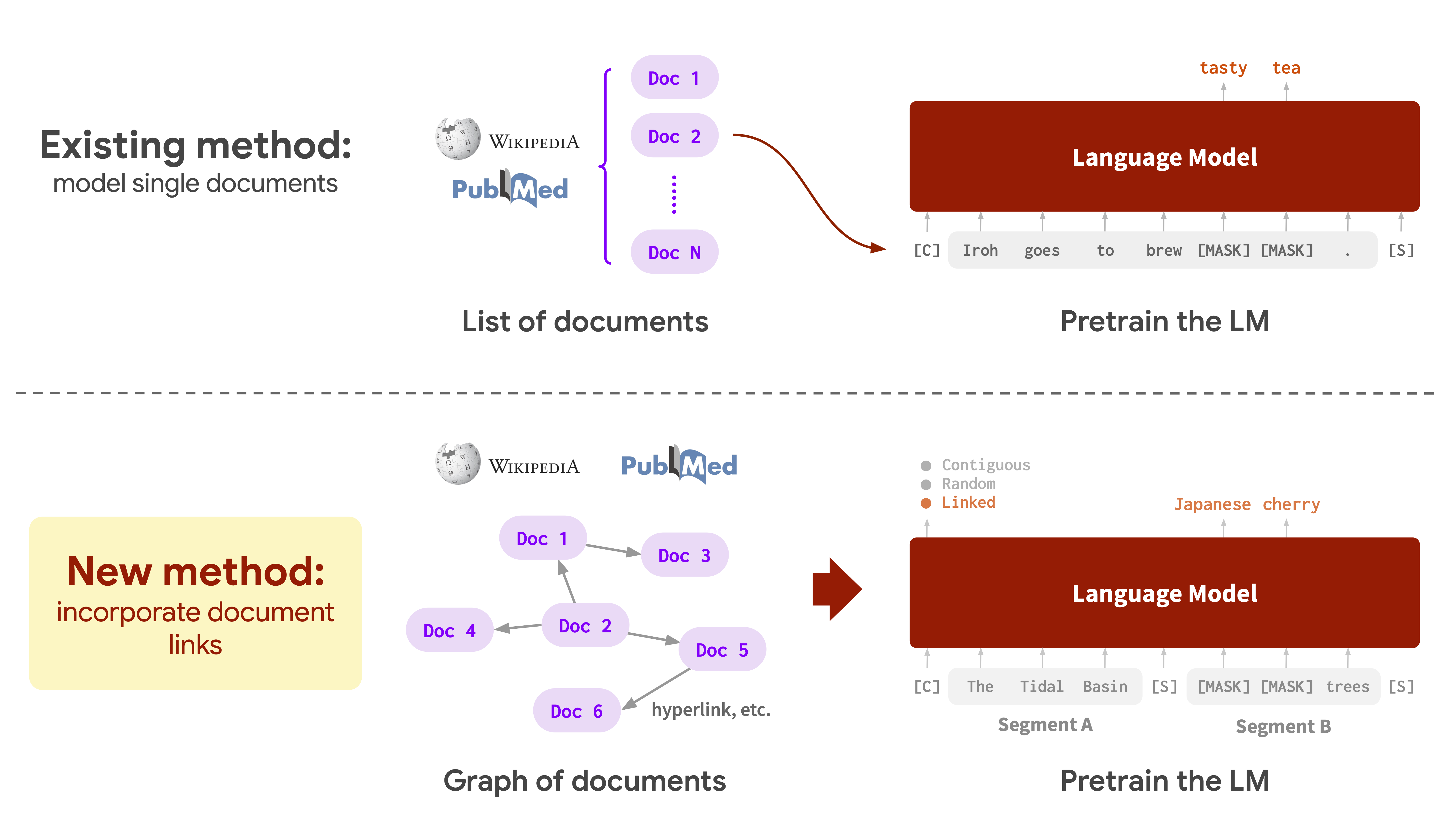
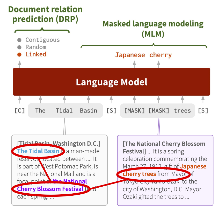
A challenge with most common LM pretraining strategies is that they model a single document at a time. That is, one would split a text corpus into a list of documents and draw training instances for LMs from each document independently. Treating each document independently may pose limitations because documents often have rich dependencies with each other. For instance, text from the web ⁷ or scientific literature ⁸ is often used for LM training, but they all have document links, such as hyperlinks and citation links. Document links are crucial because knowledge can span across multiple documents beyond a single document. As an example, the Wikipedia article “Tidal Basin, Washington D.C.” shown on the left of the figure below describes that the basin hosts “National Cherry Blossom Festival”, and if we jump to the hyperlinked article shown on the right, we see that the festival celebrates “Japanese cherry trees”. Combined, the hyperlink offers new, multi-hop knowledge such as “Tidal Basin has Japanese cherry trees”, which is not available in the original single document alone.

Models that train without these dependencies may fail to capture knowledge or facts that are spread across multiple documents. Learning such multi-hop knowledge in pretraining can be important for various applications including question answering and knowledge discovery (e.g. “What trees can you see at the Tidal Basin?”). Indeed, document links like hyperlinks and citations are ubiquitous and we humans also use them all the time to learn new knowledge and make discoveries. A text corpus is thus not simply a list of documents but a graph of documents with links connecting each other.

In our recent work ⁹ published at ACL 2022, we develop a new pretraining method, LinkBERT, that incorporates such document link information to train language models with more world knowledge.

Approach: LinkBERT

At a high level, LinkBERT consists of three steps: (0) obtaining links between documents to build a document graph from the text corpus, (1) creating link-aware training instances from the graph by placing linked documents together, and finally (2) pretraining the LM with link-aware self-supervised tasks: masked language modeling (MLM) and document relation prediction (DRP).

Document Graph Construction.
Given a text corpus, we link related documents to make a graph so that the links can bring together useful knowledge. Although this graph can be derived in any way, we will focus on using hyperlinks and citation links as they generally have high quality of relevance (i.e. low false-positive rate) and are available ubiquitously at scale. ¹⁰ To make the document graph, we treat each document as a node, and add a directed edge (i, j) if there is a hyperlink from document i to document j.

Link-aware LM Input Creation.
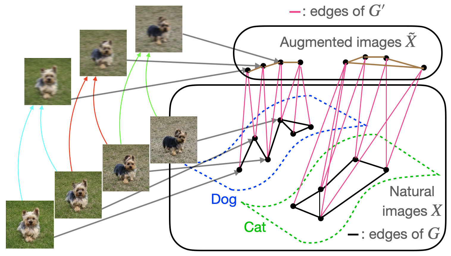
Given the document graph, we then create link-aware inputs that will be fed into our LM. As LMs can learn token dependency effectively if the tokens are shown in the same input instance ¹¹, we want to place linked documents together in the input instance. In this way, the LM can learn multi-hop or multi-document dependencies of concepts as the LM will see training instances where these concepts appear together in the same sequence. To achieve this, we first chunk each document into segments of roughly 256 tokens, which is half of the maximum BERT LM input length. Then, we concatenate two segments (Segment A and B) together as an input sequence for the LM according to the links in the document graph. We have three options for how to choose segments to concatenate together:

• Option 1: contiguous segments. Take two contiguous segments from the same document. This is essentially the same as previous LMs.
• Option 2: random segments. Sample one segment from a random document and sample a second segment from another random document.
• Option 3: linked segments. Sample one segment from a random document and sample a second segment randomly from a document linked to the first document in the document graph.
  The reason we have these three options is to create a training signal for LinkBERT such that the model will learn to recognize relations between text segments. We will explain this in the next paragraph.

Link-aware LM Pretraining.
After creating input instances made up of pairs of segments, the last step is to use these created inputs to train the LM with link-aware self-supervised tasks. We consider the following two tasks:

• Masked language modeling (MLM), which masks some tokens in the input text and then predicts the tokens using the surrounding tokens. This encourages the LM to learn multi-hop knowledge of concepts brought into the same context by document links. For instance, in our running example about Tidal Basin, the LM would be able to learn the multi-hop relations from “Tidal Basin” to “National Cherry Blossom Festival” to “Japanese cherry trees”, as these three concepts will be all presented together in the same training instances.
• Document relation prediction (DRP), which makes the model classify the relation of Segment B to Segment A as to whether the two segments are contiguous, random or linked. This task encourages the LM to learn relevance and dependencies between documents, and also learn bridging concepts such as “National Cherry Blossom Festival” in our running example.

We pretrain the LM with these two objectives jointly.

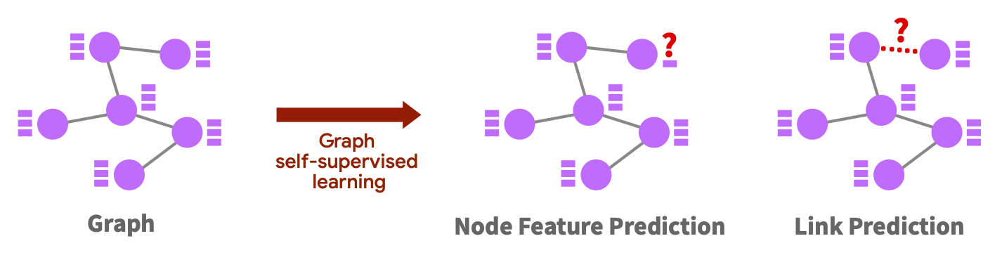
We can also motivate these two pretraining tasks as performing self-supervised learning algorithms on the document graph:

• Node feature prediction ¹², which is to predict masked features of a node using neighbor nodes. This corresponds to MLM, where we predict masked tokens in Segment A using Segment B and vice versa.
• Link prediction ¹³, which is to predict the existence or type of an edge between two nodes. This corresponds to DRP, where we predict if two segments are linked (edge), contiguous (self-loop), or random (no edge).

Let’s use LinkBERT!

We will now see how LinkBERT performs on several downstream natural language processing tasks. We pretrained LinkBERT in two domains:

• General domain: we use Wikipedia as the pretraining corpus, which is the same as previous language models like BERT, except that here we also use the hyperlinks between Wikipedia articles.
• Biomedical domain: we use PubMed as the pretraining corpus, which is the same as previous biomedical language models like PubmedBERT ¹⁴, except that here we also use the citation links between PubMed articles.

LinkBERT improves previous BERT models on many applications.
We evaluated the pretrained LinkBERT models on diverse downstream tasks in each domain:

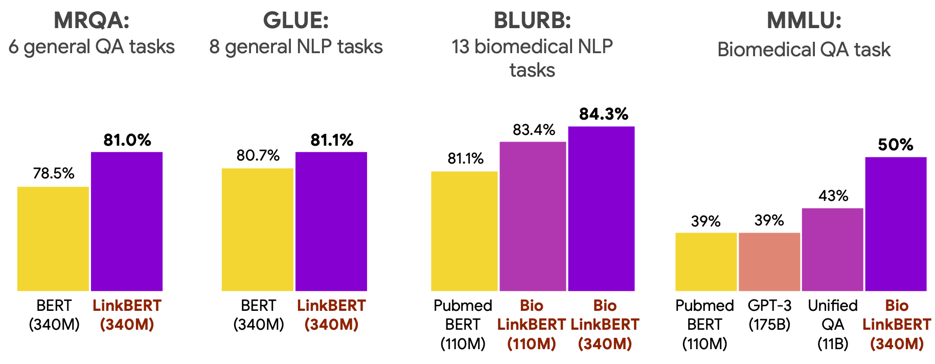
• General question answering (MRQA) and general NLP (GLUE) benchmarks
• Biomedical NLP (BLURB) and biomedical question answering (MedQA, MMLU) benchmarks.

LinkBERT improves the baseline language models pretrained without document links (i.e. BERT and PubmedBERT) consistently across tasks and domains. The gain for the biomedical domain is especially large, likely because scientific literature has crucial dependencies with each other via citation links, which are captured by LinkBERT. The biomedical LinkBERT, which we call BioLinkBERT, achieves new state-of-the-art performance on the BLURB, MedQA and MMLU benchmarks.

Effective for multi-hop reasoning.
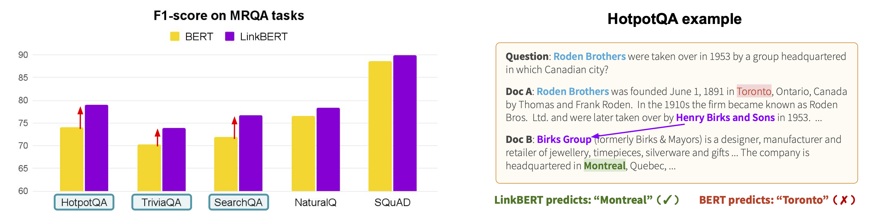
LinkBERT exhibits several interesting strengths. The first strength is multi-hop reasoning. Within the MRQA benchmarks, there are several tasks that involve multi-hop reasoning such as HotpotQA and triviaQA, and we find that LinkBERT provides large improvements for BERT on those tasks. As an example, the figure below shows an example from HotpotQA. Answering the given question needs 2-hop reasoning because we need to know what organization took over Roden Brothers in 1953 (the first document), and then we need to know where that organization was headquartered (the second document). BERT tends to simply predict a location name that appears in the same document as the one about Roden Brothers (“Toronto”), but LinkBERT is able to correctly connect information across the two documents to predict the answer (“Montreal”). The intuition is that because LinkBERT brings together multiple related concepts/documents into the same input instances during pretraining, it helps the model to reason with multiple concepts/documents in downstream tasks.

Effective for document relation understanding.
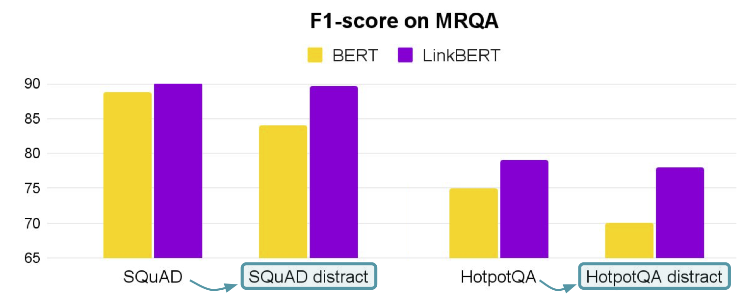
Another strength of LinkBERT is that it can better model the relationships between multiple documents. For instance, in open-domain QA, a model must identify an answer from multiple retrieved documents, where many of the documents are likely noisy or otherwise unrelated to the question. ¹⁵ To simulate this, we added distracting documents to the original MRQA tasks such as SQuAD and HotpotQA. We find that LinkBERT is robust to irrelevant documents and maintains the QA accuracy, while BERT incurs a performance drop in this setup. Our intuition is that the Document Relation Prediction task used in pretraining helps recognizing document relevance in downstream tasks.

Effective for few-shot and data-efficient QA.
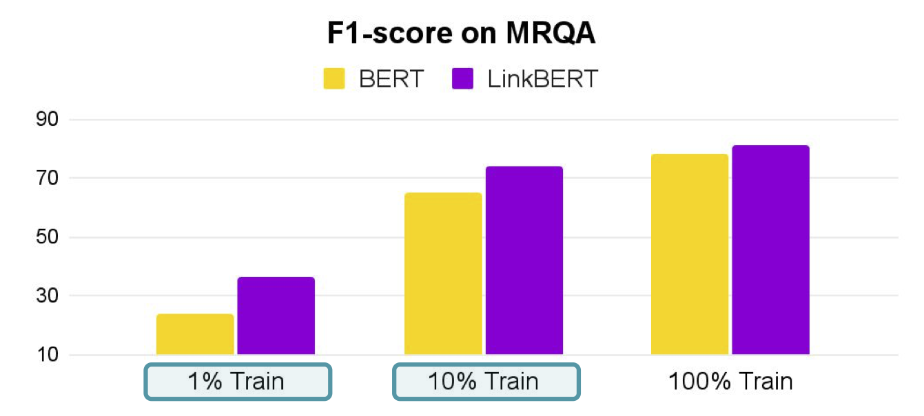
The third strength is few-shot and data-efficient QA. For each QA dataset, we tried finetuning LinkBERT or BERT with only 10% or 1% of the available training data. We find that LinkBERT provides large improvements for BERT on these low-resource paradigms. This finding suggests that LinkBERT has internalized more knowledge than BERT during pretraining, and supports the original intuition that document links can bring in new, useful knowledge for LMs.

Use LinkBERT for your own applications

LinkBERT can be used easily as a drop-in replacement for BERT. The pretrained LinkBERT models (LinkBERT and BioLinkBERT) are available on HuggingFace, and you can load them by

from transformers import AutoTokenizer, AutoModel
tokenizer = AutoTokenizer.from_pretrained('michiyasunaga/LinkBERT-large')
model = AutoModel.from_pretrained('michiyasunaga/LinkBERT-large')
inputs = tokenizer("Hello, my dog is cute", return_tensors="pt")
outputs = model(**inputs)

from transformers import AutoTokenizer, AutoModel
tokenizer = AutoTokenizer.from_pretrained('michiyasunaga/BioLinkBERT-large')
model = AutoModel.from_pretrained('michiyasunaga/BioLinkBERT-large')
inputs = tokenizer("Sunitinib is a tyrosine kinase inhibitor", return_tensors="pt")
outputs = model(**inputs)

To use LinkBERT for downstream applications such as question answering and text classification, you can use the finetuning scripts provided at https://github.com/michiyasunaga/LinkBERT, or simply replace the BERT model path with LinkBERT in your favorite BERT finetuning scripts.

Summary

We introduced LinkBERT, a new pretraining method that leverages document links such as hyperlinks and citations to train a knowledgeable language model (LM). Specifically, we place linked documents in the same LM input sequence, and train the LM with two joint self-supervised tasks: masked language modeling and document relation prediction.

LinkBERT can be used as a drop-in replacement for BERT. In addition to improving performance for general language understanding tasks (e.g. text classification), LinkBERT better captures document or concept relations, and is effective for multi-hop reasoning and cross-document understanding. LinkBERT also internalizes more world knowledge and is effective for knowledge-intensive tasks, such as few-shot question answering.

We release the pretrained LinkBERT models. We hope they can be helpful for your projects and research, especially knowledge or reasoning-intensive applications. Finally, we think that LinkBERT opens up many exciting future projects, such as generalizing to GPT or sequence-to-sequence ¹⁶ style language models to perform document link-aware text generation, and generalizing the notion of document links to other modalities, e.g., incorporating source code dependency links in the training of language models for code ¹⁷.

This blog post is based on the paper:

• LinkBERT: Pretraining Language Models with Document Links. Michihiro Yasunaga, Jure Leskovec and Percy Liang. ACL 2022. The models, code, data are available on GitHub and HuggingFace.

If you have questions, please feel free to email us.

• Michihiro Yasunaga: myasu@cs.stanford.edu

Acknowledgments

Many thanks to the members of the Stanford P-Lambda group, SNAP group and NLP group for their valuable feedback. Many thanks to Jacob Schreiber and Michael Zhang for edits on this blog post.

Read More

The 60th Annual Meeting of the Association for Computational Linguistics (ACL) 2022 is taking place May 22nd – May 27th. We’re excited to share all the work from SAIL that’s being presented, and you’ll find links to papers, videos and blogs below. Feel free to reach out to the contact authors directly to learn more about the work that’s happening at Stanford!

List of Accepted Papers

LinkBERT: Pretraining Language Models with Document Links

Authors: Michihiro Yasunaga, Jure Leskovec*, Percy Liang*

Contact: myasu@cs.stanford.edu

Links: Paper | Website

Keywords: language model, pretraining, knowledge, hyperlink, bionlp

When classifying grammatical role, BERT doesn’t care about word order… except when it matters

Authors: Isabel Papadimitriou, Richard Futrell, Kyle Mahowald

Contact: isabelvp@stanford.edu

Links: Paper

Keywords: large language models, analysis, word order, order invariance, grammatical role, syntax, semantics

Problems with Cosine as a Measure of Embedding Similarity for High Frequency Words

Authors: Kaitlyn Zhou, Kawin Ethayarajh, Dallas Card, Dan Jurafsky

Contact: katezhou@stanford.edu

Keywords: cosine similarity, training data frequency, model analysis

Faithful or Extractive? On Mitigating the Faithfulness-Abstractiveness Trade-off in Abstractive Summarization

Authors: Faisal Ladhak, Esin Durmus, He He, Claire Cardie, Kathleen McKeown

Contact: esdurmus@stanford.edu

Links: Paper

Keywords: text summarization, text generation, evaluation, faithfulness

Spurious Correlations in Reference-Free Evaluation of Text Generation

Authors: Esin Durmus, Faisal Ladhak, Tatsunori Hashimoto

Contact: esdurmus@stanford.edu

Links: Paper

Keywords: text summarization, text generation, dialogue generation, evaluation, metrics,

TABi: Type-Aware Bi-Encoders for Open-Domain Entity Retrieval

Authors: Megan Leszczynski, Daniel Y. Fu, Mayee F. Chen, Christopher Ré

Contact: mleszczy@stanford.edu

Links: Paper | Blog Post | Website

Keywords: entity retrieval, contrastive learning, bi-encoders

A Few-Shot Semantic Parser for Wizard-of-Oz Dialogues with the Precise ThingTalk Representation

Authors: Giovanni Campagna, Sina J. Semnani, Ryan Kearns, Lucas Jun Koba Sato, Silei Xu, Monica S. Lam

Contact: gcampagn@cs.stanford.edu

Venue: Findings of ACL

Links: Paper | Website

Keywords: dialogue agents, task-oriented dialogues, data synthesis

Richer Countries and Richer Representations

Authors: Kaitlyn Zhou, Kawin Ethayarajh, Dan Jurafsky

Contact: katezhou@stanford.edu

Venue: Findings of ACL

Keywords: representational harms, model analysis, geographic entities

Modular Domain Adaptation

Authors: Junshen K. Chen, Dallas Card, Dan Jurafsky

Contact: dalc@umich.edu

Venue: Findings of ACL

Links: Paper | Blog Post | Website

Keywords: domain adaptation, computational social science, text classification, lexicons, sentiment

Shared Autonomy for Robotic Manipulation with Language Corrections

Authors: Siddharth Karamcheti*, Raj Palleti*, Yuchen Cui, Percy Liang, Dorsa Sadigh

Contact: skaramcheti@cs.stanford.edu

Venue: ACL LNLS workshop

Links: Paper

Keywords: human-robot interaction, online language corrections, language supervision

Read More

The International Conference on Learning Representations (ICLR) 2022 is being hosted virtually from April 25th – April 29th. We’re excited to share all the work from SAIL that’s being presented, and you’ll find links to papers, videos and blogs below. Feel free to reach out to the contact authors directly to learn more about the work that’s happening at Stanford!

List of Accepted Papers

Autonomous Reinforcement Learning: Formalism and Benchmarking

Authors: Archit Sharma*, Kelvin Xu*, Nikhil Sardana, Abhishek Gupta, Karol Hausman, Sergey Levine, Chelsea Finn

Contact: architsh@stanford.edu

Links: Paper | Website

Keywords: reinforcement learning, continual learning, reset-free reinforcement learning

MetaShift: A Dataset of Datasets for Evaluating Contextual Distribution Shifts and Training Conflicts

Authors: Weixin Liang, James Zou

Contact: wxliang@stanford.edu

Links: Paper | Video | Website

Keywords: benchmark dataset, distribution shift, out-of-domain generalization

An Explanation of In-context Learning as Implicit Bayesian Inference

Authors: Sang Michael Xie, Aditi Raghunathan, Percy Liang, Tengyu Ma

Contact: xie@cs.stanford.edu

Links: Paper | Video

Keywords: gpt-3, in-context learning, pretraining, few-shot learning

GreaseLM: Graph REASoning Enhanced Language Models for Question Answering

Authors: Xikun Zhang, Antoine Bosselut, Michihiro Yasunaga, Hongyu Ren, Percy Liang, Christopher D. Manning, Jure Leskovec

Contact: xikunz2@cs.stanford.edu

Award nominations: Spotlight

Links: Paper | Website

Keywords: knowledge graph, question answering, language model, commonsense reasoning, graph neural networks, biomedical qa

Fast Model Editing at Scale

Authors: Eric Mitchell, Charles Lin, Antoine Bosselut, Chelsea Finn, Christopher D. Manning

Contact: eric.mitchell@cs.stanford.edu

Links: Paper | Website

Keywords: model editing; meta-learning; language models; continual learning; temporal generalization

Vision-Based Manipulators Need to Also See from Their Hands

Authors: Kyle Hsu, Moo Jin Kim, Rafael Rafailov, Jiajun Wu, Chelsea Finn

Contact: kylehsu@cs.stanford.edu

Award nominations: Oral Presentation

Links: Paper | Website

Keywords: reinforcement learning, observation space, out-of-distribution generalization, visuomotor control, robotics, manipulation

IFR-Explore: Learning Inter-object Functional Relationships in 3D Indoor Scenes

Authors: Qi Li*, Kaichun Mo*, Yanchao Yang, Hang Zhao, Leonidas J. Guibas

Contact: kaichun@cs.stanford.edu

Links: Paper

Keywords: embodied ai, 3d scene graph, interactive perception

VAT-Mart: Learning Visual Action Trajectory Proposals for Manipulating 3D ARTiculated Objects

Authors: Ruihai Wu*, Yan Zhao*, Kaichun Mo*, Zizheng Guo, Yian Wang, Tianhao Wu, Qingnan Fan, Xuelin Chen, Leonidas J. Guibas, Hao Dong

Contact: kaichun@cs.stanford.edu

Links: Paper | Video | Website

Keywords: visual affordance learning, robotic manipulation, 3d perception, interactive perception

Language modeling via stochastic processes

Authors: Rose E Wang

Contact: rewang@stanford.edu

Award nominations: Oral Presentation

Links: Paper | Video | Website

Keywords: contrastive learning, language modeling, stochastic processes

MetaMorph: Learning Universal Controllers with Transformers

Authors: Agrim Gupta, Linxi Fan, Surya Ganguli, Li Fei-Fei

Contact: agrim@stanford.edu

Links: Paper | Video | Website

Keywords: rl, modular robots, transformers

Fine-Tuning can Distort Pretrained Features and Underperform Out-of-Distribution

Authors: Ananya Kumar

Contact: ananya@cs.stanford.edu

Award nominations: Oral Presentation

Links: Paper

Keywords: fine-tuning theory, transfer learning theory, fine-tuning, distribution shift, implicit regularization

An Experimental Design Perspective on Model-Based Reinforcement Learning

Authors: Viraj Mehta, Biswajit Paria, Jeff Schneider, Stefano Ermon, Willie Neiswanger

Contact: virajm@cs.cmu.edu, neiswanger@cs.stanford.edu

Links: Paper

Keywords: reinforcement learning, model-based reinforcement learning, mbrl, bayesian optimal experimental design, boed, bax

Domino: Discovering Systematic Errors with Cross-Modal Embeddings

Authors: Sabri Eyuboglu*, Maya Varma*, Khaled Saab*, Jean-Benoit Delbrouck, Christopher Lee-Messer, Jared Dunnmon, James Zou, Christopher Ré

Contact: {eyuboglu,mvarma2,ksaab}@stanford.edu

Award nominations: Oral Presentation

Links: Paper | Blog Post | Website

Keywords: robustness, subgroup analysis, error analysis, multimodal, slice discovery

Pixelated Butterfly: Simple and Efficient Sparse training for Neural Network Models

Authors: Tri Dao, Beidi Chen, Kaizhao Liang, Jiaming Yang, Zhao Song, Atri Rudra, Christopher Ré

Contact: trid@stanford.edu

Award nominations: Spotlight

Links: Paper | Blog Post

Keywords: sparse training, butterfly matrices

Hindsight: Posterior-guided training of retrievers for improved open-ended generation

Authors: Ashwin Paranjape, Omar Khattab, Christopher Potts, Matei Zaharia, Christopher D Manning

Contact: ashwinp@cs.stanford.edu

Links: Paper

Keywords: retrieval, generation, retrieval-augmented generation, open-ended generation, informative conversations, free-form qa, posterior distribution, elbo

Unsupervised Discovery of Object Radiance Fields

Authors: Hong-Xing Yu, Leonidas J. Guibas, Jiajun Wu

Contact: koven@cs.stanford.edu

Links: Paper | Video | Website

Keywords: object-centric representation, unsupervised, 3d object discovery

Efficiently Modeling Long Sequences with Structured State Spaces

Authors: Albert Gu, Karan Goel, Christopher Ré

Contact: albertgu@stanford.edu

Award nominations: Outstanding Paper Honorable Mention

Links: Paper | Blog Post | Video

Keywords: hippo

How many degrees of freedom do we need to train deep networks: a loss landscape perspective

Authors: Brett W. Larsen, Stanislav Fort, Nic Becker, Surya Ganguli

Contact: bwlarsen@stanford.edu

Links: Paper

Keywords: loss landscape, high-dimensional geometry, random hyperplanes, optimization

How did the Model Change? Efficiently Assessing Machine Learning API Shifts

Authors: Lingjiao Chen, Matei Zaharia, James Zou

Contact: lingjiao@stanford.edu

Links: Paper | Website

Keywords: mlaas, performance shifts, ml systems

We look forward to seeing you at ICLR 2022!

Read More

Discovering systematic errors with cross-modal embeddings

In this blog post, we introduce Domino, a new approach for discovering systematic errors made by machine learning models. We also discuss a framework for quantitatively evaluating methods like Domino.

Links:
📄 Paper (ICLR 2022)
🌍 Longer Walkthrough
💻 GitHub
📘 Docs
📒 Google Colab

Machine learning models that achieve high overall accuracy often make systematic errors on coherent slices of validation data.

What is a slice? A slice is a set of data samples that share a common characteristic. As an example, in large image datasets, photos of vintage cars comprise a slice (i.e. all images in the slice share a common subject). The term slice has a number of synonyms that you might be more familiar with (e.g. subgroup, subpopulation, stratum). These terms are largely interchangeable, but we’ll stick with “slice” throughout this post. We say that a model underperforms on a slice if performance on the data samples in the slice is significantly worse than its overall performance.

The search for underperforming slices is a critical, but often overlooked, part of model evaluation. When practitioners are aware of the slices on which their models underperform, they can make more informed decisions around model deployment. This is particularly important in safety-critical settings like medicine: a diagnostic model that underperforms on younger patients should likely not be deployed at a pediatric hospital. Slice awareness can also help practitioners debug and improve models: after an underperforming slice is identified, we can improve model robustness by either updating the training dataset or using robust optimization techniques (e.g. Sohoni et al., 2020; Sagawa et al., 2020).

Deploying models that underperform on critical data slices may have significant safety or fairness consequences. For example, models trained to detect collapsed lungs in chest X-rays have been shown to make predictions based on the presence of chest drains, a device typically used during treatment (Oakden-Rayner, 2019). As a result, these models often fail to detect collapsed lung in images without chest drains, a critical data slice where false negative predictions could be life-threatening.

However, in practice, some underperforming slices are hard to find. The examples in these “hidden” data slices are tied together by a concept not annotated in metadata or easily extracted from unstructured inputs (e.g. images, video, time-series data). Returning to our example from earlier, many chest X-ray datasets do not provide metadata indicating which patients’ images show chest tubes, making it difficult to evaluate performance on the slice. This raises the following question: How can we automatically identify data slices on which our model underperforms?

In this blog post, we discuss our recent exploration of this question. We introduce Domino, a novel method for identifying and describing underperforming slices. We also discuss an evaluation framework for rigorously evaluating our method across diverse slice types, tasks, and datasets.

What is slice discovery?

Slice discovery is the task of mining unstructured input data (e.g. images, videos, audio) for semantically meaningful subgroups on which a model performs poorly. We refer to automated techniques that mine input data for semantically meaningful slices as slice discovery methods (SDM). Given a labeled validation dataset and a trained classifier, an SDM computes a set of slicing functions that partition the dataset into slices. This process is illustrated below.

In order to be broadly useful across diverse settings, an ideal SDM should satisfy the following desiderata:

1. Identified slices should contain examples on which the model underperforms, or has a high error rate.
2. Identified slices should contain examples that are coherent, or align closely with a human-understandable concept.

This second desideratum is particularly hard to achieve: existing evaluations have shown that discovered slices often do not align with concepts understandable to a domain expert. Further, even if slices do align well with concepts, it may be difficult for humans to identify the commonality.

Domino: Slice discovery with cross-modal embeddings

In our work, we introduce Domino, a slice discovery method designed to identify coherent, underperforming data slices (i.e. groups of similar validation data points on which the model makes errors). It leverages a powerful class of recently-developed cross-modal representation learning approaches, which yield semantically-meaningful representations by embedding images and text in the same latent space. We demonstrate that using cross-modal representations both improves slice coherence and enables Domino to generate natural language descriptions for identified slices!

Domino follows a three-step procedure illustrated in the figure above:

1. Embed: Domino encodes the validation images alongside text in a shared embedding space using a cross-modal encoder. In many domains, such encoders are publicly available (e.g. CLIP for natural images, VideoCLIP for natural videos, ConVIRT for medical images, and CLASP for amino acid sequences).
2. Slice: Using an error-aware mixture model, Domino identifies regions in the embedding space with a high concentration of errors.
3. Describe: Finally, to help practitioners understand the commonalities among the examples in each slice, Domino generates natural language descriptions of the slices. To do so, it leverages the cross-modal embeddings computed in Step 1, surfacing the text nearest to the slice in embedding space.

We now use Domino to audit a popular off-the-shelf classifier: a ResNet18 pretrained on ImageNet. Specifically, we interrogate the model’s ability to detect cars, exploring whether there are any interesting slices on which the model underperforms. In the figure below we show a couple of the slices that Domino discovered. The gray boxes show the natural language descriptions of the two slices produced by Domino, the $X$ row shows the top six images predicted by domino to be in the slice, the $Y$ row shows the ground truth label assigned to the image, and the $hat{Y}$ row shows the ResNet18’s predicted probability for the “car” class. Note that although we only include six images here, the complete slice includes dozens of images.

From these slices, we might hypothesize that the model struggles to recognize photos of cars taken from the inside and photos of racecars. Both of these slices describe rare subclasses of the target class. Depending on the intended use case for the model, we may want to add more training examples to boost performance in these slices. For example, Waymo (an autonomous vehicle company) may not care much whether the model misses photos of car interiors, but ESPN (a broadcaster with the television rights for Formula 1) would care a lot if the model couldn’t recognize race cars! Clearly, it’s important to practitioners that discovered slices map onto coherent concepts.

Evaluating slice discovery methods

In designing Domino, we were inspired by a number of really exciting slice discovery methods that were recently proposed. These include The Spotlight (D’Eon et al. 2022), GEORGE (Sohoni et al. 2020), and MultiAccuracy Boost (Kim et al. 2018). These methods all have (1) an embed step and (2) a slice step, like Domino, but use different embeddings and slicing algorithms. In our experiments, we evaluate SDMs along these two axes, ablating both the choice of embedding and the slicing algorithm. Notably, these methods do not include a (3) describe step, and generally require users to manually inspect examples and identify common attributes.

SDMs like Domino have traditionally been evaluated qualitatively, due to a lack of a simple quantitative approach. Typically, in these evaluations, the SDM is applied to a few different models and identified slices are visualized. Practitioners can then inspect the slices and judge whether the slices “make sense.” However, these qualitative evaluations are subjective and do not scale beyond more than a few settings. Moreover, they cannot tell us if the SDM has missed an important, coherent slice.

Ideally, we’d like to estimate the failure rate of an SDM: how often it fails to identify a coherent slice on which the model underperforms. Estimating this failure rate is very challenging because we don’t typically know the full set of slices on which a model underperforms. How could we possibly know if the SDM is missing any?

To solve this problem, we trained 1,235 deep classifiers that were specifically constrained to underperform on pre-defined slices. We did this across three domains: natural images, medical images and medical time-series. Our approach involved (1) obtaining a dataset with some annotated slices (e.g. a dataset with interesting annotated attributes, like CelebA or MIMIC-CXR), and (2) manipulating the dataset such that, with high probability, a model trained on it would exhibit poor performance on one or more of the annotated slices (e.g. by subsampling the dataset to induce a spurious correlation between the label and a metadata field).

Using this evaluation framework, we were able to evaluate Domino quantitatively. We find that Domino accurately identifies 36% of the 1,235 slices in our framework. Further, the natural language description of the generated slice exactly matches the name of the slice in 35% of settings.

We were also able to compare SDMs and run ablation studies evaluating specific SDM design choices. Two key findings emerged from these experiments:

1. Cross-modal embeddings improve SDM performance. We found that the choice of representation matters – a lot! Slice discovery methods based on cross-modal embeddings outperform those based on a single modality by at least 9 percentage-points in precision-at-10. When compared with using the activations of the trained model, the gap grows to 15 percentage points. This finding is of particular interest given that classifier activations are a popular embedding choice in existing SDMs.
2. Modeling both the prediction and class label enables accurate slice discovery. Good embeddings alone do not suffice – the choice of algorithm for actually extracting the underperforming slices from the embedding space, is significant as well. We find that a simple mixture model that jointly models the embeddings, labels and predictions enables a 105% improvement over the next best slicing algorithm. We hypothesize that this is because this algorithm is unique in modeling the class labels and the model’s predictions as separate variables, which leads to slices which are “pure” in their error type (false positive vs. false negative).

However, there’s still a long way to go: slice discovery is a challenging task, and Domino, the best performing method in our experiments, still fails to recover over 60% of coherent slices. We see a number of exciting avenues for future work that could begin to close this gap.

• We suspect that improvements in the embeddings that power slice discovery will be driven by large cross modal datasets, so work in dataset curation and management could help push the needle.

• In this blog post, we described slice discovery as a fully automated process, while, in the future, we expect that effective slice discovery systems will be highly interactive: practitioners will be able to quickly explore slices and provide feedback. Forager, a system for rapid data exploration, is an exciting step in this direction.

We are really excited to continue working on this important problem and to collaborate with others as we seek to develop more reliable slice discovery methods. To facilitate this process, we are releasing 984 models and their associated slices as part of dcbench, a suite of data centric benchmarks. This will allow others to reproduce our results and also develop new slice discovery methods. Additionally, we are also releasing domino, a Python package containing implementations of popular slice discovery methods. If you’ve developed a new slice discovery method and would like us to add it to the library please reach out!

Read More

[Summary] tl;dr:
A tremendous amount of effort has been poured into training AI algorithms to competitively play games that computers have traditionally had trouble with, such as the retro games published by Atari, Go, DotA, and StarCraft II. The practical machine learning knowledge accumulated in developing these algorithms has paved the way for people to now routinely train game-playing AI agents for many games. Following this line of work, we focus on a specific category of games – those developed by students as part of a programming assignment. Can the same algorithms that master Atari games help us grade these game assignments? In our recent NeurIPS 2021 paper, we illustrate the challenges in treating interactive coding assignment grading as game playing and introduce the Play to Grade Challenge.

Introduction

Massive Online Coding Education has reached striking success over the past decade. Fast internet speed, improved UI design, code editors that are embedded in a browser window allow educational platforms such as Code.org to build a diverse set of courses tailored towards students of different coding experiences and interest levels (for example, Code.org offers “Star War-themed coding challenge,” and “Elsa/Frozen themed for-loop writing”). As a non-profit organization, Code.org claims to have reached over 60 million learners across the world ¹. Such organizations typically provide a variety of carefully constructed teaching materials such as videos and programming challenges.

A challenge faced by these platforms is that of grading assignments. It is well known that grading is critical to student learning ², in part because it motivates students to complete their assignments. Sometimes manual grading can be feasible in small settings, or automated grading used in simple settings such as when assignments are multiple choice or adopt a fill-in-the-blink modular coding structure. Unfortunately, many of the most exciting assignments, such as developing games or interactive apps, are also much more difficult to automatically evaluate. For such assignments, human teachers are currently needed to provide feedback and grading. This requirement, and the corresponding difficulty with scaling up manual grading, is one of the biggest obstacles of online coding education. Without automated grading systems, students who lack additional teacher resources cannot get useful feedback to help them learn and advance through the materials provided.

Programming a game that is playable is exciting for students who are learning to code. Code.org provides many game development assignments in their curriculum. In these assignments, students write JavaScript programs in a code editor embedded in the web browser. Game assignments are great for teachers to examine student’s progress as well: students not only need to grasp basic concepts like if-conditionals and for-loops but use these concepts to write the physical rules of the game world — calculate the trajectories of objects, resolve inelastic collision of two objects, and keep track of game states. To deal with all of these complexities, students need to use abstraction (functions/class) to encapsulate each functionality in order to manage this complex set of logic.

Automated grading on the code text alone can be an incredibly hard challenge, even for introductory level computer science assignments. As examples, two solutions which are only slightly different in text can have very different behaviors, and two solutions that are written in very different ways can have the same behaviors. As such, some models that people develop for grading code can be as complex as those used to understand paragraphs of natural language. But, sometimes, grading code can be even more difficult than grading an essay because coding submissions can be in different programming languages. In this situation, one must not only develop a program that can understand many programming languages, but guard against the potential that the grader is more accurate for some languages than others. A Finally, these programs must be able to generalize to new assignments because correct grading is just as necessary for the first student working on an assignment as the millionth – the collect-data, train, deploy cycle is not quite suitable in this context. We don’t have the luxury of collecting a massive amount of labeled dataset to train a fully supervised learning algorithm for each and every assignment.

In a recent paper, we circumvent these challenges by developing a method that grades assignments by playing them, without needing to look at the source code at all. Despite this different approach, our method still manages to provide scalable feedback that potentially can be deployed in a massively-online setting.

The Play to Grade Challenge

Our solution to these problems is to ignore the code text entirely and to grade an assignment by having a grading algorithm play it. We represent the underlying game of each program submission as a Markov Decision Process (MDP), which defines a state space, action space, reward function, and transition dynamics. By running each student’s program, we can build the MDP directly without needing to read or understand the underlying code. You can read more about the MDP framework here: ³.

Since all student programs are written for the same assignment, these programs should generate MDP with a lot of commonalities, such as shared state and action space. After playing the game and fully constructing the MDP for an assignment, all we need is to compare the MDP specified by the student’s program (student MDP) to the teacher’s solution (reference MDP) and determine if these two MDPs are the same. What sets this challenge apart from any other reinforcement learning problems is the fact that a classification needs to be made at the end of this agent’s interaction with this MDP — the decision of whether the MDP is the same as the reference MDP or not.

In order to solve this challenge, we present an algorithm with two components: an agent that plays the game and can reliably reach bug states, and a classifier that can recognize bug states (i.e., provide the probability of the observed state being a bug). Both components are necessary for accurate grading: an agent that reaches all states but cannot determine if any represents bugs is just as bad as a perfect classifier paired with an agent that is bad at taking actions which might cause bugs. Imagine a non-optimal agent that never catches the ball (in the example above) – this agent will never be able to test if the wall, or paddle, or goal does not behave correctly.

An ideal agent needs to produce differential trajectories, i.e., sequences of actions that can be used to differentiate two MDPs, and must contain at least one bug-triggering state if the trajectory is produced from the incorrect MDP. Therefore, we need both a correct MDP and a few incorrect MDPs to teach the agent and the classifier. These incorrect MDPs are incorrect solutions that can either be provided by the teacher, or come from manually grading a few student programs to find common issues. Although having to manually label incorrect MDPs is an annoyance, we show that the total amount of effort is generally significantly lower than grading each assignment: in fact, we show that for the task we solve in the paper, you only need 5 incorrect MDPs to reach a decent performance (see the appendix section of our paper).

Recognizing Bugs from Scratch

Here are three incorrect programs and what they look like when played. Each incorrect program behaves differently from the correct program:

• One program’s wall does not allow the ball to bounce on it.
• Another program’s goal post does not let the ball go through.
• The last program spawns 2 new balls whenever the ball bounces on the wall.

A challenge with building differential trajectories is that one must know which state is a bug triggering state. Previous works ⁴⁵⁶ have made the strong assumption that one would automatically know when they encountered a bug, potentially because they expect the game program to crash after encountering a bug. Because of this assumption, they focus their efforts on building pure-exploration agents that try to visit as many states as possible. However, in reality, bugs can be difficult to identify and do not all cause the game to crash. For example, a ball that is supposed to bounce off of a wall is now piercing through it and flying off into oblivion. These types of behavioral anomalies motivate the use of a predictive model that can take in the current game state and determine whether it is anomalous or not.

Unfortunately, training a model to predict if a state is a bug state is non-trivial. This is because, although we have labels for some MDPs, these labels are not on the state-level (i.e., not all states in an incorrect MDP are bug states). Put another way, our labels can tell us when a bug has been encountered but cannot tell us what specific action caused the bug. The determination of whether bugs exist in a program can be framed as a chicken-and-egg problem where, if bug states could be unambiguously determined one would only need to explore the state space, and if the exploration was optimal one would only need to figure out how to determine if the current state exhibited a bug.

Collaborative Reinforcement Learning

Fortunately, these types of problems can generally be solved through the expectation-maximization framework, which involves an intimate collaboration between the neural network classifier and the reinforcement learning agent. We propose collaborative reinforcement learning, an expectation-maximization approach, where we use a random agent to produce a dataset of trajectories from the correct and incorrect MDP to teach the classifier. Then the classifier would assign a score to each state indicating how much the classifier believes the state is a bug-triggering state. We use this score as reward and train the agent to reach these states as often as possible for a new dataset of trajectories to train the classifier.

After using the RL agent to interact with the MDP to produce trajectories, we can try out different ways to learn a classifier that can classify a state as a bug or not (a binary label). Choosing the right label is important because this label will become the reward function for the agent, so it can learn to reach bug states more efficiently. However, we only know if the MDP (the submitted code) is correct or broken, but we don’t have labels for the underlying states. Learning state-level labels becomes a challenge!

We tested out several types of classifiers: (1) a noisy classifier that classifies all states in a broken MDP as broken, (2) a Gaussian Mixture Model that treats all states independently, (3) a Variational Autoencoder that also treats all states independently but directly models non-linear interactions among the features, or (4) an LSTM that jointly models the teacher program as an MDP (HoareLSTM) and an LSTM that models the student program as an MDP (Contrastive HoareLSTM) – with a distance function that compares the two MDPs, borrowing distance notions from literature in MDP homomorphism⁷⁸⁹¹⁰.

In this toy environment, the agent drives a car on a 2D plane. Whenever the agent drives the car into the outer rim of this area (space between the boundary and red dotted line), a bug will cause the car to get stuck (Leftmost panel in Figure 5). Being stuck means the car’s physical movement is altered, resulting in back-and-forth movement around the same location. The bug classifier needs to recognize the resulting states (position and velocity) of the car being “stuck”, by correctly outputting a binary label (bug) for these states.

In this setting, there is only one type of bug. Most classifiers do well when the agent only drives a straight line (single-direction agent). However, when the agent randomly samples actions at each state, simpler classifiers can no longer differentiate between bug and non-bug states with high accuracy.

We can increase the difficulty of this setting to see if collaborative training can make the agent operate in the environment with an intention to trigger bugs. In this toy environment, now the bugs will only be triggered in red boxes (Leftmost panel in Figure 6 below). We can see that with only one round of collaborative training (“CT Round 1”), the performances of ALL classifiers are improved, including weaker classifiers. This is understandable, as the agent learns to gradually collect better datasets to train classifiers – and higher quality datasets lead to stronger classifiers. For example, variational auto-encoder started only with 32% precision, but it increased to 74.8% precision after 2 rounds of collaborative training.

We can also visualize how the collaborative training quickly allows the agent to learn to explore states that most-likely contain bugs by visualizing the trajectories (see figure below). Initially the agent just explores the space uniformly (blue curves), but after one round of collaborative training (CT), it learns to focus on visiting the potential bug areas (regions marked by red boxes) (red curves).

Grading Bounce

Next, we returned to the motivating example for this type of approach: grading real student submissions. With help from Code.org, we are able to verify the algorithm’s performance on a massive amount of unlabeled, ungraded student submissions. The game Bounce, from Code.org’s Course3 for students in 4th and 5th grade, provides a real-life dataset of what variations of different bugs and behaviors in student programs should look like. The dataset is compiled of 453,211 students who made an attempt on this assignment. In total, this dataset consists of 711,274 programs.

We train our agent and classifier on 10 broken programs that we wrote without looking at any of the student’s submissions. The 10 programs contain bugs that we “guess” to be most likely to occur, and we use them to train 10 agents that learn to reach bug states in these 10 programs. This means that in our training dataset, we have 1 correct program and 10 broken programs. Even with only 11 labeled programs, our agent and classifier can get 99.5% precision at identifying a bug program and 93.4-94% accuracy overall – the agent is able to trigger most of the bugs and the classifier recognizes the bug states using only 10 broken programs. Though for other games, especially more complicated games, the number of training programs will vary. We strongly believe the number is still in magnitude smaller than training supervised code-as-text algorithms. This demonstration shows the promise of reformulating code assignment grading as the Play to Grade.

What is Next?

We started this project by making the argument that sometimes it is far easier to grade a complex coding assignment not by looking at the code text but by playing it. Using Bounce, we demonstrated that in the simple task of identifying if a program has a bug or not (a binary task, nonetheless), we are able to achieve striking accuracy with only 11 labeled programs. We provide a simulator and all of the student’s programs on this Github repo.

Multi-label Bounce

One promising direction for future work is to expand beyond pass/fail binary feedback, and actually identify which bug is in the student’s program and provide that information. Our Bounce dataset enables this by providing multi-error labels, as shown in the table below. The multi-error label setting was not solved by our current algorithm and remains an open challenge!

More than One Correct Solution

Oftentimes, students create solutions that are creative. Creative solutions are different, but not wrong. For example, students can change the texture pattern of the ball or paddle; or they can make the paddle move much faster. How to set the boundary between “being creative” and “being wrong”? This is not a discussion that happens often in AI, but is of huge importance in education. Though we didn’t use the Bounce dataset to focus on the problem of understanding creativity, our work can still use distance measures to set a “tolerance threshold” to account for creativity.

For Educators

We are interested in collecting a suite of interactive coding assignments and creating a dataset for future researchers to work on this problem. Feel free to reach out to us and let us know what you would consider as important in grading and giving students feedback on their coding assignments!

Conclusion

Providing automated feedback for coding is an important area of research in computational education, and an important area for building fully autonomous coding education pipeline (that can generate coding assignment, grade assignment, and teach interactively). Providing a generalizable algorithm that can play interactive student programs in order to give feedback is an important problem for education and an exciting intellectual challenge for the reinforcement learning community. In this work, we introduce the challenge and a dataset, set up the MDP distance framework that is highly data efficient, algorithms that achieve high accuracy, and demonstrate this is a promising direction of applying machine learning to assist education.

This blog post is based on the following paper:

• “Play to Grade: Testing Coding Games as Classifying Markov Decision Process.” Allen Nie, Emma Brunskill, and Chris Piech. Advances in Neural Information Processing Systems 34 (2021). Link

Acknowledgements

Many thanks to Emma Brunskill, Chris Piech for their guidance on the project. Many thanks to Mike Wu, Ali Malik, Yunsung Kim, Lisa Yan, Tong Mu, and Henry Zhu for their discussion and feedback. Special thanks to code.org, and Baker Franke, for many years of collaboration and generously providing the research community with data. Thanks to Stanford Hoffman-Yee Human Centered AI grant for supporting AI in education. Thanks for the numerous rounds of edits from Megha Srivastava and Jacob Schreiber.

Read More

Labels for large-scale datasets are expensive to curate, so leveraging abundant unlabeled data before fine-tuning them on the smaller, labeled, data sets is an important and promising direction for pre-training machine learning models. One popular and successful approach for developing pre-trained models is contrastive learning, (He et al., 2019, Chen et al., 2020). Contrastive learning is a powerful class of self-supervised visual representation learning methods that learn feature extractors by (1) minimizing the distance between the representations of positive pairs, or samples that are similar in some sense, and (2) maximizing the distance between representations of negative pairs, or samples that are different in some sense. Contrastive learning can be applied to unlabeled images by having positive pairs contain augmentations of the same image and negative pairs contain augmentations of different images.

In this blog post, we will propose a theoretical framework for understanding the success of this contrastive learning approach. Our theory motivates a novel contrastive loss with theoretical guarantees for downstream linear-probe performance. Our experiments suggest that representations learned by minimizing this objective achieve comparable performance to state-of-the-art methods.

Augmentation graph for self-supervised learning

The key idea behind our work is the idea of a population augmentation graph, which also appeared in our previous blog post where we analyzed self-training. As a reminder, this graph is built such that the nodes represent all possible augmentations of all data points in the population distribution and the edges connect nodes that are derived from the same natural image. Further, the edges are weighted to be the probability that the two augmented images are augmentations of the same underlying image, given the set of augmentation functions being used. Some augmentation methods, like cropping, produce images that could only come from the same underlying image. However, others, such as Gaussian blurring, technically connect all images to each other, albeit mostly with very small probabilities. Because there are a potentially infinite number of augmentations, this graph is more of a theoretical idea we will use to describe our idea rather than an actual graph that we construct. The figure below gives a visualization of the graph, where augmented images of French bulldogs are connected in the graph.

We have two simple intuitions about the graph that suggests it contains information generally useful for a pre-trained computer vision model.
First, very few high-probability edges exist between any two images, especially if they have different semantic content. For instance, consider two pictures of the same dogs in different poses. Even though the semantic content is the same, there is almost zero chance that one could produce one image from the other using augmentation methods like Gaussian blur. This probability is reduced further when considering two images that don’t even share the same objects, such as one image of a dog outside and another image of a cruise ship in the ocean. Rather, the only high-probability connections are augmented images with similar objects in similar orientations or poses.
Second, images with similar content (e.g, dog images of the same breed) can be connected to each other via a path of interpolating images. The figure above visualizes this intuition, where (x_1) and (x_2) are two augmented images of French bulldogs that aren’t obtained from the same natural image (hence no high-probability edge between them). However, since the augmentation graph is a theoretical construct that is defined on the population data which contains all possible dog images, there must exist a path of interpolating French bulldog images (as shown in Figure 1) where every consecutive two images are directly connected by a reasonably high-probability edge. As a result, this sequence forms a path connecting (x_1) and (x_2).

Graph partitioning via spectral decomposition

Consider an ideal world where we can partition the augmentation graph into multiple disconnected subgraphs. From the intuition above, each subgraph contains images that can be easily interpolated into each other, and so likely depicts the same underlying concept or objects in its images. This motivates us to design self-supervised algorithms that can map nodes within the same subgraph to similar representations.
Assume we have access to the population data distribution and hence the whole augmentation graph. A successful algorithm for graph partitioning is spectral clustering (Shi & Malik 2000, Ng et al. 2002), which uses spectral graph theory tools to discover the connected components in a graph. We’ll describe spectral clustering in more detail here, and then interpret contrastive learning as an effective, parametric way to implement spectral clustering on the large augmentation graph.
Let X denote the vertex set of the graph, and for the ease of exposition assume ( |X| = N). ((N) can also be infinite or exponential.) Let (Ain mathbb{R}^{Ntimes N}) be the adjacency matrix which contains edge weights (w_{xx’}) as its entries. For every node (x), let (w_x=sum_{x’in X} w_{xx’}) be the sum of weights of edges connected to x (which can be thought of as the degree of the vertex (x)). We call the matrix (L=I-text{diag}(w_x^{-1/2})cdot A cdot text{diag}(w_x^{-1/2})) the Laplacian matrix of the graph.
Spectral clustering begins with eigendecomposition of the Laplacian matrix. Let (u_1, u_2, cdots, u_{k}) be the (N)-dimensional eigenvectors that correspond to the smallest (k) eigenvalues. If we write these vectors as columns of a matrix (F in mathbb{R}^{Ntimes k}), every row (denoted as (v_1, v_2, cdots, v_N in mathbb{R}^{k})) would correspond to a single node in the graph. We can then obtain a (k)-way partition of the graph by running (k)-means on these (N) vectors.

It’s worth noting that we cannot directly run spectral clustering on the population augmentation graph, since its eigendecomposition step requires knowing the entire graph (i.e., all the data in the population), whereas in reality we only have a sampled dataset. However, the intuition behind spectral clustering is still valuable: the smallest eigenvectors of the Laplacian matrix should provide pretty good representations of the data.

Contrastive learning as spectral clustering

We can use these intuitions about spectral clustering to design a contrastive learning algorithm. Specifically, because we don’t have access to the true population augmentation graph, we instead define (f_theta) which is a neural network that takes in an example and outputs the eigenvector representation of the example. Put another way, our goal is to compute the matrix (F) that contains the eigenvectors as columns, and use its rows as the representations. We aim to learn (f_theta) such that (f_theta(x)) is the row of matrix (F) corresponding to example (x). Given the high expressivity of neural nets, we assume that such a (theta) exists.

It turns out that this feature can be learned by minimizing the following “matrix factorization loss”:
(min_{F_theta}L(F_theta) triangleq left| (I-L) – F_theta F_theta^top right|_F^2 =sum_{i, j} left(frac{w_{x_ix_j}}{sqrt{w_{x_i}}sqrt{w_{x_j}}} – f_theta(x_i)^top f_theta(x_j)right)^2)
where (F_thetainmathbb{R}^{Ntimes k}) is the matrix containing (f_theta(x_i)) as its (i)-th row. According to the Eckart–Young–Mirsky theorem, any minimizer of this loss contains the largest eigenvectors of (I-L) (hence the smallest eigenvectors of (L)) as its columns(up to scaling). As a result, at the minimizer, (f_theta) recovers the smallest eigenvectors.
We expand the above loss, and arrive at a formula that (somewhat surprisingly) resembles a contrastive loss:
(begin{aligned} min_{theta} L(f_theta) &= text{const} -2sum_{i, j}frac{w_{x_ix_j}}{sqrt{w_{x_i}}sqrt{w_{x_j}}}f_theta(x_i)^top f_theta(x_j) + sum_{i, j}left(f_theta(x_i)^top f_theta(x_j)right)^2 \
&= text{const} -2mathbb{E}_{x,x^+}frac{f_theta(x)^top}{sqrt{w_x}}frac{f_theta(x^+)}{sqrt{w_{x^+}}} + mathbb{E}_{x,x’}left(frac{f_theta(x)^top}{sqrt{w_x}}frac{f_theta(x’)}{sqrt{w_{x’}}}right)^2
end{aligned})
where ((x, x^+)) is a random positive pair and ((x, x’)) is a random negative pair. In the second line, we are using the fact that (w_{x_ix_j}) and (w_{x_i}w_{x_j}) are the probability densities of ((x_i, x_j)) being a positive and negative pair, respectively, to replace the sums by expectations.
Ignoring the constant term and the scalings (sqrt{w_x}) (which do not influence linear separability of the learned representations), we get the following contrastive loss objective
(min_{theta} L_{text{scl}}(f_theta) = -2mathbb{E}_{x,x^+} left[f_theta(x)^top f_theta(x^+)right] + mathbb{E}_{x,x’}left[left(f_theta(x)^top f_theta(x’)right)^2right])
which we call spectral contrastive loss. The minimizer of this objective would correspond to the smallest eigenvectors of the Laplacian matrix with some data-wise positive scaling.
In summary, the above analysis shows that, when minimizing a special variant of contrastive loss (i.e., spectral contrastive loss), the learned features correspond to the eigenvectors of the Laplacian matrix of the population augmentation graph.

Empirically, features learned by training spectral contrastive loss can match strong baselines such as SimCLR and SimSiam. The above table shows the linear probe accuracy with 100-epoch pre-training on ImageNet. More discussions about the empirical performance of this loss can be found in the experiments section of our paper.

Why does this method produce good representations?

We now turn to the question we began with: why are the representations learned by contrastive loss useful for downstream computer vision tasks? We study the downstream accuracy of the representation with the “linear probe” protocol (Chen et al. 2020), where an additional linear model is trained on the representation to predict the labels for a downstream classification task.
As discussed above, the representations learned by the spectral contrastive loss are the rows (with data-wise positive scaling) of a matrix where the columns are the smallest eigenvectors of the Laplacian matrix. Since the scaling doesn’t change the linear prediction, it suffices to consider the rows of the eigenvector matrix as representations.
The usefulness of this representation in classification tasks can be demonstrated by the following didactic example: consider a augmentation graph (G) with three completely disconnected components that correspond to three classes, and the downstream task is to classify one component (e.g., set ({x_1, x_2, x_3}) versus the rest).

The figure above shows the smallest eigenvectors of the Laplacian, where the blank entries are 0. It’s easy to see that here rows of the eigenvector matrix exactly correspond to indicators of different components in the graph, and hence the representations of nodes from different connected subgraphs are clearly linearly separable. For instance, if we use the sign of (f(x)^top b) as the predictor where vector (binmathbb{R}^{k}) is set to be (e_1), we can perfectly classify whether a node belongs to set ({x_1, x_2, x_3}) or not.
The same intuition holds in a broader setting where the graph isn’t regular, the components aren’t necessarily disconnected, and the downstream task has more than two classes. In summary, the contrastive learned representation can linearly predict any set of nearly disconnected components with high accuracy, which is captured by the following theorem:
Theorem (informal): Assume the population augmentation graph contains (k) approximately disconnected components, where each component corresponds to a downstream class. Let the feature map (f: Xrightarrow mathbb{R}^k) be the minimizer of the population spectral contrastive loss. Then, there exists a linear head on top of (f) that achieves small downstream classification error.
The formal version of this theorem can be found in our paper.

Conclusion

Our theory suggests that self-supervised learning can learn quite powerful and diverse features that are suitable for a large set of downstream tasks. To see this, consider a situation where there are a large number of disconnected subgraphs in the augmentation graph, the downstream task can be an arbitrary way of grouping these subgraphs into a small number of classes (each class can correspond to many subgraphs, .e.g., the “dog” class may contain many subgraphs corresponding to different breeds of dogs).
Due to the abundance of unlabeled data in practice, generalization in the traditional sense (i.e., studying population loss vs. empirical loss) is no longer the main challenge to understanding self-supervised learning. Instead, a good understanding of the population pretraining loss and its connection with the downstream tasks becomes essential. As a result, proper modeling of the pretraining data becomes key to the theoretical analysis. We hope that our theoretical framework, which characterizes properties of the data via the augmentation graph, can facilitate a better understanding of unsupervised algorithms in deep learning and can inspire new practical loss functions and algorithms.
This blog post was based on our NeurIPS 2021 paper Provable Guarantees for Self-Supervised Deep Learning with Spectral Contrastive Loss.

Read More

Deep models require a lot of training examples, but labeled data is difficult to obtain. This motivates an important line of research on leveraging unlabeled data, which is often more readily available. For example, large quantities of unlabeled image data can be obtained by crawling the web, whereas labeled datasets such as ImageNet require expensive labeling procedures. In recent empirical developments, models trained with unlabeled data have begun to approach fully-supervised performance (e.g., Chen et al., 2020, Sohn et al., 2020).

This series of blog posts will discuss our theoretical work which seeks to analyze recent empirical methods which use unlabeled data. In this first post, we’ll analyze self-training, which is a very impactful algorithmic paradigm for semi-supervised learning and domain adaptation. In Part 2, we will use related theoretical ideas to analyze self-supervised contrastive learning algorithms, which have been very effective for unsupervised representation learning.

Background: self-training

We will first provide a basic overview of self-training algorithms, which are the main focus of this blog post. The core idea is to use some pre-existing classifier (F_{pl}) (referred to as the “pseudo-labeler”) to make predictions (referred to as “pseudo-labels”) on a large unlabeled dataset, and then retrain a new model with the pseudo-labels. For example, in semi-supervised learning, the pseudo-labeler is obtained from training on a small labeled dataset, and is then used to predict pseudo-labels on a larger unlabeled dataset. A new classifier (F) is then retrained from scratch to fit the pseudo-labels, using additional regularization. In practice, (F) will often be more accurate than the original pseudo-labeler (F_{pl}) (Lee 2013). The self-training procedure is depicted below.

It is quite surprising that self-training can work so well in practice, given that we retrain on our own predictions, i.e. the pseudo-labels, but not the true labels. In the rest of this blogpost, we’ll share our theoretical analysis explaining why this is the case, showing that retraining in self-training provably improves accuracy compared to the original pseudo-labeler.

Our theoretical analysis focuses on pseudo-label-based self-training, but there are also other variants. For example, entropy minimization, which essentially trains on changing pseudo-labels produced by (F), rather than fixed pseudo-labels from (F_{pl}), can also be interpreted as self-training. Related analysis techniques apply to these algorithms (Cai et al. ‘21).

The importance of regularization for self-training

Before discussing core parts of our theory, we’ll first set up the analysis by demonstrating that regularization during the retraining phase is necessary for self-training to work well.

Let’s consider the retraining step of the self-training algorithm described above. Suppose we minimize the cross-entropy loss to fit the pseudo-labels, as is the case for deep networks. It’s possible to drive the unregularized cross-entropy loss to 0 by scaling up the predictions of (F_{pl}) to infinity. As depicted in Figure 2 below, this means that the retraining step won’t achieve any improvement over (F_{pl}) because the decision boundary will not change. This suggests that regularization might be necessary to have in our analysis if self-training is to lead to provable improvements over the pseudo-labeler.

Empirically, one technique which leads to substantial improvements after the retraining step is to encourage the classifier to have consistent predictions on neighboring pairs of examples. We refer to such methods as forms of input consistency regularization. In the literature, there are various ways to define “neighboring pairs”, for example, examples close in (ell_2) distance (Miyato et al., 2017, Shu et al., 2018), or examples which are different strong data augmentations of the same image (Xie et al., 2019, Berthelot et al., 2019, Xie et al., 2019, Sohn et al., 2020). Strong data augmentation, which applies stronger alterations to the input image than traditionally used in supervised learning, is also very useful for self-supervised contrastive learning, which we will analyze in the follow-up blog post. Our theoretical analysis considers a regularizer which is inspired by empirical work on input consistency regularization.

Key formulations for theoretical analysis

From the discussion above, it’s clear that in order to understand why self-training helps, we need a principled way to think about the regularizer for self-training. Input consistency regularization is effective in practice, but how do we abstract it so that the analysis is tractable? Furthermore, what properties of the data does the input consistency regularizer leverage in order to be effective? In the next section we’ll introduce the augmentation graph, a key concept that allows us to cleanly resolve both challenges. Building upon the augmentation graph, subsequent sections will formally introduce the regularizer and assumptions on the data.

Augmentation graph on the population data

We introduce the augmentation graph on the population data, a key concept which allows us to formalize the input consistency regularizer and motivates natural assumptions on the data distribution.

Intuitively, the augmentation graph is a graph with data points as vertices with the property that semantically similar data points will be connected by sequences of edges. We will consider the bipartite graph (G’) displayed in Figure 3 below, whose vertex set consists of all natural images (X) as well as the set (tilde{X}) of augmented versions of images in (X). The graph contains an edge (in pink) between (x in X) and (tilde{x} in tilde{X}) if (tilde{x}) is obtained by applying data augmentation to (x).

The analysis will be slightly simpler if we work with the graph (G) obtained by collapsing (G’) onto the vertex set (X). Edges of (G) are shown in black and connect vertices (x_1, x_2 in X) which share a common neighbor in (G’). Natural images (x_1, x_2 in X) are neighbors in (G) if and only if they share a common neighbor in (G’). In our next post on self-supervised contrastive learning algorithms, we will also consider the graph obtained by collapsing (G’) onto (tilde{X}), whose edges are shown in brown in the figure above.

For simplicity, we only consider unweighted graphs and focus on data augmentations which blur the image with small (ell_2)-bounded noise, although the augmentation graph can be constructed based on arbitrary types of data augmentation. The figure above shows examples of neighboring images in (G), with paired colored arrows pointing to their common augmentations in (tilde{X}). Note that by following edges in (G), it is possible to traverse a path between two rather different images, even though neighboring images in (G) are very similar and must have small (ell_2) distance from each other. An important point to stress is that (G) is a graph on the population data, not just the training set – this distinction is crucial for the type of assumptions we will make about (G).

Formalizing the regularizer

Now that we’ve defined the augmentation graph, let’s see how this concept helps us formulate our analysis. First, the augmentation graph motivates the following natural abstraction for the input consistency regularizer:

In this definition, the neighborhood (N(x)) is the set of all (x’) such that (x) and (x’) are connected by an edge in the augmentation graph. The final population self-training objective which we will analyze is a sum of the regularizer and loss in fitting the pseudo-label and is closely related to empirically successful objectives such as in (Xie et al., 2019, Sohn et al., 2020).

Assumptions on the data

We will now perform a thought experiment to see why the regularizer is useful, and in doing so motivate two key assumptions for our analysis. Let’s consider an idealized case where the classifier has perfect input consistency, i.e., (R(F, x) = 0) for all (x). If the data satisfies an appropriate structure, enforcing perfect input consistency can be very advantageous, as visualized below.

The figure above demonstrates that if the dog class is connected in (G), enforcing perfect input consistency will ensure that the classifier makes the same prediction on all dogs. This is because the perfect input consistency ensures that the same label propagates through all neighborhoods of dog examples, eventually covering the entire class. This is beneficial for avoiding overfitting to incorrectly pseudolabeled examples.

There were two implicit properties of the data distribution in Figure 4 which ensured that the perfect input consistency was beneficial: 1) The dog class was connected in (G), and 2) The dog and cat classes were far apart. Figure 5 depicts failure cases where these conditions don’t hold, so the perfect input consistency does not help. The left shows that if the dog class is not connected in (G), perfect input consistency may not guarantee that the classifier predicts the same label throughout the class. The right shows that if the dog and cat classes are too close together, perfect input consistency would imply that the classifier cannot distinguish between the two classes.

Our main assumptions, described below, are natural formalizations of the conditions above.

Assumption 1 (Expansion within classes): The augmentation graph has good connectivity within classes. Formally, for any subset (S) of images within a ground-truth class, (P(N(S)) > cP(S)) for some (c > 1).

The figure above illustrates Assumption 1. In Assumption 1, (N(S)) refers to the neighborhood of (S), which contains (S) and the union of neighborhoods of examples in (S). We refer to Assumption 1 as the “expansion” assumption because it requires that the neighborhood of (S) must expand by a constant factor (c) in probability relative to (S) itself. We refer to the coefficient (c) as the expansion coefficient. Intuitively, larger (c) implies better connectivity because it means each set has a larger neighborhood. Related notions of expansion have been studied in the past in settings such as spectral graph theory [2,3], sampling and mixing time [4], combinatorial optimization [5], and even semi-supervised learning in a different co-training setting [1].

Assumption 2 (Separation between classes): There is separation between classes: the graph (G) does contains a very limited number of edges between different classes.

In the paper, we provide examples of distributions satisfying expansion and separation, and we believe that they are realistic characterizations of real data. One key point to reiterate is that these assumptions and the graph (G) are defined for population data. Indeed, it is not realistic to have properties such as expansion hold for the training set. If we were to attempt to build the graph (G) on only training examples, it would be completely disconnected because the probability of drawing two i.i.d. samples which happen to be neighbors (defined over (ell_2) distance) is exponentially small in the input dimension.

Main theoretical results

We now show that a model satisfying low self-training loss (2) will have good classification accuracy. Our main result is as follows:

Theorem 1 (informal): There exists a choice of input consistency regularization strength (lambda) such that if the pseudo-labeler satisfies a baseline level of accuracy, i.e., (text{Error}(G_{pl}) < 1/3), the minimizer (hat{F}) of the population objective (2) will satisfy:

In other words, assuming expansion and separation, self training provably leads to a more accurate classifier than the original pseudo-labeler! One of the main advantages of Theorem 1 is that it does not depend on the parameterization of (F), and, in particular, holds when (F) is a deep network. Furthermore, in the domain adaptation setting, we do not require any assumptions about the relationship between the source and target domain, as long as the pseudo-labeler hits the baseline accuracy level. Prior analyses of self-training were restricted to linear models (e.g., Kumar et al. 2020, Chen et al. 2020), or domain adaptation settings where the domain shift is assumed to be very small (Kumar et al. 2020).

An interesting property of the bound is that it improves as the coefficient (c) in the expansion assumption gets larger. Recall that (c) essentially serves as a quantifier for how connected the augmentation graph is within each class, and larger (c) indicates more connectivity. Intuitively, connectivity can improve the bound by strengthening the impact of the input consistency regularizer.

One way to improve the graph connectivity is to use stronger data augmentations. In fact, this approach has worked very well empirically: algorithms like FixMatch and Noisy Student achieve state-of-the-art semi-supervised learning performance by using data augmentation which alters the images much more strongly than in standard supervised learning. Theorem 1 suggests an explanation for why strong data augmentation is so helpful: it leads to a larger (c) and a smaller bound. However, one does need to be careful to not increase augmentation strength by too much – using too strong data augmentation could make it so that our Assumption 2 that ground truth classes are separated would no longer hold.

The proof of Theorem 1 relies on the intuition conveyed in the previous subsection. Recall that the goal is to show that retraining on pseudo-labels can lead to a classifier which corrects some of the mistakes in the pseudo-labels. The reason why the classifier can ignore some incorrect pseudo-labels is that the input consistency regularization term in (2) encourages the classifier to predict the same label on neighboring examples. Thus, we can hope that the correctly pseudo-labeled examples will propagate their labels to incorrectly pseudo-labeled neighbors, leading to a denoising effect on these neighbors. We can make this intuition rigorous by leveraging the expansion assumption (Assumption 1).

The main result of Theorem 1 and our assumptions were phrased for population data, but it’s not too hard to transform Theorem 1 into accuracy guarantees for optimizing (2) on a finite training set. The key observation is that even if we only optimize the training version of (2), because of generalization, the population loss will also be small, which is actually sufficient for achieving the accuracy guarantees of Theorem 1.

Conclusion

In this blog post, we discussed why self-training on unlabeled data provably improves accuracy. We built an augmentation graph on the data such that nearby examples are connected with an edge. We assumed that two examples in the same class can be connected via a sequence of edges in the graph. Under this assumption, we showed that self-training with regularization improves upon the accuracy of the pseudo-labeler by enforcing each connected subgraph to have the same label. One limitation is that the analysis only works when the classes are fine-grained, so that each class forms its own connected component in the augmentation graph. However, we can imagine scenarios where one large class is a union of smaller, sparsely connected subclasses. In these cases, our assumptions may not hold. Our follow-up blog post on contrastive learning will show how to deal with this case.

This blog post was based on the paper Theoretical Analysis of Self-Training with Deep Networks on Unlabeled Data.

Additional references

1. Balcan MF, Blum A, Yang K. Co-training and expansion: Towards bridging theory and practice. Advances in neural information processing systems; 2005.
2. Cheeger J. A lower bound for the smallest eigenvalue of the Laplacian. Problems in analysis; 2015.
3. Chung FR, Graham FC. Spectral graph theory. American Mathematical Soc.; 1997.
4. Kannan R, Lovász L, Simonovits M. Isoperimetric problems for convex bodies and a localization lemma. Discrete & Computational Geometry; 1995.
5. Mohar B, Poljak S. Eigenvalues and the max-cut problem. Czechoslovak Mathematical Journal; 1990.

Read More

The 36th AAAI Conference on Artificial Intelligence (AAAI 2022) is being hosted virtually from February 22th – March 1st. We’re excited to share all the work from SAIL that’s being presented, and you’ll find links to papers, videos and blogs below. Feel free to reach out to the contact authors directly to learn more about the work that’s happening at Stanford.

List of Accepted Papers

Partner-Aware Algorithms in Decentralized Cooperative Bandit Teams

Authors: Erdem Bıyık, Anusha Lalitha, Rajarshi Saha, Andrea Goldsmith, Dorsa Sadigh

Contact: ebiyik@stanford.edu

Links: Paper | [Video](https://www.youtube.com/watch?v=MCHXAYvaB5Y | 2nd Video | Website

Keywords: bandits, multi-agent systems, collaboration, human-robot interaction, partner-awareness

Constraint Sampling Reinforcement Learning: Incorporating Expertise For Faster Learning

Authors: Tong Mu, Georgios Theocharous, David Arbour, Emma Brunskill

Contact: tongm@stanford.edu

Links: Paper

Keywords: reinforcement learning, constraints

IS-Count: Large-scale Object Counting from Satellite Images with Covariate-based Importance Sampling

Authors: Chenlin Meng*, Enci Liu*, Willie Neiswanger, Jiaming Song, Marshall Burke, David Lobell, Stefano Ermon

Contact: jesslec@stanford.edu

Award nominations: Oral presentation

Links: Paper | Blog Post | Website

Keywords: remote sensing, sampling

PantheonRL

Authors: Bidipta Sarkar, Aditi Talati, Andy Shih, Dorsa Sadigh

Contact: bidiptas@stanford.edu

Links: Paper | Video | Website

Keywords: multiagent reinforcement learning; software package; web user interface; adaptive marl; dynamic training interactions

Synthetic Disinformation Attacks on Automated Fact Verification Systems

Authors: Yibing Du, Antoine Bosselut, Christopher D Manning

Contact: antoineb@cs.stanford.edu

Keywords: fact checking, fact verification, disinformation, synthetic text

Similarity Search for Efficient Active Learning and Search of Rare Concepts

Authors: Cody Coleman, Edward Chou, Julian Katz-Samuels, Sean Culatana, Peter Bailis, Alexander C. Berg, Robert Nowak, Roshan Sumbaly, Matei Zaharia, I. Zeki Yalniz

Contact: cody@cs.stanford.edu

Links: Paper

Keywords: active learning, computer vision, active search, large-scale, data-centric ai

We look forward to seeing you at AAAI 2022.

Read More

Introduction

In 2019, Stanford entered the Alexa Prize Socialbot Grand Challenge 3 for the first time, with its bot Chirpy Cardinal, which went on to win 2nd place in the competition. In our previous post, we discussed the technical structure of our socialbot and how developers can use our open-source code to develop their own. In this post we share further research conducted while developing Chirpy Cardinal to discover common pain points that users encounter when interacting with socialbots, and strategies for addressing them.

The Alexa Prize is a unique research setting, as it allows researchers to study how users interact with a bot when doing so solely for their own motivations. During the competition, US-based Alexa users can say the phrase “let’s chat” to speak in English to an anonymous and randomly-selected competing bot. They are free to end the conversation at any time. Since Alexa Prize socialbots are intended to create as natural an experience as possible, they should be capable of long, open-domain social conversations with high coverage of topics. We observed that Chirpy users were interested in many different subjects, from current events (e.g., the coronavirus) to pop culture (e.g., the movie Frozen 2) to personal interests (e.g,. their pets). Chirpy achieves its coverage of these diverse topics by using a modular design that combines both neural generation and scripted dialogue, as described in our previous post.

We used this setting to study three questions about socialbot conversations:

1. What do users complain about, and how can we learn from the complaints to improve neurally generated dialogue?
2. What strategies are effective and ineffective in handling and deterring offensive user behavior?
3. How can we shift the balance of power, such that both users and the bot are meaningfully controlling the conversation?

We’ve published papers on each of these topics at SIGDIAL 2021 and in this post, we’ll share key findings which provide practical insights for both chatbot researchers and developers.

1. Understanding and Predicting User Dissatisfaction

Neural generative dialogue models like DialoGPT¹, Meena², and BlenderBot³ use large pretrained neural language models to generate responses given a dialogue history. These models perform well when evaluated by crowdworkers in carefully-controlled settings–typically written conversations with certain topical or length constraints.

However, real-life settings like the Alexa Prize are not so tidy. Users have widely varying expectations and personalities, and require fast response times as they speak with the bot in home environments that might feature cross-talk and background noise. Through Chirpy Cardinal, we have a unique opportunity to investigate how modern neural generative dialogue models hold up in this kind of environment.

Chirpy Cardinal uses a GPT2-medium model fine-tuned on the EmpatheticDialogues⁴ dataset to hold short discussions with users about their everyday experiences and emotions. Particularly during the pandemic, we found it was important for Chirpy to ask users about these issues. Though larger and more powerful pretrained generative models are available, we used GPT2-medium due to budget and latency constraints.

While the GPT2-medium model is capable of chatting about these simple topics for a few utterances, discussions that extend longer tend to derail. Sooner or later, the bot gives a response that doesn’t quite make sense, and it’s hard for the user or the model to recover the conversation.

To understand how these conversations are derailing, we defined 7 types of errors made by the neural generative model – repetition, redundant questions, unclear utterances, hallucination, ignoring, logical errors, and insulting utterances. After annotating a sample of user conversations, we found that bot errors were common, with over half (53%) of neural-generated utterances containing some kind of error.

We also found that due to the challenging noisy environment (which may involve background noise, cross-talk, and ASR errors), almost a quarter (22%) of user utterances were incomprehensible, even to a human annotator. This accounts for some of the more basic bot errors, such as ignoring, hallucination, unclear and repetitive utterances.

Of the remaining bot errors, redundant questions and logical errors are particularly common, indicating that better reasoning and use of the conversational history are a priority for neural generative model development.

We also tracked 9 ways that users express dissatisfaction, such as asking for clarification, criticising the bot, and ending the conversation. Though there is a relationship between bot errors and user dissatisfaction, the correlation is noisy. Even after a bot error, many users do not express dissatisfaction, instead attempting to continue the conversation. This is particularly true after logical errors, in which the bot shows a lack of real-world knowledge or commonsense – some kind-hearted users even take this as an opportunity to educate the bot. Conversely, some users express dissatisfaction unrelated to any obvious bot error – for example, users have widely differing expectations regarding what kinds of personal questions are appropriate from the bot.

Having better understood how and why users express dissatisfaction, we asked: can we learn to predict dissatisfaction, and thus prevent it before it happens?

With the user conversations collected during the competition, we trained a model to predict the probability that a certain bot utterance would lead the user to express dissatisfaction. Given the noisy correlation between bot errors and user dissatisfaction, this is inherently challenging. Despite this noise, our predictor model was able to find signal in the users’ dissatisfaction.

Once trained, our dissatisfaction predictor can be used mid-conversation to choose between multiple alternative neural-generated bot utterances. Through human evaluation, we found that the bot responses chosen by the predictor – i.e., those judged least likely to cause user dissatisfaction – are overall better quality than randomly chosen responses.

Though we have not yet incorporated this feedback loop into Chirpy Cardinal, our method demonstrates one viable way to implement a semi-supervised online learning method to continuously improve a neural generative dialogue system.

2. Handling Offensive Users

Voice assistants are becoming increasingly popular, and with their popularity, they are subject to growing abuse from their user populations. We estimate that more than 10% of user conversations with our bot, Chirpy Cardinal, contain profanity and overtly offensive language. While there is a large body of prior work attempting to address this issue, most prior approaches use qualitative metrics based on surveys conducted in lab settings. In this work, we conduct a large-scale quantitative evaluation of response strategies against offensive users in-the-wild. In our experiments, we found that politely rejecting the user’s offense while redirecting the user to an alternative topic is the best strategy in curbing offenses.

Informed by prior work, we test the following 4 hypotheses:

1. Redirect – Inspired by Brahnam⁵, we hypothesize that using explicit redirection when responding to an offensive user utterance is an effective strategy. For example, “I’d rather not talk about that. So, who’s your favorite musician?”
2. Name – Inspired by Suler⁶ and Chen and Williams⁷, we hypothesize that including the user’s name in the bot’s response is an effective strategy. For example, “I’d rather not talk about that, Peter.”
3. Why – Inspired by Shapiro et al.⁸, we hypothesize that politely asking the user the reason why they made an offensive remark invites them to reflect on their behavior, reducing future offenses. For example, “Why would you say that?”
4. Empathetic & Counter – Inspired by Chin et al.⁹, we hypothesize that empathetic responses are more effective than generic avoidance responses, while counter-attack responses make no difference. For example, an empathetic response would be “If I could talk about it I would, but I really can’t. Sorry to disappoint”, and a counter-attack response would be “That’s a very suggestive thing to say. I don’t think we should be talking about that.”

We constructed the responses crossing multiple factors listed above. For example, avoidance + name + redirect would yield the utterance “I’d rather not talk about that (avoidance), Peter (name). So, who’s your favorite musician? (redirect)”

To measure the effectiveness of a response strategy, we propose 3 metrics:

1. Re-offense – measured as the number of conversations that contained another offensive utterance after the initial bot response.
2. End – measured as the length of the conversation after bot response assuming no future offenses.
3. Next – measured as the number of turns passed until the user offends again.

We believe that these metrics measure the effectiveness of a response strategy more directly than user ratings as done in Cohn et al.¹⁰ which measure the overall quality of the conversation.

The figure above shows the differences of strategies on the Re-offense ratio. As we can see, strategies with (redirects) performed significantly better than strategies without redirects, reducing re-offense rate by as much as 53%. Our pairwise hypothesis tests further shows that using user’s name with a redirect further reduces re-offense rate by about 6%, and that asking the user why they made an offensive remark had a 3% increase in re-offense rate which shows that asking the user why only invites user re-offenses instead of self-reflection. Empathetic responses also reduced re-offense rate by 3%, while counter responses did not have any significant effect.

The figure on the left shows the differences in average number of turns until the next re-offense (Next), and the figure on the right shows the differences in average number of turns until the end of the conversation (End). We again see that strategies with (redirects are able to significantly prolong a non-offensive conversation. This further shows that redirection is incredibly effective method to curb user offenses.

The main takeaway from this is that the bot should always empathetically respond to user offenses with a redirection, and use the user’s name whenever possible.

Despite the empirical effectiveness of the passive avoidance and redirection strategy, we would like to remind researchers of the societal dangers of adopting similar strategies. Since most voice-based agents have a default female voice, these strategies could further gender stereotypes and set unreasonable expectations of how women would react to verbal abuse in the real world ^{11 12 13}. Thus, caution must be taken when deploying these strategies.

3. Increasing User Initiative

Conversations are either controlled by the user (for example, bots such as Apple’s Siri, which passively waits for user commands) or the bot (for example, CVS’s customer service bot, which repeatedly prompts the user for specific pieces of information).

This property – which agent has control at a given moment – is called initiative.

It wouldn’t be fun to go to a cocktail party and have a single person choose every topic, never giving you the opportunity to share your own interests. It’s also tedious to talk to someone who forces you to carry the conversation by refusing to bring up their own subjects. Ideally, everyone would take turns responding to prompts, sharing information about themselves, and introducing new topics. We call this pattern of dialogue mixed initiative and hypothesize that just as it’s an enjoyable type of human-human social conversation, it’s also a more engaging and desirable form of human-bot dialogue.

We designed our bot, Chirpy Cardinal, to keep conversations moving forward by asking questions on every turn. Although this helped prevent conversations from stagnating, it also made it difficult for users to take initiative. In our data, we observe users complaining about this, with comments such as you ask too many questions, or that’s not what I wanted to talk about.

Since our goal in studying initiative was to make human-bot conversations more like human-human ones, we looked to research on human dialogue for inspiration.

Based on this research, we formed three hypotheses for how to increase user initiative.

The images below show the types of utterances we experimented with as well as representative user utterances. Per Alexa Prize competition rules, these are not actual user utterances received by our bot.

1. Giving statements instead of questions

In human dialogue research ¹⁴, the person asking a question has initiative, since they are giving a direction that the person answering follows. By contrast, an open-ended statement gives the listener an opportunity to take initiative. This was the basis of our first strategy: using statements instead of questions.

2. Sharing personal information

Work on both human-human ¹⁵ and human-bot ¹⁶ dialogue has found that personal self disclosure has a reciprocal effect. If one participant shares about themself, then the other person is more likely to do the same. We hypothesized that if Chirpy gave personal statements rather than general ones, then users would take initiative and reciprocate.

The figure on the left is an example of a conversation with back-channeling, the right, without. In this case, back-channeling allows the user to direct the conversation towards what they want (getting suggestions) rather than forcing them to talk about something they’re not interested in (hobbies).

3. Introducing back-channeling

Back-channels, such as “hmm”, “I see”, and “mm-hmm”, are brief utterances which are used as a signal from the listener to the speaker that the speaker should continue taking initiative. Our final hypothesis was that they could be used in human-bot conversation to the same effect, i.e. that if our bot back-channeled, then the user would direct the conversation.

Experiments and results

To test these strategies, we altered different components of our bot. We conducted small experiments, only altering a single turn of conversation, to test questions vs statements and personal vs general statements. To test the effect of replacing statements with questions on a larger number of turns, we altered components of our bot that used neurally generated dialogue, since these were more flexible to changing user inputs. Finally, we experimented with back-channeling in a fully neural module of our bot.

Using a set of automated metrics, which we validated using manual annotations, we found the following results, which provide direction for future conversational design:

1. Using statements alone outperformed questions or combined statements and questions
2. Giving personal opinion statements (e.g. “I like Bojack Horseman”) was more effective than both personal experience statements (e.g. “I watched Bojack Horseman yesterday”) and general statements (e.g. “Bojack Horseman was created by Raphael Bob-Waksberg and Lisa Hanawalt”)
3. As the number of questions decreased, user initiative increased
4. User initiative was greatest when we back-channeled 33% of the time (as opposed to 0%, 66%, or 100%)

Since these experiments were conducted in a limited environment, we do not expect that they would transfer perfectly to all social bots; however, we believe that these simple yet effective strategies are a promising direction for building more natural conversational AI.

4. Listen with empathy

Each of our projects began with dissatisfied users who told us, in their own words, what our bot could do better. By conducting a systematic analysis of these complaints, we gained a more precise understanding of what specifically was bothering users about our neurally generated responses. Using this feedback, we trained a model which was able to successfully predict when a generated response might lead the conversation astray. At times, it was the users who would make an offensive statement. We studied these cases and determined that an empathetic redirection, which incorporated the users name, was most effective at keeping the conversation on track. Finally, we experimented with simply saying less and creating greater opportunities for the user to lead the conversation. When presented with that chance, many took it, leading to longer and more informative dialogues.

Across all of our work, the intuitive principles of human conversation apply to socialbots: be a good listener, respond with empathy, and when you’re given feedback and the opportunity to learn, take it.

Read More

This work was conducted as part of SAIL and CRFM.

Deep learning has enabled improvements in the capabilities of robots on a range of problems such as grasping ¹ and locomotion ² in recent years. However, building the quintessential home robot that can perform a range of interactive tasks, from cooking to cleaning, in novel environments has remained elusive. While a number of hardware and software challenges remain, a necessary component is robots that can generalize their prior knowledge to new environments, tasks, and objects in a zero or few shot manner. For example, a home robot tasked with setting the dining table cannot afford lengthy re-training for every new dish, piece of cutlery, or dining room it may need to interact with.

A natural way to enable such generalization in our robots is to train them on rich data sources that contain a wide range of different environments, tasks, and objects. Indeed, this recipe of massive, diverse datasets combined with scalable offline learning algorithms (e.g. self-supervised or cheaply supervised learning) has been the backbone of the many recent successes of foundation models ³ in NLP ⁴⁵⁶⁷⁸⁹ and vision ¹⁰¹¹¹².

Replicating these impressive generalization and adaptation capabilities in robot learning algorithms would certainly be a step toward robots that can be used in unstructured, real world environments. However, directly extending this recipe to robotics is nontrivial, as we neither have sufficiently large and diverse datasets of robot interaction, nor is it obvious what type of supervision can enable us to scalably learn useful skills from these datasets. On one hand, the popular imitation learning approach relies on expert data which can be expensive to obtain at scale. On the other hand, offline reinforcement learning, which can be performed using non-expert and autonomously-collected data, requires us to define a suitable reward function. Hard-coded reward functions are often task-specific and difficult to design, particularly in high-dimensional observation spaces. Getting rewards annotated post-hoc by humans is one approach to tackling this, but even with flexible annotation interfaces ¹³, manually annotating scalar rewards for each timestep for all the possible tasks we might want a robot to complete is a daunting task. For example, for even a simple task like opening a cabinet, defining a hardcoded reward that balances the robot’s motion to the handle, grasping the handle, and gradually rewarding opening the cabinet is difficult, and even more so when it needs to be done in a way that is general across cabinets.

So how can we scalably supervise the reward learning process? In this blog post I’ll share some recent work that explores using data and supervision that can be easily collected through the web as a way of learning rewards for robots. Specifically, I’ll begin by discussing how we can leverage tools like crowdsourcing natural language descriptions of videos of robots as a scalable way to learn rewards for many tasks within a single environment. Then, I’ll explore how training rewards with a mix of robot data and diverse “in-the-wild” human videos (e.g. YouTube) can enable the learned reward functions to generalize zero-shot to unseen environments and tasks.

Reward Learning via Crowd-Sourced Natural Language

What if all we needed to learn a reward was a description of what is happening in a video? Such an approach could be easily applied to large datasets with many tasks using crowdsourcing. Note that this is much simpler than obtaining crowdsourced annotations of scalar rewards, which requires annotators to have some intuition for what actions deserve a high reward or follow a consistent labeling scheme.

In our recent paper, we studied this problem by reusing a non-expert dataset of robot interaction, and crowdsourcing language descriptions of the behavior happening in each video. Specifically, each video is annotated with a single natural language description describing what task (if any) the robot completes. For our experiments we used Amazon Mechanical Turk (AMT) to crowdsource natural language descriptions of each episode in a replay buffer of a Franka Emika Panda robot operating over a desk ¹⁴ (See Figure 1). The dataset consisted of a mix of successful and unsuccessful attempts at many tasks like picking up objects and opening or closing the drawers.

We then used these annotations to train a model (starting with a pre-trained DistilBert ¹⁵ model) to predict if the robot’s behavior completes a language-specified command (See Figure 2). Specifically, our method, Language-conditioned Offline Reward Learning (LOReL), simply learns a classifier which takes as input text, and a pair of states (images), and predicts if transitioning between the states completes the text instruction. We can easily generate positives for training this classifier by taking state transitions in our annotated data, and can generate negatives by randomly permuting the human provided annotations.

Given this procedure for generating rewards, policies can be learned using any off-the-shelf reinforcement learning algorithm. In our case, we use Visual Model-Predictive Control (VMPC) ¹⁶, which learns a task-agnostic visual dynamics model, and performs model-predictive control with it to maximize the LOReL reward (see Figure 3).

Thus, we were able to supervise reward learning in robots with simple crowdsourcing of natural language descriptions. However much is left to be desired. Although we found that LOReL enabled robots to successfully complete tasks seen in the training set with some robustness to rephrasing, it did not yet generalize well to instructions for tasks that were not in the training set. Thinking back to our original goals, we’d like our learned rewards to generalize broadly to new tasks and environments.

How might we learn a reward that can generalize across tasks and environments instead of just different formulations of the same command? We hypothesized that an important step in achieving this goal was to leverage data with scale and diversity. Unfortunately, even using methods that can learn from non-expert, autonomously-collected data, we still have limited physical robot datasets with diversity across behaviors and environments. Until we have robot datasets of sufficient diversity, how can we learn to generalize across environments and tasks?

Boosting Generalization with Diverse Human Videos

Sticking with the theme of supervision that exists on the web, “in-the-wild” human videos like those that exist on YouTube are diverse, plentiful, and require little effort to collect. Of course there are numerous challenges in working with such data, from the visual domain shift to the robots environment, to the lack of a shared action space. But if we could learn from a massive number of “in-the-wild” videos, could we generalize better akin to large language and vision models?

We investigate this question in another recent work, where we examine the extent to which “in-the-wild” human videos can enable learned reward functions to better generalize to unseen tasks and environments. Specifically, we consider the setting where during training the agent learns from a small amount of robot data of a few tasks in one environment and a large amount of diverse human video data, and at test time tries to use the reward on unseen robot tasks and environments (See Figure 4).

Our approach to learning from these human videos (in this case the Something-Something ¹⁷ dataset) is simple. We train a classifier, which we call Domain-Agnostic Video Discriminator (DVD), from scratch on a mix of robot and human videos to predict if two videos are completing the same task or not (See Figure 5).

Conditioned on a task specification (human video of a task) as one video, and the robot behavior as the other video, the DVD score acts as a reward function that can be used for reinforcement learning. Like in LOReL, we combined the DVD reward with visual model predictive control (VMPC) to learn human video conditioned behavior (See Figure 6).

Now, we would like to understand – does training with diverse human videos enable improved generalization? To test this, we designed a number of held out environments, with different viewpoints, colors, and object arrangement (See Figure 7).

We then measured the learned DVD success rate on these unseen environments (See Figure 8 (left)) as well as unseen tasks (See Figure 8 (right)) when training with and without human videos. We found that using human videos enabled over a 20+% improvement in success rate in the unseen environments and on unseen tasks over using only robot data.

Despite the massive domain shift between the human videos and robot domain, our results suggest that training with diverse, “in-the-wild” human videos can enable learned reward functions to generalize more effectively across tasks and environments.

Conclusion

In order to move towards broad generalization in robotics, we need to be able to learn from scalable sources of supervision and diverse data. While most current robot learning methods depend on costly sources of supervision, such as expert demonstrations or manually engineered reward functions, this can be a limiting factor in scaling to the amount of data we need to achieve broad generalization.

I’ve discussed two works that use supervision that is easily acquired through the web, specifically (1) crowd-sourced natural language descriptions of robot behavior, and (2) “in-the-wild” human video datasets. Our results suggest these approaches can be an effective way of supervising reward learning and boosting generalization to unseen environments and tasks at low cost. To learn more about these projects check out the LOReL and DVD project pages which include videos and links to the code.

This blog post is based on the following papers:

• “Learning Language-Conditioned Robot Behavior from Offline Data and Crowd-Sourced Annotation” Suraj Nair, Eric Mitchell, Kevin Chen, Brian Ichter, Silvio Savarese, Chelsea Finn. CoRL 2021.

• “Learning Generalizable Robotic Reward Functions from “In-The-Wild” Human Videos” Annie S. Chen, Suraj Nair, Chelsea Finn. RSS 2021.

Finally, I would like to thank Ashwin Balakrishna, Annie Chen, as well as the SAIL editors Jacob Schreiber and Sidd Karamcheti and CRFM editor Shibani Santurkar for their helpful feedback on this post.

Read More