Monthly Archives: July 2020

Every day there is something new going on in the world of AWS Machine Learning—from launches to new use cases like posture detection to interactive trainings like the AWS Power Hour: Machine Learning on Twitch. We’re packaging some of the not-to-miss information from the ML Blog and beyond for easy perusing each month. Check back at the end of each month for the latest roundup.

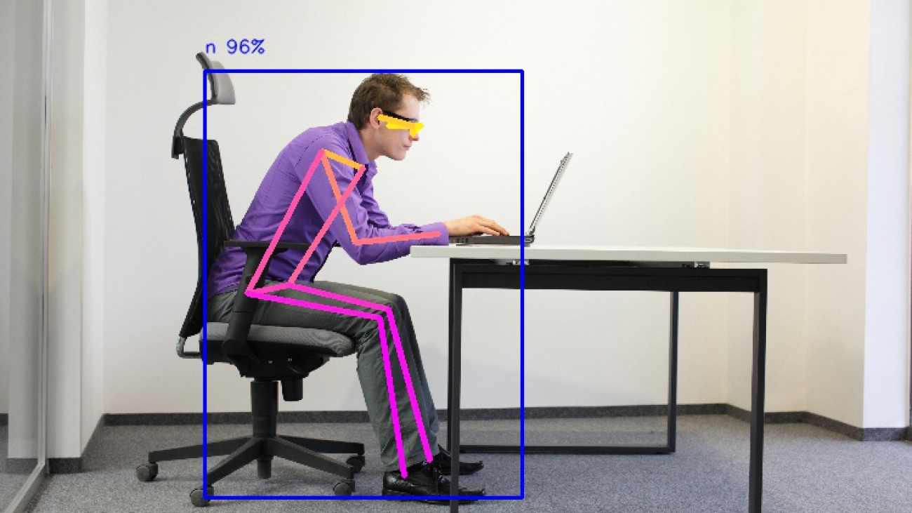
See use case section for how to build a posture tracker project with AWS DeepLens

Launches

As models become more sophisticated, AWS customers are increasingly applying machine learning (ML) prediction to video content, whether that’s in media and entertainment, autonomous driving, or more. At AWS, we had the following exciting July launches:

• On July 9, we announced that SageMaker Ground Truth now supports video labeling. The National Football League (NFL) has already put this new feature to work to develop labels for training a computer vision system that tracks all 22 players as they move on the field during plays. Amazon SageMaker Ground Truth reduced the timeline for developing a high-quality labeling dataset by more than 80%.
• On July 13, we launched the availability of AWS DeepRacer Evo and Sensor Kit for purchase. AWS DeepRacer Evo is available for a limited-time, discounted price of $399, a savings of $199 off the regular bundle price of $598, and the AWS DeepRacer Sensor Kit is available for $149, a savings of $100 off the regular price of $249. AWS DeepRacer is a fully autonomous 1/18th scale race car powered by reinforcement learning (RL) that gives ML developers of all skill levels the opportunity to learn and build their ML skills in a fun and competitive way. AWS DeepRacer Evo includes new features and capabilities to help you learn more about ML through the addition of sensors that enable object avoidance and head-to-head racing. Both items are available on com for shipping in the US only.
• On July 23, we announced that Contact Lens for Amazon Connect is now generally available. Contact Lens is a set of capabilities for Amazon Connect enabled by ML that gives contact centers the ability to understand the sentiment, trends, and compliance of customer conversations to improve their experience and identify crucial feedback.
• As of July 28, Amazon Fraud Detector is now generally available. Amazon Fraud Detector is a fully managed service that makes it easy to identify potentially fraudulent online activities such as online payment fraud and the creation of fake accounts. It uses your data, ML, and more than 20 years of fraud detection expertise from Amazon to automatically identify potentially fraudulent online activity so you can catch more fraud faster.
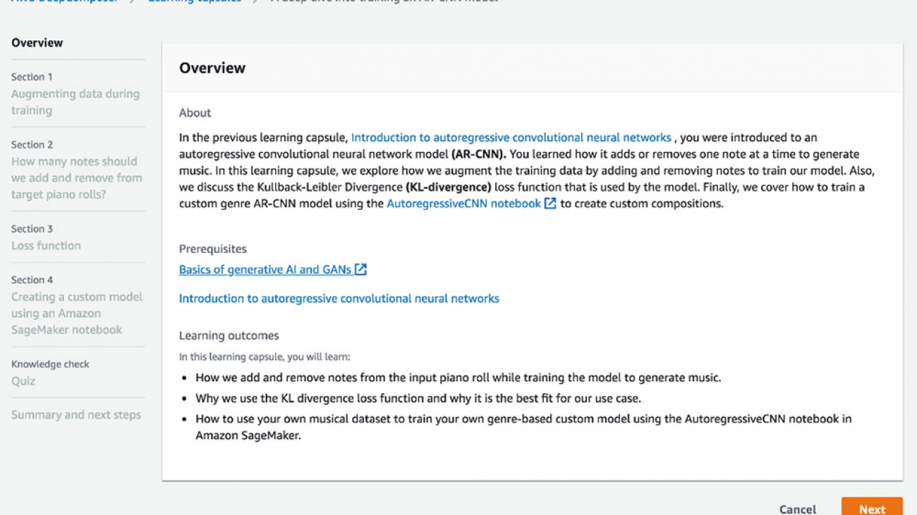
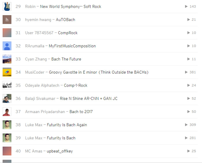
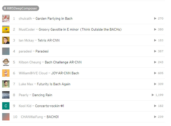
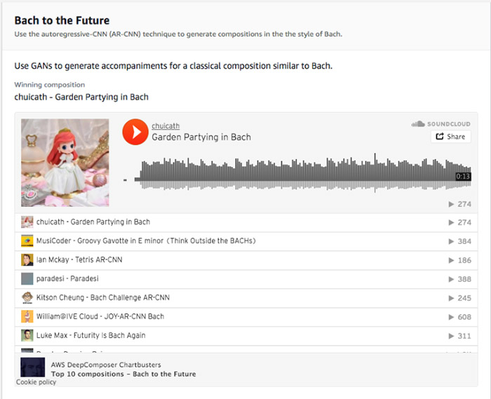
• Develop your own custom genre model to create AI-generated tunes in our latest AWS DeepComposer Chartbusters Challenge, Spin the Model. Submit your entries by 8/23 & see if you can top the #AI charts on SoundCloud for a chance to win some great prizes.

Use cases

Get ideas and architectures from AWS customers, partners, ML Heroes, and AWS experts on how to apply ML to your use case:

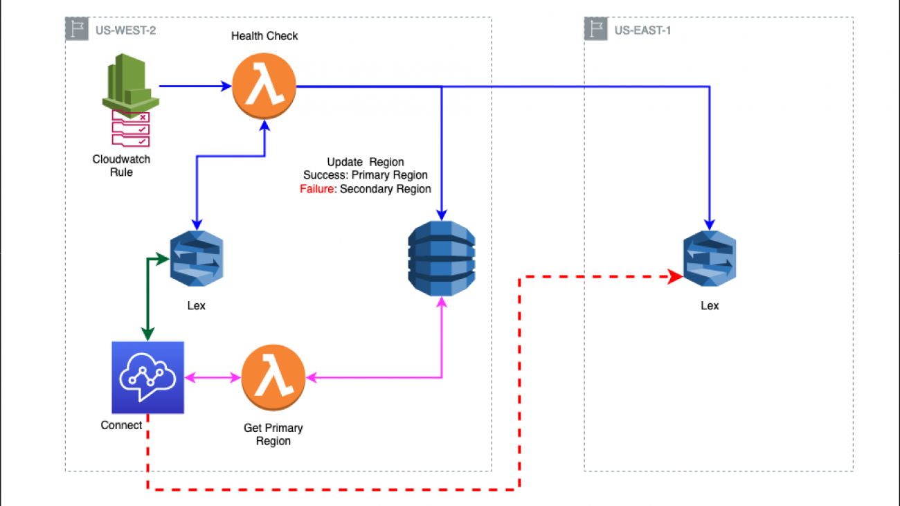
• AWS Machine Learning Hero Cyrus Wong shares how he developed Callouts, a simple, consistent, and scalable solution for educators to communicate with students using Amazon Connect and Amazon Lex. Learn how you can build your own scalable outbound call engine.
• The products Atlassian builds have hundreds of developers working on them, composed of a mixture of monolithic applications and microservices. When an incident occurs, it can be hard to diagnose the root cause due to the high rate of change within the code bases. Learn how implementing Amazon CodeGuru Profiler has enabled Atlassian developers to own and take action on performance engineering.
• Given the shift in customer trends to audio consumption, Amazon Polly launched a new speaking style focusing on the publishing industry: the Newscaster speaking style. Learn how the Newscaster voice was built and how you can use the Newscaster voice with your content in a few simple steps.
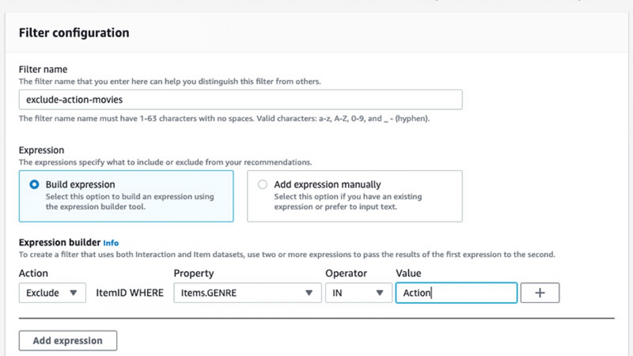
• Personalized recommendations can help improve customer engagement and conversion. Learn how Pulselive, a digital media sports technology company, increased video consumption by 20% with Amazon Personalize.
• Working from home can be a big change to your ergonomic setup, which can make it hard for you to keep a healthy posture and take frequent breaks throughout the day. To help you maintain good posture and have fun with ML in the process, you can build a posture tracker project with AWS DeepLens, the AWS programmable video camera for developers to learn ML.

Explore more ML stories

Want more news about developments in ML? Check out the following stories:

• Formula 1 Pit Strategy Battle – Take a deep dive into how the Amazon ML Solutions Lab and Professional Services Teams worked with Formula 1 to build a real-time race strategy prediction application using AWS technology that brings pit wall decisions to the viewer, and resulted in the Pit Strategy Battle graphic. You can also learn how a serverless architecture can provide ML predictions with minimal latency across the globe, and how to get started on your own ML journey.
• Fairness in AI – At the seventh Workshop on Automated Machine Learning (AutoML) at the International Conference on Machine Learning, Amazon researchers won a best paper award for the paper “Fair Bayesian Optimization.” The paper addresses the problem of ensuring the fairness of AI systems, a topic that has drawn increasing attention in recent years. Learn more about the research findings at Amazon.Science.

Mark your calendars

Join us for the following exciting ML events:

• Have fun while learning how to build, train, and deploy ML models with Amazon SageMaker Fridays. Join our expert ML Specialists Emily Webber and Alex McClure for a live session on Twitch. Register now!
• AWS Power Hour: Machine Learning is a weekly, live-streamed program that premiered Thursday, July 23, at 7:00 p.m. EST and will air at that time every Thursday for 7 weeks.

Also, if you missed it, see the Amazon Augmented AI (Amazon A2I) Tech Talk to learn how you can implement human reviews to review your ML predictions from Amazon Textract, Amazon Rekognition, Amazon Comprehend, Amazon SageMaker, and other AWS AI/ ML services.

See you next month for more on AWS ML!

About the author

Laura Jones is a product marketing lead for AWS AI/ML where she focuses on sharing the stories of AWS’s customers and educating organizations on the impact of machine learning. As a Florida native living and surviving in rainy Seattle, she enjoys coffee, attempting to ski and enjoying the great outdoors.

Read More

We’re pleased to announce enhancements to recommendation filters in Amazon Personalize, which provide you greater control on recommendations your users receive by allowing you to exclude or include items to recommend based on criteria that you define. For example, when recommending products for your e-retail store, you can exclude unavailable items from recommendations. If you’re recommending videos to users, you can choose to only recommend premium content if the user is in a particular subscription tier. You typically address this by writing custom code to implement their business rules, but you can now save time and streamline your architectures by using recommendation filters in Amazon Personalize.

Based on over 20 years of personalization experience, Amazon Personalize enables you to improve customer engagement by powering personalized product and content recommendations and targeted marketing promotions. Amazon Personalize uses machine learning (ML) to create high-quality recommendations for your websites and applications. You can get started without any prior ML experience using simple APIs to easily build sophisticated personalization capabilities in just a few clicks. Amazon Personalize processes and examines your data, identifies what is meaningful, automatically picks the right ML algorithm, and trains and optimizes a custom model based on your data. All of your data is encrypted to be private and secure, and is only used to create recommendations for your users.

Setting up and using recommendation filters is simple, taking only a few minutes to define and deploy your custom business rules with a real-time campaign. You can use the Amazon Personalize console or API to create a filter with your business logic using the Amazon Personalize domain specific language (DSL). You can apply this filter while querying for real-time recommendations using the GetRecommendations or GetPersonalizedRanking API, or while generating recommendations in batch mode through a batch inference job.

This post walks you through setting up and using item and user metadata-based recommendation filters in Amazon Personalize.

Prerequisites

To define and apply filters, you first need to set up the following Amazon Personalize resources. For instructions on the Amazon Personalize console, see Getting Started (Console).

1. Create a dataset group.
2. Create an Interactions dataset using the following schema and import data using the interactions-100k.csv data file:

   {
   	"type": "record",
   	"name": "Interactions",
   	"namespace": "com.amazonaws.personalize.schema",
   	"fields": [
   		{
   			"name": "USER_ID",
   			"type": "string"
   		},
   		{
   			"name": "ITEM_ID",
   			"type": "string"
   		},
   		{
   			"name": "EVENT_VALUE",
   			"type": [
   				"null",
   				"float"
   			]
   		},
   		{
   			"name": "TIMESTAMP",
   			"type": "long"
   		},
   		{
   			"name": "EVENT_TYPE",
   			"type": "string"
   		}
   	],
   	"version": "1.0"
   }
   

3. Create an Items dataset using the following schema and import data using the csv data file:

   {
   	"type": "record",
   	"name": "Items",
   	"namespace": "com.amazonaws.personalize.schema",
   	"fields": [
   		{
   			"name": "ITEM_ID",
   			"type": "string"
   		},
   		{
   			"name": "GENRE",
   			"type": "string"
   			"categorical": true
   		}
   	],
   	"version": "1.0"
   }
   

4. Create a solution using any recipe. In this post, we use the aws-hrnn recipe.
5. Create a campaign.

Creating your filter

Now that you have set up your Amazon Personalize resources, you can define and test custom filters.

Filter expression language

Amazon Personalize uses its own DSL called filter expressions to determine which items to exclude or include in a set of recommendations. Filter expressions are scoped to a dataset group. You can only use them to filter results for solution versions (an Amazon Personalize model trained using your datasets in the dataset group) or campaigns (a deployed solution version for real-time recommendations). Amazon Personalize can filter items based on user-item interaction, item metadata, or user metadata datasets.

The following are some examples of filter expressions by item:

• To remove all items in the "Comedy" genre, use the following filter expression:

  EXCLUDE ItemId WHERE item.genre in ("Comedy")

• To include items with a "number of downloads" less than 20, use the following filter expression:

  INCLUDE ItemId WHERE item.number_of_downloads < 20

The following are some examples of filter expressions by interaction:

• To remove items that have been clicked or streamed by a user, use the following filter expression:

  EXCLUDE ItemId WHERE interaction.event_type in ("click", "stream")

• To include items that a user has interacted with in any way, use the following filter expression:

  INCLUDE ItemId WHERE interactions.event_type in ("*")

You can also filter by user:

• To exclude items where the number of downloads is less than 20 if the current user’s age is over 18 but less than 30, use the following filter expression:

  EXCLUDE ItemId WHERE item.number_of_downloads < 20 IF CurrentUser.age > 18 AND CurrentUser.age < 30

You can also chain multiple expressions together, allowing you to pass the result of one expression to another in the same filter using a pipe ( | ) to separate them:

• The following filter expression example includes two expressions. The first expression includes items in the "Comedy" genre, and the result of this filter is passed to another expression that excludes items with the description "classic":

  INCLUDE Item.ID WHERE item.genre IN (“Comedy”) | EXCLUDE ItemID WHERE item.description IN ("classic”)

For more information, see Datasets and Schemas. For more information about filter definition DSL, see Filtering Recommendations.

Creating a filter on the console

You can use the preceding DSL to create a custom filter on the Amazon Personalize console. To create a filter, complete the following steps:

1. On the Amazon Personalize console, choose Filters.
2. Choose Create filter.
3. For Filter name, enter the name for your filter.
4. For Expression, select Build expression.

Alternatively, you can add your expression manually.

5. To chain additional expressions with your filter, choose +.
6. To add additional filter expressions, choose Add expression.
7. Choose Finish.

Creating a filter takes you to a page containing detailed information about your filter. You can view more information about your filter, including the filter ARN and the corresponding filter expression you created. You can also delete filters on this page or create more filters from the summary page.

You can also create filters via the createFilter API in Amazon Personalize. For more information, see Filtering Recommendations.

Applying your filter to real-time recommendations on the console

The Amazon Personalize console allows you to spot-check real-time recommendations on the Campaigns page. From this page, you can test your filters while retrieving recommendations for a specific user on demand. To do so, navigate to the Campaigns tab; this should be in the same dataset group that you used to create the filter. You can then test the impact of applying the filter on the recommendations.

Recommendations without a filter

The following screenshot shows recommendations returned with no filter applied.

Recommendations with a filter

The following screenshot shows results after you remove the "Action" genre from the recommendations by applying the filter we previously defined.

If we investigate the Items dataset provided in this example, item 546 is in the genre "Action" and we excluded the "Action" genre in our filter.

This information tells us that Item 546 should be excluded from recommendations. The results show that the filter removed items in the genre "Action" from the recommendation.

Applying your filter to batch recommendations on the console

To apply a filter to batch recommendations on the console, follow the same process as real-time recommendations. On the Create batch inference job page, choose the filter name to apply a previously created filter to your batch recommendations.

Applying your filter to real-time recommendations through the SDK

You can also apply filters to recommendations that are served through your SDK or APIs by supplying the filterArn as an additional and optional parameter to your GetRecommendations calls. Use "filterArn" as the parameter key and supply the filterArn as a string for the value. filterArn is a unique identifying key that the CreateFilter API call returns. You can also find a filter’s ARN on the filter’s detailed information page.

The following example code is a request body for the GetRecommendations API that applies a filter to a recommendation:

{
    "campaignArn": "arn:aws:personalize:us-west-2:000000000000:campaign/test-campaign",
    "userId": "1",
    "itemId": "1",
    "numResults": 5,
    "filterArn": "arn:aws:personalize:us-west-2:000000000000:filter/test-filter"
}

Applying your filter to batch recommendations through the SDK

To apply filters to batch recommendations when using a SDK, you provide the filterArn in the request body as an optional parameter. Use "filterArn" as the key and the filterArn as the value.

Summary

Customizable recommendation filters in Amazon Personalize allow you to fine-tune recommendations to provide more tailored experiences that improve customer engagement and conversion according to your business needs without having to implement post-processing logic on your own. For more information about optimizing your user experience with Amazon Personalize, see What Is Amazon Personalize?

About the Author

Matt Chwastek is a Senior Product Manager for Amazon Personalize. He focuses on delivering products that make it easier to build and use machine learning solutions. In his spare time, he enjoys reading and photography.

Read More

One of AWS’s goals is to put machine learning (ML) in the hands of every developer. With the open-source AutoML library AutoGluon, deployed using Amazon SageMaker and AWS Lambda, we can take this a step further, putting ML in the hands of anyone who wants to make predictions based on data—no prior programming or data science expertise required.

AutoGluon automates ML for real-world applications involving image, text, and tabular datasets. AutoGluon trains multiple ML models to predict a particular feature value (the target value) based on the values of other features for a given observation. During training, the models learn by comparing their predicted target values to the actual target values available in the training data, using appropriate algorithms to improve their predictions accordingly. When training is complete, the resulting models can predict the target feature values for observations they have never seen before, even if you don’t know their actual target values.

AutoGluon automatically applies a variety of techniques to train models on data with a single high-level API call—you don’t need to build models manually. Based on a user-configurable evaluation metric, AutoGluon automatically selects the highest-performing combination, or ensemble, of models. For more information about how AutoGluon works, see Machine learning with AutoGluon, an open source AutoML library.

To get started with AutoGluon, see the AutoGluon GitHub repo. For more information about trying out sophisticated AutoML solutions in your applications, see the AutoGluon website. Amazon SageMaker is a fully managed service that provides every developer and data scientist with the ability to build, train, and deploy ML models efficiently. AWS Lambda lets you run code without provisioning or managing servers, can be triggered automatically by other AWS services like Amazon Simple Storage Service (Amazon S3), and allows you to build a variety of real-time data processing systems.

With AutoGluon, you can achieve state-of-the-art predictive performance on new observations with as few as three lines of Python code. In this post, we achieve the same results with zero lines of code—making AutoML accessible to non-developers—by using AWS services to deploy a pipeline that trains ML models and makes predictions on tabular data using AutoGluon. After deploying the pipeline in your AWS account, all you need to do to get state-of-the-art predictions on your data is upload it to an S3 bucket with a provided AutoGluon package.

The code-free ML pipeline

The pipeline starts with an S3 bucket, which is where you upload the training data that AutoGluon uses to build your models, the testing data you want to make predictions on, and a pre-made package containing a script that sets up AutoGluon. After you upload the data to Amazon S3, a Lambda function kicks off an Amazon SageMaker model training job that runs the pre-made AutoGluon script on the training data. When the training job is finished, AutoGluon’s best-performing model makes predictions on the testing data, and these predictions are saved back to the same S3 bucket. The following diagram illustrates this architecture.

Deploying the pipeline with AWS CloudFormation

You can deploy this pipeline automatically in an AWS account using a pre-made AWS CloudFormation template. To get started, complete the following steps:

1. Choose the AWS Region in which you’d like to deploy the template. If you’d like to deploy it in another region, please download the template from GitHub and upload it to CloudFormation yourself.
   
   

   Northern Virginia
   Oregon
   Ireland
   Sydney

2. Sign in to the AWS Management Console.
3. For Stack name, enter a name for your stack (for example, code-free-automl-stack).
4. For BucketName, enter a unique name for your S3 bucket (for example, code-free-automl-yournamehere).
5. For TrainingInstanceType, enter your compute instance.

This parameter controls the instance type Amazon SageMaker model training jobs use to run AutoGluon on your data. AutoGluon is optimized for the m5 instance type, and 50 hours of Amazon SageMaker training time with the m5.xlarge instance type are included as part of the AWS Free Tier. We recommend starting there and adjusting the instance type up or down based on how long your initial job takes and how quickly you need the results.

6. Select the IAM creation acknowledgement checkbox and choose Create stack.
   
7. Continue with the AWS CloudFormation wizard until you arrive at the Stacks page.
   
   

It takes a moment for AWS CloudFormation to create all the pipeline’s resources. When you see the CREATE_COMPLETE status (you may need to refresh the page), the pipeline is ready for use.

9. To see all the components shown in the architecture, choose the Resources tab.
   
10. To navigate to the S3 bucket, choose the corresponding link.
    

Before you can use the pipeline, you have to upload the pre-made AutoGluon package to your new S3 bucket.

11. Create a folder called source in that bucket.
    
12. Upload the sourcedir.tar.gz package there; keep the default object settings.
    

Your pipeline is now ready for use!

Preparing the training data

To prepare your training data, go back to the root of the bucket (where you see the source folder) and make a new directory called data; this is where you upload your data.

Gather the data you want your models to learn from (the training data). The pipeline is designed to make predictions for tabular data, the most common form of data in real-world applications. Think of it like a spreadsheet; each column represents the measurement of some variable (feature value), and each row represents an individual data point (observation).

For each observation, your training dataset must include columns for explanatory features and the target column containing the feature value you want your models to predict.

Store the training data in a CSV file called <Name>_train.csv, where <Name> can be replaced with anything.

Make sure that the header name of the desired target column (the value of the very first row of the column) is set to target so AutoGluon recognizes it. See the following screenshot of an example dataset.

Preparing the test data

You also need to provide the testing data you want to make predictions for. If this dataset already contains values for the target column, you can compare these actual values to your model’s predictions to evaluate the quality of the model.

Store the testing dataset in another CSV file called <Name>_test.csv, replacing <Name> with the same string you chose for the corresponding training data.

Make sure that the column names match those of <Name>_train.csv, including naming the target column target (if present).

Upload the <Name>_train.csv and <Name>_test.csv files to the data folder you made earlier in your S3 bucket.

The code-free ML pipeline kicks off automatically when the upload is finished.

Training the model

When the training and testing dataset files are uploaded to Amazon S3, AWS logs the occurrence of an event and automatically triggers the Lambda function. This function launches the Amazon SageMaker training job that uses AutoGluon to train an ensemble of ML models. You can view the job’s status on the Amazon SageMaker console, in the Training jobs section (see the following screenshot).

Performing inference

When the training job is complete, the best-performing model or weighted combination of models (as determined by AutoGluon) is used to compute predictions for the target feature value of each observation in the testing dataset. These predictions are automatically stored in a new directory within a results directory in your S3 bucket, with the filename <Name>_test_predictions.csv.

AutoGluon produces other useful output files, such as <Name>_leaderboard.csv (a ranking of each individual model trained by AutoGluon and its predictive performance) and <Name>_model_performance.txt (an extended list of metrics corresponding to the best-performing model). All these files are available for download to your local machine from the Amazon S3 console (see the following screenshot).

Extensions

The trained model artifact from AutoGluon’s best-performing model is also saved in the output folder (see the following screenshot).

You can extend this solution by deploying that trained model as an Amazon SageMaker inference endpoint to make predictions on new data in real time or by running an Amazon SageMaker batch transform job to make predictions on additional testing data files. For more information, see Work with Existing Model Data and Training Jobs.

You can also reuse this automated pipeline with custom model code by replacing the AutoGluon sourcedir.tar.gz package we prepared for you in the source folder. If you unzip that package and look at the Python script inside, you can see that it simply runs AutoGluon on your data. You can adjust some of the parameters defined there to better match your use case. That script and all the other resources used to set up this pipeline are freely available in this GitHub repository.

Cleaning up

The pipeline doesn’t cost you anything more to leave up in your account because it only uses fully managed compute resources on demand. However, if you want to clean it up, simply delete all the files in your S3 bucket and delete the launched CloudFormation stack. Make sure to delete the files first; AWS CloudFormation doesn’t automatically delete an S3 bucket with files inside.

To delete the files from your S3 bucket, on the Amazon S3 console, select the files and choose Delete from the Actions drop-down menu.

To delete the CloudFormation stack, on the AWS CloudFormation console, choose the stack and choose Delete.

In the confirmation window, choose Delete stack.

Conclusion

In this post, we demonstrated how to train ML models and make predictions without writing a single line of code—thanks to AutoGluon, Amazon SageMaker, and AWS Lambda. You can use this code-free pipeline to leverage the power of ML without any prior programming or data science expertise.

If you’re interested in getting more guidance on how you can best use ML in your organization’s products and processes, you can work with the Amazon ML Solutions Lab. The Amazon ML Solutions Lab pairs your team with Amazon ML experts to prepare data, build and train models, and put models into production. It combines hands-on educational workshops with brainstorming sessions and advisory professional services to help you work backward from business challenges, and go step-by-step through the process of developing ML-based solutions. At the end of the program, you can take what you have learned through the process and use it elsewhere in your organization to apply ML to business opportunities.

About the Authors

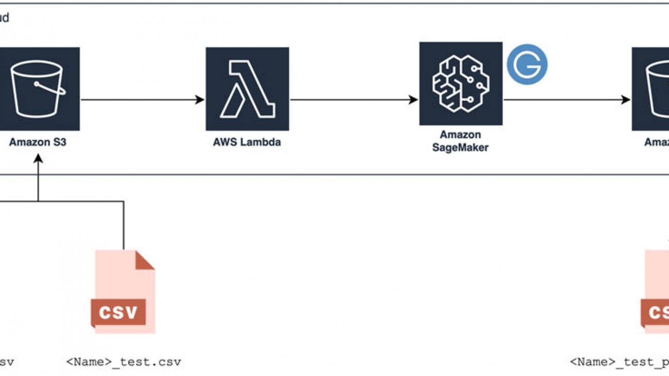
Abhi Sharma is a deep learning architect on the Amazon ML Solutions Lab team, where he helps AWS customers in a variety of industries leverage machine learning to solve business problems. He is an avid reader, frequent traveler, and driving enthusiast.

Ryan Brand is a Data Scientist in the Amazon Machine Learning Solutions Lab. He has specific experience in applying machine learning to problems in healthcare and the life sciences, and in his free time he enjoys reading history and science fiction.

Tatsuya Arai Ph.D. is a biomedical engineer turned deep learning data scientist on the Amazon Machine Learning Solutions Lab team. He believes in the true democratization of AI and that the power of AI shouldn’t be exclusive to computer scientists or mathematicians.

Read More

Whether your jam is reggae, hip-hop or electronic you can get creative and enter the latest AWS DeepComposer Chartbusters challenge! The Spin the Model challenge launches today and is open until August 23, 2020. AWS DeepComposer gives developers a creative way to get started with machine learning. Chartbusters is a monthly challenge where you can use AWS DeepComposer to create original compositions and compete to top the charts and win prizes.

To participate in the challenge you first need to train a model and create a composition using your dataset and the Amazon SageMaker notebook. You don’t need a physical keyboard to participate in the challenge. Next, you import the composition on the AWS DeepComposer console, and submit the composition to SoundCloud.  When you submit a composition, AWS DeepComposer automatically adds it to the Spin the Model challenge playlist in SoundCloud.

You can use the A deep dive into training an AR-CNN model learning capsule available on the AWS DeepComposer console to learn the concepts to train a model. To access the learning capsule, sign in to the AWS DeepComposer console and choose learning capsules in the navigation pane. Choose A deep dive into training an AR-CNN model to begin learning.

Training a model

We have provided a sample notebook to create a custom model. To use the notebook, first create the Amazon SageMaker notebook instance.

1. On the Amazon SageMaker console, under Notebook, choose Notebook instances.
   
2. Choose Create notebook instance.
   
3. For Notebook instance type, choose ml.c5.4xlarge.
   
4. For IAM role, choose a new or existing role.
5. For Root access, select Enable.
6. For Encryption key, choose No Custom Encryption.
   
7. For Repository, choose Clone a public Git repository to this notebook instance only.
8. For Git repository URL, enter https://github.com/aws-samples/aws-deepcomposer-samples.
9. Choose Create notebook instance.
10. Select your notebook instance and choose Open Jupyter.
    
11. In the ar-cnn folder, choose AutoRegressiveCNN.ipynb.

You’re likely prompted to choose a kernel.

11. From the drop-down menu, choose conda_tensorflow_p36.
12. Choose Set Kernel.

This notebook contains instructions and code to create and train a custom model from scratch.

13. To run the code cells, choose the code cell you want to run and choose Run.
    

If the kernel has an empty circle, it means it’s available and ready to run the code.

If the kernel has a filled circle, it means the kernel is busy. Wait for it to become available before you run the next line of code.

14. Provide the path for your dataset in the dataset summary section. Replace the current data_dir path with your dataset directory.

Your dataset should be in the .mid format.

15. After you provide the dataset directory path, you can experiment by changing the hyperparameters to train the model.

Training a model typically takes 5 hours or longer, depending on the dataset size and hyperparameter choices.

16. After you train the model, create a composition by using the code in the Inference section.

You can use the sample input MIDI files provided in the GitHub repo to generate a composition. Alternatively, you can play the input melody in AWS DeepComposer and download the melody to create a new composition.

17. After you create your composition, download it by navigating to the /outputs folder and choosing the file to download.

Submitting your composition

You can now import your composition in AWS DeepComposer. This step is necessary to submit the composition to the Spin the Model Chartbusters challenge.

1. On the AWS DeepComposer console, choose Input melody.
2. For Source of input melody, choose Imported track.
3. For Imported track, choose Choose file to upload the file.
4. Use the AR-CNN algorithm to further enhance the input melody.
   
5. To submit your composition for the challenge, choose Chartbusters in the navigation pane.
6. Choose Submit a composition.
7. Choose your composition from the drop-down menu.
8. Provide a track name for your composition and choose Submit.
   

AWS DeepComposer submits your composition to the Spin the Model playlist on SoundCloud. You can choose Vote on SoundCloud on the console to review and listen to other submissions for the challenge.

Conclusion

Congratulations! You have submitted your entry for the AWS DeepComposer Chartbusters challenge. Invite your friends and family to listen to and like your composition!

Learn more about AWS DeepComposer Chartbusters at https://aws.amazon.com/deepcomposer/chartbusters.

About the Author

Jyothi Nookula is a Principal Product Manager for AWS AI devices. She loves to build products that delight her customers. In her spare time, she loves to paint and host charity fund raisers for her art exhibitions.

Read More

We are excited to announce the top 10 compositions and the winner for the AWS DeepComposer Chartbusters Bach to the Future challenge. AWS DeepComposer gives developers a creative way to get started with machine learning. Chartbusters is a monthly challenge where you can use AWS DeepComposer to create original compositions and compete to top the charts and win prizes. The first challenge, Bach to the Future, required developers to use a new generative AI algorithm provided on the AWS DeepComposer console to create compositions in the style of Bach. It was an intense competition with high-quality submissions, making it a good challenge for our judges to select the chart-toppers!

Top 10 compositions

First, we shortlisted the top 20 compositions by using a total of customer likes and count of plays on SoundCloud. Then, our human experts (Mike Miller and Gillian Armstrong) and the AWS DeepComposer AI judge evaluated compositions for musical quality, creativity, and emotional resonance to select the top 10 ranked compositions.

The winner for the Bach to the Future challenge is… (cue drum roll) Catherine Chui! You can listen to the winning composition on SoundCloud. The top 10 compositions for the Bach to the Future challenge are:

You can listen to the playlist featuring the top 10 compositions on SoundCloud or on the AWS DeepComposer console.

The winner, Catherine Chui, will receive an AWS DeepComposer Chartbusters gold record. Catherine will be telling the story of how she created this tune and the experience of getting hands on with AWS DeepComposer in an upcoming post, right here on the AWS ML Blog.

Congratulations, Catherine Chui!

It’s time to move onto the next Chartbusters challenge — Spin the Model. The challenge launches today and is open until August 23, 2020. For more information about the competition and how to participate, see Announcing the AWS DeepComposer Chartbusters Spin the Model challenge.

About the Author

Jyothi Nookula is a Principal Product Manager for AWS AI devices. She loves to build products that delight her customers. In her spare time, she loves to paint and host charity fund raisers for her art exhibitions.

Read More

AWS customers rely on Amazon Lex bots to power their Amazon Connect self service conversational experiences on telephone and other channels. With Lex, callers (or customers, in Amazon Connect terminology) can get their questions conveniently answered regardless of agent availability. What architecture patterns can you use to make a bot resilient to service availability issues? In this post, we describe a cross-regional approach to yield higher availability by deploying Amazon Lex bots in multiple Regions.

Architecture overview

In this solution, Amazon Connect flows can achieve business continuity with minimal disruptions in the event of service availability issues with Amazon Lex. The architecture pattern uses the following components:

• Two Amazon Lex bots, each in a different Region.
• An Amazon Connect flow integrated with the bots triggered based on the result from the region check AWS Lambda function.
• A Lambda function to check the health of the bot.
• A Lambda function to read the Amazon DynamoDB table for the primary bot’s Region for a given Amazon Connect Region.
• A DynamoDB table to store a Region mapping between Amazon Connect and Amazon Lex. The health check function updates this table. The region check function reads this table for the most up-to-date primary Region mapping for Amazon Connect and Amazon Lex.

The goal of having identical Amazon Lex Bots in two Regions is to bring up the bot in the secondary Region and make it the primary in the event of an outage in the primary Region.

Multi-region pattern for Amazon Lex

The next two sections describe how an Amazon Connect flow integrated with an Amazon Lex bot can recover quickly in case of a service failure or outage in the primary Region and start servicing calls using Amazon Lex in the secondary Region.

The health check function calls one of the two Amazon Lex Runtime API calls—PutSession or PostText, depending on the TEST_METHOD Lambda environment variable. You can choose either one based on your preference and use case. The PutSession API call doesn’t have any extra costs associated with Amazon Lex, but it doesn’t test any natural language understanding (NLU) features of Amazon Lex. The PostTextAPI allows you to check the NLU functionality of Amazon Lex, but includes a minor cost.

The health check function updates the lexRegion column of the DynamoDB table (lexDR) with the Region name in which the test passed. If the health check passes the test in the primary Region, lexRegion gets updated with the name of the primary Region. If the health check fails, the function issues a call to the corresponding Runtime API based on the TEST_METHOD environment variable in the secondary Region. If the test succeeds, the lexRegion column in the DynamoDB table gets updated to the secondary Region; otherwise, it gets updated with err, which indicates both Regions have an outage.

On every call that Amazon Connect receives, it issues a region check function call to get the active Amazon Lex Region for that particular Amazon Connect Region. The primary Region returned by the region check function is the last entry written to the DynamoDB table by the health check function. Amazon Connect invokes the respective Get Customer Input Block configured with the Amazon Lex bot in the Region returned by the region check function. If the function returns the same Region as the Amazon Connect Region, it indicates that the health check has passed, and Amazon Connect calls the Amazon Lex bot in its same Region. If the function returns the secondary Region, Amazon Connect invokes the bot in the secondary Region.

Deploying Amazon Lex bots

You need to create an identical bot in both your primary and secondary Region. In this blog post, we selected us-east-1 as the primary and us-west-2 secondary Region. Begin by creating the bot in your primary Region, us-east-1.

1. On the Amazon Lex console, click Create.
2. In the Try a Sample section, select OrderFlowers.  Select COPPA to No
3. Leave all other settings at their default value and click Create.
4. The bot is created and will start to build automatically.
5. After your bot is built (in 1–2 minutes), choose Publish.
6. Create an alias with the name ver_one.

Repeat the above steps for us-west-2.  You should now have a working Amazon Lex bot in both us-east-1 and us-west-2.

Creating a DynamoDB table

Make sure your AWS Region is us-east-1.

1. On the DynamoDB console, choose Create.
2. For Table name, enter lexDR.
3. For Primary key, enter connectRegion with type String.
4. Leave everything else at their default and choose Create.
5. On the Items tab, choose Create item.
6. Set the connectRegion value to us-east-1 , and Append a new column of type String called lexRegion and set its value to us-east-1.
   
7. Click Save.
   

Creating IAM roles for Lambda functions

In this step, you create an AWS Identity and Access Management (IAM) for both Lambda functions to use.

1. On the IAM console, click on Access management and select Policies.
2. Click on Create Policy.
3. Click on JSON.
4. Paste the following custom IAM policy that allows read and write access to the DynamoDB table, lexDR. Replace the “xxxxxxxxxxxx” in the policy definition with your AWS Account Number.

   {
   	"Version": "2012-10-17",
   	"Statement": [{
   		"Sid": "VisualEditor0",
   		"Effect": "Allow",
   		"Action": ["dynamodb:GetItem", "dynamodb:UpdateItem"],
   		"Resource": "arn:aws:dynamodb:us-east-1:xxxxxxxxxxxx:table/lexDR"
   	}]
   }

5. Click on Review Policy.
6. Give it a name DynamoDBReadWrite and click on Create Policy.
7. On the IAM console, click on Roles  under Access management  and then click on Create Role.
8. Select Lambda for the service and click Next.
9. Attach the following permissions policies:
   1. AWSLambdaBasicExecutionRole
   2. AmazonLexRunBotsOnly
   3. DynamoDBReadWrite
10. Click Next: Tags. Skip the Tags page by clicking Next: Review.
11. Name the role lexDRRole. Click Save.

Deploying the region check function

You first create a Lambda function to read from the DynamoDB table to decide which Amazon Lex bot is in the same Region as the Amazon Connect instance. This function is later called by Amazon Connect or your application that’s using the bot.

1. On the Lambda console, choose Create function.
2. For Function name, enter lexDRGetRegion.
3. For Runtime, choose Python 3.8.
4. Under Permissions, choose Use an existing role.
5. Choose the role lexDRRole.
6. Choose Create function.
7. In the Lambda code editor, enter the following code (downloaded from lexDRGetRegion.zip):

   import json
   import boto3
   import os
   import logging
   dynamo_client=boto3.client('dynamodb')
   logger = logging.getLogger()
   logger.setLevel(logging.DEBUG)
    
   def getCurrentPrimaryRegion(key):
       result = dynamo_client.get_item(
           TableName=os.environ['TABLE_NAME'],
           Key = { 
               "connectRegion": {"S": key } 
           }
       )
       logger.debug(result['Item']['lexRegion']['S'] )
       return result['Item']['lexRegion']['S'] 
    
   def lambda_handler(event, context):
       logger.debug(event)
       region = event["Details"]["Parameters"]["region"]
       return {
           'statusCode': 200,
           'primaryCode': getCurrentPrimaryRegion(region)
       }

8. In the Environment variables section, choose Edit.
9. Add an environment variable with Key as TABLE_NAME and Value as lexDR.
10. Click Save to save the environment variable.
11. Click Save to save the Lambda function.

Deploying the health check function

Create another Lambda function in us-east-1 to implement the health check functionality.

1. On the Lambda console, choose Create function.
2. For Function name, enter lexDRTest.
3. For Runtime, choose Python 3.8.
4. Under Permissions, choose Use an existing role.
5. Choose lexDRRole.
6. Choose Create function.
7. In the Lambda code editor, enter the following code (downloaded from lexDRTest.zip):

   import json
   import boto3
   import sys
   import os
   
   dynamo_client = boto3.client('dynamodb')
   primaryRegion = os.environ['PRIMARY_REGION']
   secondaryRegion = os.environ['SECONDARY_REGION']
   tableName = os.environ['TABLE_NAME']
   primaryRegion_client = boto3.client('lex-runtime',region_name=primaryRegion)
   secondaryRegion_client = boto3.client('lex-runtime',region_name=secondaryRegion)
   
   def getCurrentPrimaryRegion():
       result = dynamo_client.get_item(
           TableName=tableName,
           Key={  
               'connectRegion': {'S': primaryRegion}  
           }
       )
       return result['Item']['lexRegion']['S'] 
       
   def updateTable(region):
       result = dynamo_client.update_item( 
           TableName= tableName,
           Key={  
               'connectRegion': {'S': primaryRegion } 
           },  
           UpdateExpression='set lexRegion = :region',
           ExpressionAttributeValues={
           ':region': {'S':region}
           }
       )
       
   #SEND MESSAGE/PUT SESSION ENV VA
   def put_session(botname, botalias, user, region):
       print(region,botname, botalias)
       client = primaryRegion_client
       if region == secondaryRegion:
           client = secondaryRegion_client
       try:
           response = client.put_session(botName=botname, botAlias=botalias, userId=user)
           if (response['ResponseMetadata'] and response['ResponseMetadata']['HTTPStatusCode'] and response['ResponseMetadata']['HTTPStatusCode'] != 200) or (not response['sessionId']):  
               return 501
           else:
               if getCurrentPrimaryRegion != region:
                   updateTable(region)
           return 200
       except:
           print('ERROR: {}',sys.exc_info()[0])
           return 501
   
   def send_message(botname, botalias, user, region):
       print(region,botname, botalias)
       client = primaryRegion_client
       if region == secondaryRegion:
           client = secondaryRegion_client
       try:
           message = os.environ['SAMPLE_UTTERANCE']
           expectedOutput = os.environ['EXPECTED_RESPONSE']
           response = client.post_text(botName=botname, botAlias=botalias, userId=user, inputText=message)
           if response['message']!=expectedOutput:
               print('ERROR: Expected_Response=Success, Response_Received='+response['message'])
               return 500
           else:
               if getCurrentPrimaryRegion != region:
                   updateTable(region)
               return 200
       except:
           print('ERROR: {}',sys.exc_info()[0])
           return 501
   
   def lambda_handler(event, context):
       print(event)
       botName = os.environ['BOTNAME']
       botAlias = os.environ['BOT_ALIAS']
       testUser = os.environ['TEST_USER']
       testMethod = os.environ['TEST_METHOD']
       if testMethod == 'send_message':
           primaryRegion_response = send_message(botName, botAlias, testUser, primaryRegion)
       else:
           primaryRegion_response = put_session(botName, botAlias, testUser, primaryRegion)
       if primaryRegion_response != 501:
           primaryRegion_client.delete_session(botName=botName, botAlias=botAlias, userId=testUser)
       if primaryRegion_response != 200:
           if testMethod == 'send_message':
               secondaryRegion_response = send_message(botName, botAlias, testUser, secondaryRegion)
           else:
               secondaryRegion_response = put_session(botName, botAlias, testUser, secondaryRegion)
           if secondaryRegion_response != 501:
               secondaryRegion_client.delete_session(botName=botName, botAlias=botAlias, userId=testUser)
           if secondaryRegion_response != 200:
               updateTable('err')
       #deleteSessions(botName, botAlias, testUser)
       return {'statusCode': 200,'body': 'Success'}
   

8. In the Environment variables section, choose Edit, and add the following environment variables:
   • BOTNAME – OrderFlowers
   • BOT_ALIAS – ver_one
   • SAMPLE_UTTERANCE – I would like to order some flowers.
     (The example utterance you want to use to send a message to the bot.)
   • EXPECTED_RESPONSE – What type of flowers would you like to order?
     (The expected response from the bot when it receives the above sample utterance.)
   • PRIMARY_REGION – us-east-1
   • SECONDARY_REGION – us-west-2
   • TABLE_NAME – lexDR
   • TEST_METHOD – put_session or send_message
     • send_message : This method calls the Lex Runtime function postText function which takes an utterance and maps it to one of the trained intents. postText will test the Natural Language Understanding capability of Lex. You will also iincur a small charge of $0.00075 per request)
     • put_session: This method calls the Lex Runtime function put_session function which creates a new session for the user. put_session will NOT test the Natual Language Understanding capability of Lex.)
   • TEST_USER – test
9. Click Save to save the environment variable.
10. In the Basic Settings section, update the Timeout value to 15 seconds.
11. Click Save to save the Lambda function.

Creating an Amazon CloudWatch rule

To trigger the health check function to run every 5 minutes, you create an Amazon CloudWatch rule.

1. On the CloudWatch console, under Events, choose Rules.
2. Choose Create rule.
3. Under Event Source, change the option to Schedule.
4. Set the Fixed rate of to 5 minutes
5. Under Targets, choose Add target.
6. Choose Lambda function as the target.
7. For Function, choose lexDRTest.
8. Under Configure input, choose Constant(JSON text), and enter {}
9. Choose Configure details.
10. Under Rule definition, for Name, enter lexHealthCheckRule.
11. Choose Create rule.

You should now have a lexHealthCheckRule CloudWatch rule scheduled to invoke your lexDRTest function every 5 minutes. This checks if your primary bot is healthy and updates the DynamoDB table accordingly.

Creating your Amazon Connect instance

You now create an Amazon Connect instance to test the multi-region pattern for the bots in the same Region where you created the lexDRTest function.

1. Create an Amazon Connect instance if you don’t already have one.
2. On the Amazon Connect console, choose the instance alias where you want the Amazon Connect flow to be.
3. Choose Contact flows.
4. Under Amazon Lex, select OrderFlowers bot from us-east-1 and click Add Lex Bot
5. Select OrderFlowers bot from us-west-2 and click Add Lex Bot
   
6. Under AWS Lambda, select lexDRGetRegion and click Add Lambda Function.
7. Log in to your Amazon Connect instance by clicking Overview in the left panel and clicking the login link.
8. Click Routing in the left panel, and then click Contact Flows in the drop down menu.
9. Click the Create Contact Flow button.
10. Click the down arrow button next to the Save button, and click on Import Flow.
11. Download the contact flow Flower DR Flow. Upload this file in the Import Flow dialog.
    
12. In the Contact Flow, Click on the Inovke AWS Lambda Function block, and it will open a properties panel on the right.
13. Select the lexDRGetRegion function and click Save.
14. Click on the Publish button to publish the contact flow.

Associating a phone number with the contact flow

Next, you will associate a phone number with your contact flow, so you can call in and test the OrderFlowers bot.

1. Click on the Routing option in the left navigation panel.
2. Click on Phone Numbers.
3. Click on Claim Number.
4. Select your country code and select a Phone Number.
5. In the Contact flow/IVR select box, select the contact flow Flower DR Flow imported in the earlier step.
6. Wait for a few minutes, and then call into that number to interact with the OrderFlowers bot.

Testing your integration

To test this solution, you can simulate a failure in the us-east-1 Region by implementing the following:

1. Open Amazon Lex Console in us-east-1 Region
2. Select the OrderFlowers bot.
3. Click on Settings.
4. Delete the bot alias ver_one

When the health check runs the next time, it will try to communicate with the Lex Bot in us-east-1 region. It will fail in getting a successful response, as the bot alias no longer exists. So, it will then make the call to the secondary Region, us-west-2. Upon receiving a successful response. Upon receiving this response, it will update the lexRegion column in the lexDR, DynamoDB table with us-west-2.

After this, all subsequent calls to Connect in us-east-1 will start interacting with the Lex Bot in us-west-2. This automatic switch over demonstrates how this architectural pattern can help achieve business continuity in the event of a service failure.
Between the time you delete the bot alias, and the next health check run, calls to Amazon Connect will receive a failure. However, after the health check runs, you will see a continuity in business operational automatically. The smaller the duration between your health check runs, the shorter the outage you will have. The duration between your health check runs can be changed by editing the Amazon CloudWatch rule, lexHealthCheckRule .

To make the health check pass in us-east-1 again, recreate the ver_one alias of the OrderFlowers bot in us-east-1.

Cleanup

To avoid incurring any charges in the future, delete all the resources created above.

1. Amazon Lex bot OrderFlowers created in us-east-1 and us-west-2
2. The Cloudwatch rule lexHealthCheckRule
3. The DynamoDB Table lexDR
4. The Lambda functions lexDRTest and lexDRGetRegion
5. Delete the IAM role lexDRRole
6. Delete the Contact Flow Flower DR Flow

Conclusion

Coupled with Amazon Lex for self-service, Amazon Connect allows you to easily create intuitive customer service experiences. This post offers a multi-region approach for high availability so that, if a bot or the supporting fulfillment APIs are under pressure in one Region, resources from a different Region can continue to serve customer demand.

About the Authors

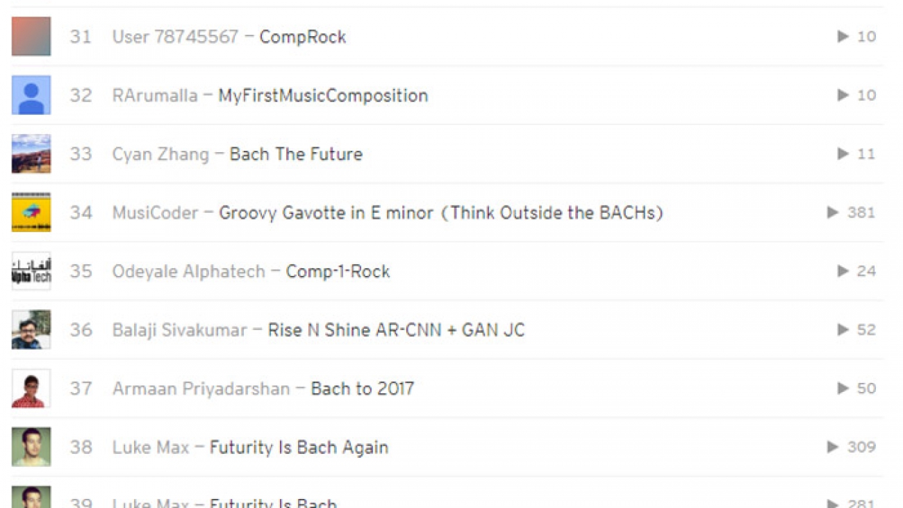
Shanthan Kesharaju is a Senior Architect in the AWS ProServe team. He helps our customers with their Conversational AI strategy, architecture, and development. Shanthan has an MBA in Marketing from Duke University, MS in Management Information Systems from Oklahoma State University, and a Bachelors in Technology from Kakaitya University in India. He is also currently pursuing his third Masters in Analytics from Georgia Tech.

Soyoung Yoon is a Conversation A.I. Architect at AWS Professional Services where she works with customers across multiple industries to develop specialized conversational assistants which have helped these customers provide their users faster and accurate information through natural language. Soyoung has M.S. and B.S. in Electrical and Computer Engineering from Carnegie Mellon University.

Read More