Monthly Archives: December 2020

Sharing data and computing in the cloud allows data users to focus on data analysis rather than data access. Open Data on AWS helps you discover and share public open datasets in the cloud. The Registry of Open Data on AWS hosts a large amount of public open data. The datasets range from genomics to climate to transportation information. They are well structured and easily accessible. Additionally, you can use these datasets in machine learning (ML) model development in the cloud.

In this post, we demonstrate how to extract buildings and roads from two large-scale geospatial datasets: SpaceNet satellite images and USGS 3DEP LiDAR data. Both datasets are hosted on the Registry of Open Data on AWS. We show you how to launch an Amazon SageMaker notebook instance and walk you through the tutorial notebooks at a high level. The notebooks reproduce winning algorithms from the SpaceNet challenges (which only use satellite images). In addition to the SpaceNet satellite images, we compare and combine the USGS 3D Elevation Program (3DEP) LiDAR data to extract the same.

This post demonstrates running ML services on AWS to extract features from large-scale geospatial data in the cloud. By following our examples, you can train the ML models on AWS, apply the models to other regions where satellite or LiDAR data is available, and experiment with new ideas to improve the performances. For the complete code and notebooks of this tutorial, see our GitHub repo.

Datasets

In this section, we provide more detail about the datasets we use in this post.

SpaceNet dataset

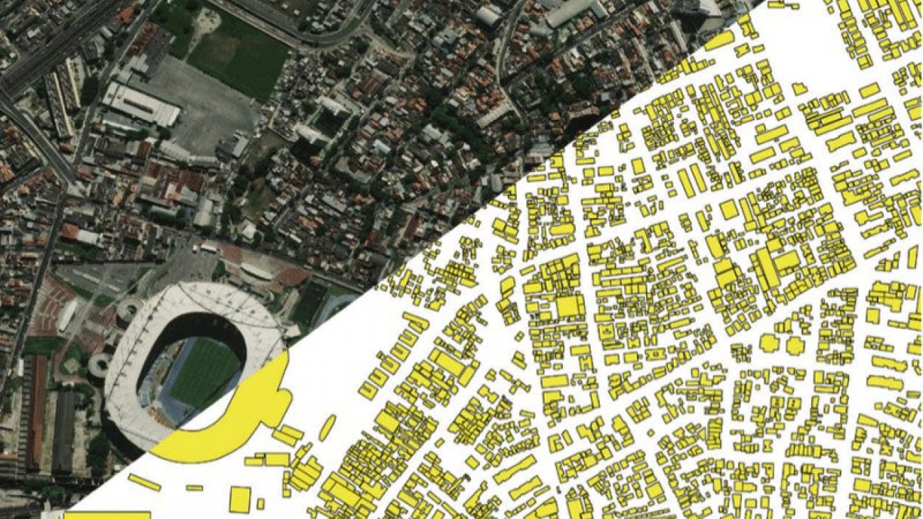
SpaceNet launched in August 2016 as an open innovation project offering a repository of freely available imagery with co-registered map features. It’s a large corpus of labeled satellite imagery. The project has also launched a series of competitions ranging from automatic building extraction, road extraction, to recently published multi-temporal urban development analysis. The dataset covers 11 areas of interest (AOIs), including Rio de Janeiro, Las Vegas, and Paris. For this post, we use Las Vegas; the images in this AOI cover 216km2 areas with 151,367 building polygon labels and 3,685km road labels.

The following image is from DigitalGlobe’s SpaceNet Challenge Concludes First Round, Moves to Higher Resolution Challenges.

USGS 3DEP LiDAR dataset

Our second dataset comes from the USGS 3D Elevation Program (3DEP) in the form of LiDAR (Light Detection and Ranging) data. The program’s goal is to complete the acquisition of nationwide LiDAR to provide the first-ever national baseline of consistent high-resolution topographic elevation data, collected in a timeframe of less than a decade. LiDAR is a remote sensing method that emits hundreds of thousands of near-infrared light pulses each second to measure distances to the Earth. These light pulses generate precise, 3D information about the shape of the Earth and its surface characteristics.

The USGS 3DEP LiDAR is presented in two formats. The first is a public repository in Entwine Point Tiles (EPT) format, which is a lossless, full resolution, streamable octree structure. This format is suitable for online visualization. The following image shows an example of LiDAR visualization in Las Vegas.

The other format is in LAZ (compressed LAS) with requester-pays access. In this post, we use LiDAR data in the second format.

Data registration

For this post, we select the Las Vegas AOI where both SpaceNet satellite images and USGS LiDAR data are available. Among SpaceNet data categories, we use the 30cm resolution pan-sharpened 3-band RGB geotiff and corresponding building and road labels. To improve the visual feature extraction performance, we process the data by white balancing and convert it to 8-bit (0–255) values for ease of postprocessing. The following graph shows the RGB value aggregated histogram of all images after processing.

Satellite images are 2D images, whereas the USGS LiDAR data are 3D point clouds and therefore require conversion and projection to align with 2D satellite images. We use Matlab and LAStools to map each 3D LiDAR point to a pixel-wise location corresponding to SpaceNet tiles, and generate two sets of attribute images: elevation and reflectivity intensity. The elevation ranges from approximately 2,000–3,000 feet, and the intensity ranges from 0–5,000 units. The following graphs show the aggregated histograms of all images for elevation and reflectivity intensity values.

Finally, we merge either one of the LiDAR attributes and merge them with the RGB images. The images are saved in 16-bit because LiDAR attribute values can be larger than 255, the 8-bit upper limit. We make this processed and merged data available via a publicly accessible Amazon Simple Storage Service (Amazon S3) bucket for this tutorial. The following are three samples of merged RGB+LiDAR images. From left to right, the columns are RGB image, LiDAR elevation attribute, and LiDAR reflectivity intensity attribute.

Creating a notebook instance

SageMaker is a fully managed service that allows you to build, train, deploy, and monitor ML models. Its modular design allows you to pick and choose features that suit your use cases at different stages of the ML lifecycle. SageMaker offers capabilities that abstract the heavy lifting of infrastructure management and provide the agility and scalability you desire for large-scale ML activities with different features and a pay-as-you-use pricing model.

The SageMaker on-demand notebook instance is a fully managed compute instance running the Jupyter Notebook app. SageMaker manages creating instances and related resources. Notebooks contain everything needed to run or recreate an ML workflow. You can use Jupyter notebooks in your notebook instance to prepare and process data, write code to train models, deploy models to SageMaker hosting, and test or validate your models. For different problems, you can select the type of instance to best fit each scenario (such as high throughput, high memory usage, or real-time inference).

Although training the deep learning model can take a long time, you can reproduce the inference part of this post with a reasonable computing cost. It’s recommended to run the notebooks inside a SageMaker notebook instance of type ml.p3.8xlarge (4 x V100 GPUs) or larger. Network training and inference is a memory-intensive process; if you run into out of memory or out of RAM errors, consider decreasing the batch_size in the configuration files (.yml format).

To create a notebook instance, complete the following steps:

1. On the SageMaker console, choose Notebook instances.
2. Choose Create notebook instance.
3. Enter the name of your notebook instance, such as open-data-tutorial.
4. Set the instance type to 8xlarge.
5. Choose Additional configuration.
6. Set the volume size to 60 GB.
7. Choose Create notebook instance.
8. When the instance is ready, choose Open in JupyterLab.
9. From the launcher, you can open a terminal and run the provided code.

Deploy environment and download datasets

At the JupyterLab terminal, run the following commands:

$ cd ~/SageMaker/$ ./setup-env.sh tutorial_env
$ git clone https://github.com/aws-samples/aws-open-data-satellite-lidar-tutorial.git
$ cd aws-open-data-satellite-lidar-tutorial

This downloads the tutorial repository from GitHub and takes you to the tutorial directory.

Next, set up a Conda environment by running setup-env.sh (see the following code). You can change the environment name from tutorial_env to any other name.

$ ./setup-env.sh tutorial_env

This may take 10–15 minutes to complete, after which you have a new Jupyter kernel called conda_tutorial_env, or conda_[name] if you change the environment name. You may need to wait a few minutes after conda completion and refresh the Jupyter page.

Next, download the necessary data from the public S3 bucket hosting the tutorial files:

$ ./download-from-s3.sh

This may take up to 5 minutes to complete and requires at least 23 GB of notebook instance storage.

Building extraction

Launch the notebook Building-Footprint.ipynb to reproduce this chapter.

The first and second SpaceNet challenges aimed to extract building footprints from satellite images at various AOIs. The fourth SpaceNet challenge posed a similar task with more challenging off-nadir ( oblique-looking angles) imagery. We reproduce a winning algorithm and evaluate its performance with both RGB images and LiDAR data.

Training data

In the Las Vegas AOI, SpaceNet data is tiled to size 200m x 200m. We select 3,084 tiles in which both SpaceNet imagery and LiDAR data are available and merge them together. Unfortunately, the labels of test data for scoring in the SpaceNet challenges are not published, so we split the merged data into 70% and 30% for training and evaluation. Between LiDAR elevation and intensity, we choose elevation for building extractions. See the following code:

In the Las Vegas AOI, SpaceNet data is tiled to size 200m×200m. We select 3084 tiles where both SpaceNet imagery and LiDAR data are available and merge them together. Unfortunately, the labels of test data for scoring in the SpaceNet challenges are not published, so we split the merged data by 70%/30% for training and evaluation. Between LiDAR elevation and intensity, we choose elevation for building extractions.

# Create Pandas data frame, containing columns 'image' and 'label'.
total_df = pd.DataFrame({'image': img_path_list
                         'label': mask_path_list})
# Split this data frame to training data and blind test data.
split_mask = np.random.rand(len(total_df)) < 0.7
train_df = total_df[split_mask]
test_df = total_df[~split_mask]

Model

We reproduce the winning algorithm from SpaceNet challenge 4 by XD_XD. The model has a U-net architecture with skip-connections between encoder and decoder, and a modified VGG16 as backbone encoder. The model takes three different types of input:

• Three-channel RGB image, same as the original contest
• One-channel LiDAR elevation image
• Four-channel RGB+LiDAR merged image

We train three models based on the three types of inputs described in this post and compare their performances.

The label for training is binary mask converted from polygon geojson by Solaris, an ML pipeline library developed by CosmiQ Works. We select a combined loss of binary cross-entropy and Jaccard loss with a weight factor alpha=0.8:

mathcal{L} =
alphamathcal{L}_mathrm{BCE} + (1 –
alphamathcal{L}_mathrm{Jaccard})

We train the models with batch size 20, Adam optimizer, and 10-4 learning rate for 100 epochs. The training takes approximately 100 minutes to finish on an ml.p3.8xlarge SageMaker notebook instance. See the following code:

# Load customized multi-channel input VGG16-Unet model.
from networks.vgg16_unet import get_modified_vgg16_unet

custom_model = get_modified_vgg16_unet(
    in_channels=config['data_specs']['channels'])
custom_model_dict = {
    'model_name': 'modified_vgg16_unet',
    'arch': custom_model}

# Select config file and link training datasets.
config = sol.utils.config.parse('./configs/buildings/RGB+ELEV.yml')
config['training_data_csv'] = train_csv_path
# Create solaris trainer, and train with configuration.
trainer = sol.nets.train.Trainer(config, custom_model_dict=custom_model_dict)
trainer.train()

The following images show examples of building extraction inputs and outputs. From left to right, the columns are RGB image, LiDAR elevation image, model prediction trained with RGB and LiDAR data, and ground truth building footprint mask.

Evaluation

Use the trained model to perform model inference on the test dataset (30% hold-out):

custom_model_dict = {
    'model_name': 'modified_vgg16_unet',
    'arch': custom_model,
    'weight_path': config['training']['model_dest_path']}
config['train'] = False

# Create solaris inferer, and do inference on test data.
inferer = sol.nets.infer.Inferer(config, custom_model_dict=custom_model_dict)
inferer(test_df)

After model inference, we evaluate the model performance using the same metric as in the original contest: an aggregated F-1 score with intersection of union (IoU) ≥ 0.5 criterion. There are two steps to compute this score. First, convert the building footprint binary masks to proposed polygons:

# Convert these probability maps to building polygons.
def pred_to_prop(pred_file, img_path):
    pred_path = os.path.join(pred_dir, pred_file)
    pred = skimage.io.imread(pred_path)[..., 0]
    prop_file = 
        pred_file.replace('RGB+ELEV', 'geojson_buildings').replace('tif', 'geojson')
    prop_path = os.path.join(prop_dir, prop_file)
    prop = sol.vector.mask.mask_to_poly_geojson(
        pred_arr=pred,
        reference_im=img_path,
        do_transform=True,
        min_area=1e-10,
        output_path=prop_path)

Next, compare the proposed polygons against the ground truth polygons (SpaceNet building labels), and count the aggregated F-1 scores:

# Evaluate aggregated F-1 scores.
def compute_score(prop_path, bldg_path):
    evaluator = sol.eval.base.Evaluator(bldg_path)
    evaluator.load_proposal(prop_path, conf_field_list=[])
    score = evaluator.eval_iou(miniou=0.5, calculate_class_scores=False)
    # score_list.append(score[0]) # skip because single-class
    return score[0] # single-class

The following table shows the F-1 scores from the three models trained with RGB images, LiDAR elevation images, and RGB+LiDAR merged images. Compared to using RGB only as in the original SpaceNet competition, the model trained using only LiDAR elevation images achieves a score only a few percent worse. When combining both RGB and LiDAR elevation in training, the model outperforms the RGB-only model. For reference, the F-1 scores of the top three teams from SpaceNet challenge 2 in this AOI are 0.885, 0.829, and 0.787 (we don’t compare them directly because they use a different test set for scoring).

Road extraction

To reproduce this section, launch the notebook Road-Network.ipynb.

The third SpaceNet challenge aimed to extract road networks from satellite images. The fifth SpaceNet challenge added predicting road speed along with the road network extraction in order to minimize travel time and plan optimal routing. Similar to building extraction, we reproduce a top winning algorithm, train different models with either RGB images, LiDAR attributes, or both of them, and evaluate their performance.

Training data

The road network extraction uses larger tiles with size 400m x 400m. We generate 918 merged tiles, and split by 70%/30% for training and evaluation. In this case, we select reflectivity intensity for road extraction because road surfaces often consist of materials that have distinctive reflectivity among backgrounds, such as a paved surface, dirt road, or asphalt.

Model

We reproduce the CRESI algorithm for road networks extraction. It also has a U-net architecture but uses ResNet as the backbone encoder. Again, we train the model with three different types of input:

• Three-channel RGB image
• One-channel LiDAR intensity image
• Four-channel RGB+LiDAR merged image

To extract road location and speed together, binary road mask doesn’t provide enough information for training. As mentioned in the CRESI paper, we can convert the speed metadata to either continuous mask (0–1 values) or multi-class binary mask. Because their test results show that multi-class binary mask performs better, we use the latter conversion scheme. The following images break down the eight-class road masks. The first seven binary masks represent road corresponds to seven bins of speed within 0–65 mph. The eighth mask (bottom right) represents the aggregation of all previous masks.

The following images show the visualization of multi-class road masks. The left is the RGB image tile. The right is the road mask with color coding in which the yellow-to-red colormap represents speed values from low to high speed (0–65 mph).

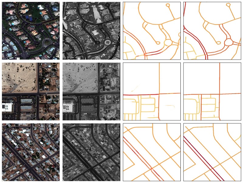
We train the model with the same setup as in the building extraction. The following images show examples of road extraction inputs and outputs. From left to right, the columns are RGB image, LiDAR reflectivity intensity image, model prediction trained with RGB and LiDAR data, and ground truth road mask.

Evaluation

We implement the average path length similarity (APLS) score to evaluate the road extraction performance. This metric is used in SpaceNet road challenges because APLS considers both logical topology (connections within road network) and physical topology (location of the road edges and nodes). The APLS can be weighted by either length or travel time; a higher score means better performance. See the following code:

# Skeletonize the prediction mask into non-geo road network graph.
!python ./libs/apls/skeletonize.py --results_dir={results_dir}
# Match geospatial info and create geo-projected graph.
!python ./libs/apls/wkt_to_G.py --imgs_dir={img_dir} --results_dir={results_dir}
# Infer road speed on each graph edge based on speed bins.
!python ./libs/apls/infer_speed.py --results_dir={results_dir} 
    --speed_conversion_csv_file='./data/roads/speed_conversion_binned7.csv'

# Compute length-based APLS score.
!python ./libs/apls/apls.py --output_dir={results_dir} 
    --truth_dir={os.path.join(data_dir, 'geojson_roads_speed')} 
    --im_dir={img_dir} 
    --prop_dir={os.path.join(results_dir, 'graph_speed_gpickle')} 
    --weight='length'

# Compute time-based APLS score.
!python ./libs/apls/apls.py --output_dir={results_dir} 
    --truth_dir={os.path.join(data_dir, 'geojson_roads_speed')} 
    --im_dir={img_dir} 
    --prop_dir={os.path.join(results_dir, 'graph_speed_gpickle')} 
    --weight='travel_time_s'

We convert multi-class road mask predictions to skeleton and speed-weighted graph and compute APLS scores. The following table shows the APLS scores of the three models. Similar to the building extraction results, the LiDAR-only result achieves scores close to the RGB-only result, whereas RGB+LiDAR gives the best performance.

Conclusion

We demonstrate how to extract building extract buildings and roads from two large-scale geospatial datasets hosted on the Registry of Open Data on AWS using a SageMaker notebook instance. The SageMaker notebook instance contains everything needed to run or recreate an ML workflow. It’s easy to use and customize to best fit different scenarios.

By using the LiDAR dataset from the Registry of Open Data on AWS and reproducing winning algorithms from SpaceNet building and road challenges, we show that you can use LiDAR data to perform the same task with similar accuracy, and even outperform the RGB models when combined.

With the full code and notebooks shared on GitHub and the necessary data hosted in the public S3 bucket, you can reproduce the map feature extraction tasks, apply the models to any other area of interest, and innovate with new ideas to improve model performance. For the complete code and notebooks of this tutorial, see our GitHub repo.

About the Authors

Yunzhi Shi is a data scientist at the Amazon ML Solutions Lab where he helps AWS customers address business problems with AI and cloud capabilities. Recently, he has been building computer vision, search, and forecast solutions for various customers.

Xin Chen is a senior manager at Amazon ML Solutions Lab, where he leads the Automotive Vertical and helps AWS customers across different industries identify and build machine learning solutions to address their organization’s highest return-on-investment machine learning opportunities. Xin obtained his Ph.D. in Computer Science and Engineering from the University of Notre Dame.

Tianyu Zhang is a data scientist at the Amazon ML Solutions Lab. He helps AWS customers solve business problems by applying ML and AI techniques. Most recently, he has built NLP model and predictive model for procurement and sports.

Read More

Earlier in 2020, widely used browsers like Chrome and Firefox changed their default behavior for rotating images based on image metadata, referred to as EXIF data. Previously, images always displayed in browsers exactly how they’re stored on disk, which is typically unrotated. After the change, images now rotate according to a piece of image metadata called orientation value. This has important implications for the entire machine learning (ML) community. For example, if the EXIF orientation isn’t considered, applications that you use to annotate images may display images in unexpected orientations and result in confusing or incorrect labels.

For example, before the change, by default images would display in the orientation stored on the device, as shown in the following image. After the change, by default, images display according to the orientation value in EXIF data, as shown in the second image.

Here, the image was stored in portrait mode, with EXIF data attached to indicate it should be displayed with a landscape orientation.

To ensure images are predictably oriented, ML annotation services need to be able to view image EXIF data. The recent change to global web standards requires you to grant explicit permission to image annotation services to view your image EXIF data.

To guarantee data consistency between workers and across datasets, the annotation tools used by Amazon SageMaker Ground Truth, Amazon Augmented AI (Amazon A2I), and Amazon Mechanical Turk need to understand and control orientations of input images that are shown to workers. Therefore, from January 12, 2021, onward, AWS requires that you add a cross-origin resource sharing (CORS) header configuration to Amazon Simple Storage Service (Amazon S3) buckets that contain labeling job or human review task input data. This policy allows these AWS services to view EXIF data and verify that images are predictably oriented in labeling and human review tasks.

This post provides details on the image metadata change, how it can impact labeling jobs and human review tasks, and how you can update your S3 buckets with these new, required permissions.

What is EXIF data?

EXIF data is metadata that tells us things about the image. EXIF data typically includes the height and width of an image but can also include things like the date a photo was taken, what kind of camera was used, and even GPS coordinates where the image was captured. For the image annotation web application community, the orientation property of EXIF is about to become very important.

When you take a photo, whether it’s landscape or portrait, the data is written to storage in the landscape orientation. Instead of storing a portrait photo in the portrait orientation, the camera writes a piece of metadata to the image to explain to applications how that image should be rotated when it’s shown to humans. To learn more, see Exif.

A big change to browsers: Why EXIF data is important

Until recently, popular web browsers such as Chrome and Firefox didn’t use EXIF orientation values, meaning that images that users annotated were never rotated. This means the annotation data matched how the image was stored and the orientation value didn’t matter.

Earlier in 2020, Chrome and Firefox changed their default behavior to begin using EXIF data by default. To make sure image annotating tasks weren’t impacted, AWS mitigated this change by preventing rotation so that users continued to annotate images in their unrotated form. However, AWS can no longer automatically prevent the rotation of images because the web standards group W3C has decided that the ability to control image rotation violates the web’s Same Origin Policy.

It is estimated that, starting with Chrome 88 on January 19^th, 2021, annotation services like the ones offered by AWS will require additional permissions to control the orientation of your images when displayed to human workers.

When using AWS services, you can grant these permissions by adding a CORS header policy to the S3 buckets that contain your input images.

Upcoming change to AWS image annotation job security requirements

It is recommended you add a CORS configuration to all S3 buckets that contain input data used for active and future labeling jobs as soon as possible. Starting January 12^th, 2021, to ensure human workers annotate your input images in a predictable orientation when you submit requests to create one of the following, you must add a CORS header policy to the S3 buckets that contain your input images:

• Ground Truth labeling jobs
• Amazon A2I human loops
• Mechanical Turk HITs

If you have pre-existing active resources like Ground Truth streaming labeling jobs, you must add a CORS header policy to the S3 bucket used to create those resources. For Ground Truth, this is the input data S3 bucket identified when you created the streaming labeling job.

Additionally, if you reuse resources, such as cloning a Ground Truth labeling job, make sure the input data S3 bucket you use has a CORs header policy attached.

In the context of input image data, AWS services use CORS headers to view EXIF orientation data to control image rotation.

If you don’t add a CORS header policy to an S3 bucket that contains input data by January 12^th, 2021, Ground Truth, Amazon A2I, and Mechanical Turk tasks created using this S3 bucket will fail.

Adding a CORS header policy to an S3 bucket

If you’re creating an Amazon A2I human loop or Mechanical Turk job, or you’re using the CreateLabelingJob API to create a Ground Truth labeling job, you can add a CORS policy to an S3 bucket that contains input data on the Amazon S3 console.

If you create your job through the Ground Truth console, under Enable enhanced image access, a check box is select to enable CORS configuration on the S3 bucket that contains your input manifest file as shown in the following image. Keep this check box selected. If all of your input data is not located in the same S3 bucket as your input manifest file, you must manually add a CORS configuration to all S3 buckets that contain input data using the following instructions.

For instructions on setting the required CORS headers on the S3 bucket that hosts your images, see How do I add cross-domain resource sharing with CORS? Use the following CORS configuration code for the buckets that host your images.

The following is the code in JSON format:

[{
   "AllowedHeaders": [],
   "AllowedMethods": ["GET"],
   "AllowedOrigins": ["*"],
   "ExposeHeaders": []
}]

The following is the code in XML format:

<CORSConfiguration>
 <CORSRule>
   <AllowedOrigin>*</AllowedOrigin>
   <AllowedMethod>GET</AllowedMethod>
 </CORSRule>
</CORSConfiguration>

The following GIF demonstrates the instructions found in the Amazon S3 documentation to add a CORS header policy using the Amazon S3 console.

Conclusion

In this post, we explained how a recent decision made by the web standards group W3C will impact the ML community. AWS image annotation service providers will now require you to grant permission to view orientation values of your input images, which are stored in image EXIF data.

Make sure you enable CORS headers on the S3 buckets that contain your input images before creating Ground Truth labeling jobs, Amazon A2I human review jobs, and Mechanical Turk tasks on or after January 12th, 2021.

About the Authors

Talia Chopra is a Technical Writer in AWS specializing in machine learning and artificial intelligence. She works with multiple teams in AWS to create technical documentation and tutorials for customers using Amazon SageMaker, MxNet, and AutoGluon.

Phil Cunliffe is an engineer turned Software Development Manager for Amazon Human in the Loop services. He is a JavaScript fanboy with an obsession for creating great user experiences.

Read More

This is a guest post by Foxconn. The content and opinions in this post are those of the third-party author and AWS is not responsible for the content or accuracy of this post. 

In their own words, “Established in Taiwan in 1974, Hon Hai Technology Group (Foxconn) is the world’s largest electronics manufacturer. Foxconn is also the leading technological solution provider and it continuously leverages its expertise in software and hardware to integrate its unique manufacturing systems with emerging technologies.” 

At Foxconn, we manufacture some of the most widely used electronics worldwide. Our effectiveness comes from our ability to plan our production and staffing levels weeks in advance, while maintaining the ability to respond to short-term changes. For years, Foxconn has relied on predictable demand in order to properly plan and allocate resources within our factories. However, as the COVID-19 pandemic began, the demand for our products became more volatile. This increased uncertainty impacted our ability to forecast demand and estimate our future staffing needs.

This highlighted a crucial need for us to develop an improved forecasting solution that could be implemented right away. With Amazon Forecast and AWS, our team was able to build a custom forecasting application in only two months. With limited data science experience internally, we collaborated with the Machine Learning Solutions Lab at AWS to identify a solution using Forecast. The service makes AI-powered forecasting algorithms available to non-expert practitioners. Now we have a state-of-the-art solution that has improved demand forecasting accuracy by 8%, saving an estimated $553,000 annually. In this post, I show you how easy it was to use AWS services to build an application that fit our needs.

Forecasting challenges at Foxconn

Our factory in Mexico assembles and ships electronics equipment to all regions in North and South America. Each product has their own seasonal variations and requires different levels of complexity and skill to build. Having individual forecasts for each product is important to understand the mix of skills we need in our workforce. Forecasting short-term demand allows us to staff for daily and weekly production requirements. Long-term forecasts are used to inform hiring decisions aimed at meeting demand in the upcoming months.

If demand forecasts are inaccurate, it can impact our business in several ways, but the most critical impact for us is staffing our factories. Underestimating demand can result in understaffing and require overtime to meet production targets. Overestimating can lead to overstaffing, which is very costly because workers are underutilized. Both over and underestimating present different costs, and balancing these costs is crucial to our business.

Prior to this effort, we relied on forecasts provided by our customers in order to make these staffing decisions. With the COVID-19 pandemic, our demand became more erratic. This unpredictability caused over and underestimating demand to became more common and staffing related costs to increase. It became clear that we needed to find a better approach to forecasting.

Processing and modeling

Initially, we explored traditional forecasting methods such as ARIMA on our local machines. However, these approaches took a long time to develop, test, and tune for each product. It also required us to maintain a model for each individual product. From this experience, we learned that the new forecasting solution had to be fast, accurate, easy to manage, and scalable. Our team reached out to data scientists at the Amazon Machine Learning (ML) Solutions Lab, who advised and guided us through the process of building our solution around Forecast.

For this solution, we used a 3-year history of daily sales across nine different product categories. We chose these nine categories because they had a long history for the model to train on and exhibited different seasonal buying patterns. To begin, we uploaded the data from our on-premise servers into an Amazon Simple Storage Service (Amazon S3) bucket. After that, we preprocessed the data by removing known anomalies and organizing the data in a format compatible with Forecast. Our final dataset consisted of three columns: timestamp, item_id, and demand.

For model training, we decided to use the AutoML functionality in Forecast. The AutoML tool tries to fit several different algorithms to the data and tunes each one to obtain the highest accuracy. The AutoML feature was vital for a team like ours with limited background in time-series modeling. It only took a few hours for Forecast to train a predictor. After the service identifies the most effective algorithm, it further tunes that algorithm through hyperparameter optimization (HPO) to get the final predictor. This AutoML capability eliminated weeks of development time that the team would have spent researching, training, and evaluating various algorithms.

Forecast evaluation

After the AutoML finished training, it output results for a number of key performance metrics, including root mean squared error (RMSE) and weighted quantile loss (wQL). We chose to focus on wQL, which provides probabilistic estimates by evaluating the accuracy of the model’s predictions for different quantiles. A model with low wQL scores was important for our business because we face different costs associated with underestimating and overestimating demand. Based on our evaluations, the best model for our use case was CNN-QR.

We applied an additional evaluation step using a held-out test set. We combined the estimated forecast with internal business logic to evaluate how we would have planned staffing using the new forecast. The results were a resounding success. The new solution improved our forecast accuracy by 8%, saving an estimated $553,000 per year.

Application architecture

At Foxconn, much of our data resides on premises, so our application is a hybrid solution. The application loads the data to AWS from the on-premises server, builds the forecasts, and allows our team evaluate the output on a client-side GUI.

To ingest the data into AWS, we have a program running on premises that queries the latest data from the on-premises database on a weekly basis. It uploads the data to an S3 bucket via an SFTP server managed by AWS Transfer Family. This upload triggers an AWS Lambda function that performs the data preprocessing and loads the prepared data back into Amazon S3. The preprocessed data being written to the S3 bucket triggers two Lambda functions. The first loads the data from Amazon S3 into an OLTP database. The second starts the Forecast training on the processed data. After the forecast is trained, the results are loaded into a separate S3 bucket and also into the OLTP database. The following diagram illustrates this architecture.

Finally, we wanted a way for customers to review the forecast outputs and provide their own feedback into the system. The team put together a GUI that uses Amazon API Gateway to allow users to visualize and interact with the forecast results in the database. The GUI allows the customer to review the latest forecast and choose a target production for upcoming weeks. The targets are uploaded back to the OLTP and used in further planning efforts.

Summary and next steps

In this post, we showed how a team new to AWS and data science built a custom forecasting solution with Forecast in 2 months. The application improved our forecast accuracy by 8%, saving an estimated $553,000 annually for our Mexico facility alone. Using Forecast also gave us the flexibility to scale out if we add new product categories in the future.

We’re thrilled to see the high performance of the Forecast solution using only the historical demand data. This is the first step in a larger plan to expand our use of ML for supply chain management and production planning.

Over the coming months, the team will migrate other planning data and workloads to the cloud. We’ll use the demand forecast in conjunction with inventory, backlog, and worker data to create an optimization solution for labor planning and allocation. These solutions will make the improved forecast even more impactful by allowing us to better plan production levels and resource needs.

If you’d like help accelerating the use of ML in your products and services, please contact the Amazon ML Solutions Lab program. To learn more about how to use Amazon Forecast, check out the service documentation.

About the Authors

Azim Siddique serves as Technical Advisor and CoE Architect at Foxconn. He provides architectural direction for the Digital Transformation program, conducts PoCs with emerging technologies, and guides engineering teams to deliver business value by leveraging digital technologies at scale.

Felice Chuang is a Data Architect at Foxconn. She uses her diverse skillset to implement end-to-end architecture and design for big data, data governance, and business intelligence applications. She supports analytic workloads and conducts PoCs for Digital Transformation programs.

Yash Shah is a data scientist in the Amazon ML Solutions Lab, where he works on a range of machine learning use cases from healthcare to manufacturing and retail. He has a formal background in Human Factors and Statistics, and was previously part of the Amazon SCOT team designing products to guide 3P sellers with efficient inventory management.

Dan Volk is a Data Scientist at Amazon ML Solutions Lab, where he helps AWS customers across various industries accelerate their AI and cloud adoption. Dan has worked in several fields including manufacturing, aerospace, and sports and holds a Masters in Data Science from UC Berkeley.

Xin Chen is a senior manager at Amazon ML Solutions Lab, where he leads Automotive Vertical and helps AWS customers across different industries identify and build machine learning solutions to address their organization’s highest return-on-investment machine learning opportunities. Xin obtained his Ph.D. in Computer Science and Engineering from the University of Notre Dame.

Read More