Monthly Archives: October 2022

Machine learning (ML) has proven to be one of the most successful and widespread applications of technology, affecting a wide range of industries and impacting billions of users every day. With this rapid adoption of ML into every industry, companies are facing challenges in supporting low-latency predictions and with high availability while maximizing resource utilization and reducing associated costs. Because each ML framework has its own dependencies, and deployment steps for each framework are different, deploying models built in different frameworks in production and managing each of the endpoints becomes more and more complex.

Amazon SageMaker multi-container endpoints (MCEs) enables us to group models on different frameworks and deploy them to the same host, creating a single endpoint. You can provide containers for the different frameworks that you’re using to build the models, and SageMaker takes all of these containers and puts them behind one endpoint. For instance, you could have a PyTorch and a TensorFlow model loaded up on two dedicated endpoints serving the same or entirely different use cases, and both of these models have intermittent incoming traffic not utilizing resources to its limit. In such a scenario, you could club them together using containers into one endpoint using an MCE, improving the resource utilization while reducing the costs incurred in having both the models serving from different endpoints.

Multi-container endpoints provide a scalable and cost-effective solution to deploy up to 15 models built on different ML frameworks, model servers, and algorithms serving the same or different use case, meaning that you can have models built on diverse ML frameworks or intermediary steps across all of these containers and models. All these models can be accessed individually via direct invocation or stitched into a pipeline using serial invocation, where the output of one model is the input for the next one.

In this post, we discuss how to perform cost-efficient ML inference with multi-framework models on SageMaker.

MCE invocation patterns

SageMaker MCE direct invocation is useful in cases where you have clubbed unrelated models into an MCE endpoint or you’re running an A/B test between the models behind an MCE endpoint to gauge their performance. You can call the specific container directly in the API call and get the prediction from that model.

With serial invocation, you can stitch together 2–15 containers, and the output of one becomes the input of the next container in sequence. This is an ideal use case if, for example, you have a multi-step prediction pipeline where a Scikit-learn model is used for an intermediate prediction and the result is fed to a TensorFlow model for final inference. Instead of having them deployed as different endpoints and another application or job orchestrating them and making multiple API calls, you can deploy them as a SageMaker MCE, abstracting the logic and setting them up for serial invocation, where SageMaker manages the data transfer between one container to another automatically and emits the output of the final container to the client making the API request.

SageMaker MCE serial invocation is fundamentally different from a SageMaker serial inference pipeline (more details in the sections below). A serial inference pipeline is targeted more to orchestrate complex ML workflows such as data preprocessing, building a model ensemble, implementing conditional checks to determine which model to invoke, or postprocessing the prediction, involving business logic before the prediction is sent out to the downstream applications. In contrast, MCE serial invocation is designed to stitch 2–14 models into a pipeline for inference, each model taking the prediction of the previous model as input.

All the containers in an MCE are always in service and in memory, so there is no cold start while invoking the endpoint. MCEs also improve endpoint utilization and improve costs because models are deployed behind one endpoint and share the underlying compute instance, instead of each model occupying individual compute resources.

Let’s look at a few use cases and see how you can use SageMaker MCEs to optimize ML inference.

Use cases for SageMaker MCEs

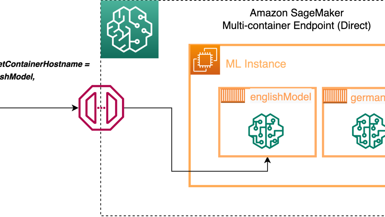
Suppose you have two models for sentiment classification, one for English language and other for German language, and these models are serving different geographies with traffic coming in at different times in a day. Instead of having two endpoints running 24/7, you can deploy both of them into one endpoint using an MCE and access them using direct invocation, thereby optimizing your resource utilization and costs. See the following code:

englishModel = {
   'Image': container1,
   'ContainerHostname': englishModel }; ...
 
germanModel = {
   'Image': container2,
   'ContainerHostname': germanModel }; ...
 
sm.create_model(
   InferenceExecutionConfig = {'Mode': 'Direct'},
   Containers = [englishModel, germanModel], ...)
sm.create_endpoint_config(EndpointConfigName = ‘my-mce-epc’,
    ProductionVariants=[{
        'InstanceType':        ‘ml.m4.xlarge’,
        'InitialInstanceCount': 2,
        'InitialVariantWeight': 1,
        'ModelName':            ‘my-multi-model-name’,
        'VariantName':          'AllTraffic'}])
sm.create_endpoint(EndpointName = ‘my-mce-endpoint’, 
                  EndpointConfigName = ‘my-mce-epc’)

In this example, we have two models (englishModel and germanModel), and we define the containers in the SageMaker create_model construct and define the InferenceExecutionConfig as ‘Direct’. Now we can call the endpoint for inference and define the TargetContainerHostname as either englishModel or germanModel depending on the client making the API call:

sm.invoke_endpoint(        
   EndpointName = endpoint_name,
   TargetContainerHostname = englishModel,
   Body = body, ...)

You can also use direct invocation within the MCE to run A/B tests to compare the performance between the models.

The following diagram illustrates our architecture.

Similarly, in other ML use cases, when the trained model is used for processing a request, the model receives data in a format that needs to be preprocessed (for example, featurized) before it can be passed to the algorithm for inference. When ML algorithms are chained together, the output of one model serves as input for the next one before reaching the final result. In this case, you can build a SageMaker MCE serial pipeline, where the containers talk to each other in the sequence defined in the create_model construct instead of you deploying each of the models into different endpoints and writing an independent logic to facilitate the flow of data between all these models and API calls. The following diagram illustrates this architecture.

For this use case, we use the following code:

sm_model = PipelineModel(name=model_name, role=aws_role, models=[Processing-1, Processing-2, Inference-1, Inference-2]) 

predictor = sm_model.deploy(initial_instance_count=1, instance_type="ml.c4.xlarge")                  
response = runtime.invoke_endpoint( 
EndpointName=predictor.endpoint,                                
    Body=body,...)

In this example, we have two processing containers (Processing-1 and Processing-2) for feature processing and data transformations, and two inference containers (Inference-1 and Inference-2) to run ML model predictions on the preprocessed data. The PipelineModel instance allows you to define the inference pipeline composed of a linear sequence of four containers that process requests for inference on data. The containers are co-located on the same instance, enabling you to run inference with low latency.

Scale multi-model endpoints for large numbers of models

The benefits of SageMaker multi-model endpoints increase based on the scale of model consolidation. You can see cost savings when hosting two models with one endpoint, and for use cases with hundreds or thousands of models, the savings are much greater.

Scaling the MCE endpoints is also straightforward using the SageMakerVariantInvocationsPerInstance predefined metric, which gives the average number of times per minute that each instance for a model endpoint is invoked to define a TargetScaling policy. SageMaker dynamically adjusts the number of instances provisioned for a model in response to changes in your workload. When the workload increases, autoscaling brings more instances online and loads with the target models and containers to keep up serving the requests. When the workload decreases, autoscaling removes unnecessary instances and offloads the model containers so that the containers don’t eat up the resources, and you don’t pay for instances that you aren’t using. The time to complete the first request against a given model experiences additional latency (called a cold start) to download the model from Amazon Simple Storage Service (Amazon S3) and load it into memory. Subsequent calls finish with no additional overhead because the model is already loaded. See the following code:

# AutoScaling client
asg = boto3.client('application-autoscaling')

# Resource type is variant and the unique identifier is the resource ID.
resource_id=f"endpoint/{endpoint_name}/variant/AllTraffic"

# scaling configuration
response = asg.register_scalable_target(
    ServiceNamespace='sagemaker', #
    ResourceId=resource_id,
    ScalableDimension='sagemaker:variant:DesiredInstanceCount', 
    MinCapacity=1,
    MaxCapacity=4
)
#Target Scaling
response = asg.put_scaling_policy(
    PolicyName=f'Request-ScalingPolicy-{endpoint_name}',
    ServiceNamespace='sagemaker',
    ResourceId=resource_id,
    ScalableDimension='sagemaker:variant:DesiredInstanceCount',
    PolicyType='TargetTrackingScaling',
    TargetTrackingScalingPolicyConfiguration={
        'TargetValue': 70.0, # Threshold
        'PredefinedMetricSpecification': {
            'PredefinedMetricType': 'SageMakerVariantInvocationsPerInstance',
        },
        'ScaleInCooldown': 300, # duration until scale in
        'ScaleOutCooldown': 60 # duration between scale out
    }
)

Following the preceding example policy configuration, we use the SageMakerVariantInvocationsPerInstance predefined metric to adjust the number of variant instances so that each instance has an InvocationsPerInstance metric of 70.

We can also scale SageMaker MCEs based on our own custom metric, such as CPUUtilization, MemoryUtilization, GPUUtilization, GPUMemoryUtilization, or DiskUtilization, to scale up or down the number of instances based on utilization of a specific resource. For more information, refer to Automatically Scale Amazon SageMaker Models.

It’s recommended that the model in each container exhibits similar compute and latency requirements on each inference request, because if traffic to the MCE shifts from a high CPU utilization model to a low CPU utilization model, but the overall call volume remains the same, the endpoint doesn’t scale out and there may not be enough instances to handle all the requests to the high CPU utilization model.

Secure MCEs

For MCEs with direct invocation, multiple containers are hosted in a single instance by sharing memory and a storage volume. It’s important to secure the containers, maintain the correct mapping of requests to target containers, and provide users with the correct access to target containers. You can restrict invoke_endpoint access to a limited set of containers inside an MCE using the sagemaker:TargetContainerHostname AWS Identity and Access Management (IAM) condition key. SageMaker uses IAM roles to provide IAM identity-based policies that you use to specify allowed or denied actions and resources and the conditions under which actions are allowed or denied. The following policies show how to limit calls to specific containers within an endpoint:

{
    "Version": "2012-10-17",
    "Statement": [
        {
            "Action": [
                "sagemaker:InvokeEndpoint"
            ],
            "Effect": "Allow",
            "Resource": "arn:aws:sagemaker:region:account-id:endpoint/endpoint_name",
            "Condition": {
                "StringLike": {
                    "sagemaker:TargetContainerHostname": ["customIps*", "common*"]
                }
            }
        }
    ]
}

Monitor multi-model endpoints using Amazon CloudWatch metrics

To make price and performance trade-offs, you’ll want to test multi-model endpoints with models and representative traffic from your own application. SageMaker provides additional metrics in Amazon CloudWatch for multi-model endpoints so you can determine the endpoint usage and the cache hit rate and optimize your endpoint. The metrics are as follows:

• ModelLoadingWaitTime – The interval of time that an invocation request waits for the target model to be downloaded or loaded to perform the inference.
• ModelUnloadingTime – The interval of time that it takes to unload the model through the container’s UnloadModel API call.
• ModelDownloadingTime – The interval of time that it takes to download the model from Amazon S3.
• ModelLoadingTime – The interval of time that it takes to load the model through the container’s LoadModel API call.
• ModelCacheHit – The number of InvokeEndpoint requests sent to the endpoint where the model was already loaded. Taking the Average statistic shows the ratio of requests in which the model was already loaded.
• LoadedModelCount – The number of models loaded in the containers in the endpoint. This metric is emitted per instance. The Average statistic with a period of 1 minute tells you the average number of models loaded per instance, and the Sum statistic tells you the total number of models loaded across all instances in the endpoint. The models that this metric tracks aren’t necessarily unique because you can load a model in multiple containers in the endpoint.

There are also several other metrics that are used by each container running on an instance, such as Invocations indicating the number of InvokeEndpoint requests sent to a container inside an endpoint, ContainerLatency giving the time an endpoint took for the target container or all the containers in a serial invocation to respond as viewed from SageMaker, and CPUUtilization and MemoryUtilizaton indicating the CPU units and percentage of memory.

Conclusion

In the post, we discussed how SageMaker multi-container endpoints can be helpful in optimizing costs and resource utilization. Examples of when to utilize MCEs include, but are not limited to, the following:

• Hosting models across different frameworks (such as TensorFlow, PyTorch, and Scikit-learn) that don’t have sufficient traffic to saturate the full capacity of an instance
• Hosting models from the same framework with different ML algorithms (such as recommendations, forecasting, or classification) and handler functions
• Comparisons of similar architectures running on different framework versions (such as TensorFlow 1.x vs. TensorFlow 2.x) for scenarios like A/B testing

SageMaker MCEs support deploying up to 15 containers on real-time endpoints and invoking them independently for low-latency inference and cost savings. The models can be completely heterogenous, with their own independent serving stack. You can either invoke these containers sequentially or independently for each request. Securely hosting multiple models, from different frameworks, on a single instance could save you up to 90% in cost compared to hosting models in dedicated single-instance endpoints.

About the authors

Dhawal Patel is a Principal Machine Learning Architect at AWS. He has worked with organizations ranging from large enterprises to mid-sized startups on problems related to distributed computing and artificial intelligence. He focuses on deep learning, including NLP and computer vision domains. He helps customers achieve high-performance model inference on Amazon SageMaker.

Vikram Elango is a Senior AI/ML Specialist Solutions Architect at Amazon Web Services, based in Virginia, US. Vikram helps global financial and insurance industry customers with design and thought leadership to build and deploy machine learning applications at scale. He is currently focused on natural language processing, responsible AI, inference optimization, and scaling ML across the enterprise. In his spare time, he enjoys traveling, hiking, cooking, and camping with his family.

Saurabh Trikande is a Senior Product Manager for Amazon SageMaker Inference. He is passionate about working with customers and is motivated by the goal of democratizing machine learning. He focuses on core challenges related to deploying complex ML applications, multi-tenant ML models, cost optimizations, and making deployment of deep learning models more accessible. In his spare time, Saurabh enjoys hiking, learning about innovative technologies, following TechCrunch, and spending time with his family.

Read More

Amazon SageMaker JumpStart provides pre-trained, open-source models for a wide range of problem types to help you get started with machine learning (ML). JumpStart also provides solution templates that set up infrastructure for common use cases, and executable example notebooks for ML with Amazon SageMaker.

As a business user, you get to do the following with JumpStart solutions:

• Explore the solutions and evaluate which are a good match for your business needs.
• Launch solutions with a single click in Amazon SageMaker Studio. This launches an AWS CloudFormation template to create the required resources.
• Modify the solution to meet your needs with access to underlying notebook and model assets.
• Delete the acquired resources once done.

This post focuses on the five ML solutions that were recently added to address five different business challenges. As of this writing, JumpStart offers 23 business solutions varying from detecting fraud in financial transactions to recognizing handwriting. The number of solutions that are offered through JumpStart increase on a regular basis as more solutions are added to it.

Solution overview

The five new solutions are as follows:

• Price optimization – Offers customizable ML models to help you make optimal decisions for setting the price of your product or service in order to achieve your business objective, such as maximizing revenue, profit, or other custom metrics.
• Bird species prediction – Shows how you can train and fine-tune an object detection model. It demonstrates model tuning through training image augmentation, and charts the accuracy improvements that occur across the iterations (epochs) of the training job.
• Lung cancer survival prediction – Shows how you can feed 2D and 3D radiomic features and patient demographics to an ML algorithm to predict a patient’s lung cancer survival chances. The results from this prediction can help providers take appropriate proactive measures.
• Financial payment classification – Demonstrates how to train and deploy an ML model to classify financial transactions based on transaction information. You can also use this solution as an intermediate step in fraud detection, personalization, or anomaly detection.
• Churn prediction for mobile phone customers – Demonstrates how to quickly develop a churn prediction model using a mobile call transaction dataset. This is a simple example for users that are new to ML.

Prerequisites

To use these solutions, make sure that you have access to Studio with an execution role that allows you to run SageMaker functionality. For your user role within Studio, make sure that the SageMaker Projects and JumpStart option is turned on.

In the following sections, we go through each of the five new solutions and discuss how it works in detail, along with some recommendations on how you can use it for your own business needs.

Price optimization

Businesses like using various levers to fetch the best results. For example, the price of a product or a service is a lever that a business can control. The question is how to decide what price to set a product or service at, in order to maximize a business objective such as profit or revenue.

This solution provides customizable ML models to help you make optimal decisions for setting the price of your product or service in order to achieve your objective, such as maximizing revenue, profit, or other custom metrics. The solution uses ML and causal inference approaches to learn price-volume relations from historical data, and is able to make dynamic price recommendations in real time to optimize the custom objective metrics.

The following screenshot shows the sample input data.

The solution includes three parts:

• Price elasticity estimation – This is estimated by causal inference via a double ML algorithm
• Volume forecast – This is forecasted using the Prophet algorithm
• Price optimization – This is achieved by a what-if simulation through different price scenarios

The solution provides the recommended price for the next day for maximizing revenue. In addition, the outputs include the estimated price elasticity, which is a value indicating the effect of price on volume, and a forecast model, which is able to forecast the next day’s volume. The following chart shows how a causal model that incorporated the calculated price elasticity performs much better under a what-if analysis (with large deviations from behavior price) than a predictive model that uses Prophet for forecasting volume using time series data.

You could apply this solution to your business for the following use cases:

• Determine the optimal price of goods for a retail store
• Estimate the effect of discount coupons on customer purchases
• Predict the effect of various incentive methods in any business

Bird species prediction

There are several computer vision (CV) applications for businesses today. One of those applications is object detection, where an ML algorithm detects the location of an object in an image by drawing a bounding box around it, and identifies the type of object it is. Learning how to apply an object detection model and fine-tune it can be of great value to an organization that has CV needs.

This solution provides an example of how to translate bounding box specifications when providing images to the SageMaker algorithm. This solution also demonstrates how to improve an object detection model by adding training images that are flipped horizontally (mirror images).

A notebook is provided for experimenting with object detection challenges when there are a large number of classes (200 bird species). The notebook also shows how to chart the accuracy improvements that occur across the epochs of the training job. The following image shows example images from the birds dataset.

This solution contains five steps:

1. Prepare the data, including download and RecordIO file generation.
2. Create and train an object detection model.
3. Deploy an endpoint and evaluate model performance.
4. Create and train an object detection model again with the expanded dataset.
5. Deploy an endpoint and evaluate the expanded model performance.

You get the following as output:

• Object detection results with bonding boxes against your test image
• A trained object detection model
• A trained object detection model with an additional expanded (flipped) dataset
• Two separate endpoints deployed with one of each model

The following chart shows model improvement against model iterations (epochs) during training.

The following examples are output from two test images.

You could apply this solution to your business for the following use cases:

• Detect objects on a conveyer belt in a packaging industry
• Detect toppings on a pizza
• Implement supply chain operational applications that involve object detection

Lung cancer survival prediction

COVID-19 brought a lot more attention to lung-related medical challenges. It has also put a lot of pressure on hospitals, doctors, nurses, and radiologists. Imagine a possibility where you can apply ML as a powerful tool to assist medical practitioners and help them speed up their work. In this solution, we show how 2D and 3D radiomic features and patient demographics can be fed to an ML algorithm to predict a patient’s lung cancer survival chances. Results from this prediction can help providers take appropriate proactive measures.

This solution demonstrates how to build a scalable ML pipeline for the Non-Small Cell Lung Cancer (NSCLC) Radiogenomics dataset, which consists of RNA sequencing data, clinical data (reflective of EHR data), and medical images. Using multiple types of data to create a machine model is referred to as multi-modal ML. This solution predicts survival outcome of patients diagnosed with non-small cell lung cancer.

The following image shows an example of the input data from the Non-Small Cell Lung Cancer (NSCLC) Radiogenomics dataset.

As part of the solution, total RNA was extracted from the tumor tissue and analyzed with RNA sequencing technology. Although the original data contains more than 22,000 genes, we keep 21 genes from 10 highly coexpressed gene clusters (metagenes) that were identified, validated in publicly available gene-expression cohorts, and correlated with prognosis.

The clinical records are stored in CSV format. Each row corresponds to a patient, and the columns contain information about the patients, including demographics, tumor stage, and survival status.

For genomic data, we keep 21 genes from 10 highly coexpressed gene clusters (metagenes) that were identified, validated in publicly available gene-expression cohorts, and correlated with prognosis.

For medical imaging data, we create patient-level 3D radiomic features that explain the size, shape, and visual attributes of the tumors observed in the CT scans. For each patient study, the following steps are performed:

1. Read the 2D DICOM slice files for both the CT scan and tumor segmentation, combine them to 3D volumes, save the volumes in NIfTI format.
2. Align CT volume and tumor segmentation so we can focus the computation inside the tumor.
3. Compute radiomic features describing the tumor region using the pyradiomics library.
4. Extract 120 radiomic features of eight classes, such as statistical representations of the distribution and co-occurrence of the intensity within tumorous region of interest, and shape-based measurements describing the tumor morphologically.

To create a multi-modal view of a patient for model training, we join the feature vectors from three modalities. We then process the data. First, we normalize the range of independent features using feature scaling. Then we perform principal component analysis (PCA) on the features to reduce the dimensionality and identify the most discriminative features that contribute 95% variance in the data.

This results in a dimensionality reduction from 215 features down to 45 principal components, which constitute features for the supervised learner.

The solution produces an ML model that predicts NSCLC patients’ survival status (dead or alive) in a form of probability. Besides the model and prediction, we also generate reports to explain the model. The medical imaging pipeline produces 3D lung CT volumes and tumor segmentation for visualization purposes.

You can apply this solution to healthcare and life sciences use cases.

Financial payment classification

Taking all financial transactions of a business or a consumer and organizing them into various categories can be quite helpful. It can help the user learn how much they have spent in which category, and it can also raise alerts when transactions or spending in a given category goes up or down unexpectedly.

This solution demonstrates how to train and deploy an ML model to classify financial transactions based on transaction information. Many banks provide this as a service to give their end-users an overview of their spending habits. You can also use this solution as an intermediate step in fraud detection, personalization, or anomaly detection. We use SageMaker to train and deploy an XGBoost model with the required underlying infrastructure.

The synthetic dataset that we to demonstrate this solution has the following features:

• transaction_category – The category of the transaction, out of the following 19 options: Uncategorized, Entertainment, Education, Shopping, Personal Care, Health and Fitness, Food and Dining, Gifts and Donations, Investments, Bills and Utilities, Auto and Transport, Travel, Fees and Charges, Business Services, Personal Services, Taxes, Gambling, Home, and Pension and insurances.
• receiver_id – An identifier for the receiving party. The identifier consists of 16 numbers.
• sender_id – An identifier for the sending party. The identifier consists of 16 numbers.
• amount – The amount that is transferred.
• timestamp – The timestamp of the transaction in YYYY-MM-DD HH:MM:SS format.

The first five observations of the dataset are as follows:

For this solution, we use XGBoost, a popular and efficient open-source implementation of the gradient boosted trees algorithm. Gradient boosting is a supervised learning algorithm that attempts to accurately predict a target variable by combining an ensemble of estimates from a set of simpler and weaker models. Its implementation is available in the SageMaker built-in algorithms.

The financial payment classification solution contains four steps:

1. Prepare the data.
2. Build a feature store.
3. Create and train an XGBoost model.
4. Deploy an endpoint and evaluate model performance.

We get the following output:

• A trained XGBoost model based on our example dataset
• A SageMaker endpoint that can predict the transaction category

After running this solution, you should see a classification report similar to the following.

Possible applications for your business include the following:

• Various financial applications in retail and investment banking
• When transactions need to be classified in any use case (not just financial)

Churn prediction for mobile phone customers

Predicting customer churn is a very common business need. Numerous studies show that the cost of retaining an existing customer is much less than acquiring a new customer. The challenge often comes from businesses having a tough time understanding why a customer is churning, or building a model that predicts churning.

In this example, users that are new to ML can experience how a churn prediction model can be quickly developed using a mobile call transaction dataset. This solution uses SageMaker to train and deploy an XGBoost model on a customer profile dataset to predict whether a customer is likely to leave a mobile phone operator.

The dataset this solution uses is publicly available and is mentioned in the book Discovering Knowledge in Data by Daniel T. Larose. It is attributed by the author to the University of California Irvine Repository of Machine Learning Datasets.

This dataset uses the following 21 attributes to describe the profile of a customer of an unknown US mobile operator.

• State: the US state in which the customer resides, indicated by a two-letter abbreviation; for example, OH or NJ
• Account Length: the number of days that this account has been active
• Area Code: the three-digit area code of the corresponding customer’s phone number
• Phone: the remaining seven-digit phone number
• Int’l Plan: whether the customer has an international calling plan: yes/no
• VMail Plan: whether the customer has a voice mail feature: yes/no
• VMail Message: the average number of voice mail messages per month
• Day Mins: the total number of calling minutes used during the day
• Day Calls: the total number of calls placed during the day
• Day Charge: the billed cost of daytime calls
• Eve Mins, Eve Calls, Eve Charge: the billed cost for calls placed during the evening
• Night Mins, Night Calls, Night Charge: the billed cost for calls placed during nighttime
• Intl Mins, Intl Calls, Intl Charge: the billed cost for international calls
• CustServ Calls: the number of calls placed to Customer Service
• Churn?: whether the customer left the service: true/false

This solution contains three stages:

1. Prepare the data.
2. Create and train an XGBoost model.
3. Deploy an endpoint and evaluate model performance.

We get the following output:

• A trained XGBoost model based on our example dataset to predict user churn
• A SageMaker endpoint that can predict user churn

This model helps estimate how many of the 5,000 mobile phone customers are likely to stop using their current mobile phone operator.

The following chart shows a probability distribution of the churn as an output from the model.

You could apply this to your business for the following use cases:

• Predict customer churn in your own business
• Classify which customers may open your marketing email and who will not (binary classification)
• Predict which students are likely to drop out from a course

Clean up resources

After you’re done running a solution in JumpStart, make sure to choose Delete all resources so all the resources that you have created in the process are deleted and your billing is stopped.

Summary

This post showed you how to solve various business problems by applying ML, based on JumpStart solutions. Although this post focused on the five new solutions that were recently added to JumpStart, there are a total of 23 available solutions. We encourage you to log in to Studio and look at the JumpStart solutions yourselves and start deriving immediate value out of them. For more information, refer to Amazon SageMaker Studio and SageMaker JumpStart.

Note: If you don’t see all of the above five solutions in the JumpStart console of your AWS region, please wait for a week and check again. We are releasing them to various regions in a phased manner.

About the Authors

Dr. Raju Penmatcha is an AI/ML Specialist Solutions Architect in AI Platforms at AWS. He works on the low-code/no-code suite of services in SageMaker that help customers easily build and deploy machine learning models and solutions. When not helping customers, he likes traveling to new places.

Manan Shah is a Software Development Manager at Amazon Web Services. He is an ML enthusiast and focuses on building no-code/low-code AI/ML products. He strives to empower other talented, technical people to build great software.

Read More

In the pursuit of superior accuracy, deep learning models in areas such as natural language processing and computer vision have significantly grown in size in the past few years, frequently counted in tens to hundreds of billions of parameters. Training these gigantic models is challenging and requires complex distribution strategies. Data scientists and machine learning engineers are constantly looking for the best way to optimize their training compute, yet are struggling with the communication overhead that can increase along with the overall cluster size.

This is why we recently launched sharded data parallelism on Amazon SageMaker, a new memory-saving distributed training technique in the SageMaker model parallel (SMP) library. Sharded data parallelism is purpose-built for extreme-scale models and uses Amazon in-house MiCS technology under the hood, a science effort to minimize the communication scale by bringing down expensive communication overhead rooted in parameter gathering and gradient synchronization. With a 30B parameter GPT-2 model with sequence length 2048, this new feature achieved 141 TFLOPs, a 39.7% speed up compared to DeepSpeed ZeRO-3. For a 10B GPT-2 model with sequence length 512, this new feature also achieved 564 samples per second, a 13.9% speed up compared to PyTorch’s Fully Sharded Data Parallel (FSDP). Remember that in gigantic model training, every percentage of speedup translates to dollars saved and productivity gained in your team.

In this blog post, we’ll first take a closer look at the key differentiators of sharded data parallelism and when to use it. Then, you’ll learn how to train a 30B parameter GPT-2 model on SageMaker with ease with this new feature. Finally we’ll compare the performance with other open source options, notably outperforming DeepSpeed ZeRO by up to 39.7% on 256 GPUs.

How sharded data parallelism works and when to use it

Before we introduce sharded data parallelism, let’s look at its broader technique family. Recent distributed training approaches for large models have moved to a paradigm where model parameters, gradients, and optimizer states are shared across data-parallel nodes. Unlike Pipeline Parallelism which has the innate complexity of choosing layers to partition across devices especially when your framework doesn’t support automated model splitting, this paradigm elegantly preserves the simplicity of data parallelism, while removing data parallelism’s constraint where a model must fit into a single GPU.

In existing frameworks that fall under this paradigm, notably DeepSpeed ZeRO-3 and PyTorch’s FSDP upstreamed from FairScale, model states are sharded across all GPUs, a strategy that lowers the memory consumption on each GPU at the cost of incurring large communication overhead which increases with cluster size and therefore causes the scalability to significantly drop at scale. In contrast, sharded data parallelism in the SMP library partitions model states in a scale-aware manner by partitioning each replica of model states only within a subset of GPUs.

Let’s look closer at the scale-aware model partitioning in MiCS, the core technology behind sharded data parallel. The intuition behind this design is that partitioning training states across the entire data-parallel group may not be required to train a model with tens of billions of parameters. For example, 8 V100 GPUs (32GB each) are sufficient to hold the model states replica of a 10B-parameter model which needs about 200GB of memory when training with Adam optimizer using mixed-precision. By limiting a complete replica of model states in the smallest subset of GPUs, we can effectively reduce the scale of communication overhead compared to DeepSpeed and PyTorch FSDP. Sharded data parallel also leverages other techniques in MiCS such as Hierarchical Communication and 2-hop Gradient Synchronization. For more information, check out Near-linear scaling of gigantic-model training on AWS or MiCS: Near-linear Scaling for Training Gigantic Model on Public Cloud.

Now, how do you know when to choose sharded data parallel over other distributed training techniques? The general rule is that if your model has less than 1 billion parameters and can fit into GPU memory, SageMaker data parallel library or SageMaker training compiler can be sufficient for you. If you have larger language or computer vision models, our suggestion is to train it with the sharded data parallelism technique combined with activation checkpointing and activation offloading in the SageMaker model parallel library first, before other techniques such as tensor parallelism or pipeline parallelism.

Using sharded data parallelism to train GPT-2 on Amazon SageMaker

Let’s now learn how to train a GPT-2 model with sharded data parallel, with SMP encapsulating the complexity for you. This complete tutorial notebook walks you through the entire process, from data processing, defining and submitting training jobs, to monitoring training logs. What follows is a brief overview highlighting key steps for using this feature.

1. Get started

Sharded data parallelism is available in PyTorch v1.12.0+ and works with both FP16 and BF16. The easiest way to use the SMP library is through a prebuilt AWS Deep Learning Container for PyTorch. However, if you want to bring your own Docker container, you can refer to Create Your Own Docker Container with the SageMaker Distributed Model Parallel Library. To get started, follow Modify a PyTorch Training Script to adapt SMPs’ APIs in your training script. In this section, we only call out a few main steps with code snippets from the ready-to-use training script train_gpt_simple.py. You can follow the comments in the script and API document to learn more about where SMP APIs are used.

First, import and initialize the library by calling smdistributed.modelparallel.torch.init() at the beginning of the training script:

import smdistributed.modelparallel.torch as smp

smp.init(smp_config)

Second, wrap the model to be partitioned with smdistributed.modelparallel.torch.DistributedModel and use the returned DistributedModel object going forward:

from transformers import AutoModelForCausalLM

model = AutoModelForCausalLM.from_config(model_config)
model = smp.DistributedModel(model, trace_device="gpu", backward_passes_per_step=args.gradient_accumulation)

Wrap the optimizer with smdistributed.modelparallel.torch.DistributedOptimizer for saving and loading optimizer states.

from torch import optim

optimizer = optim.Adam(
    param_groups, betas=(args.beta1, args.beta2), lr=args.lr, weight_decay=args.weight_decay
)

optimizer = smp.DistributedOptimizer(
        optimizer, 
        static_loss_scale=None, 
        dynamic_loss_scale=True,
        dynamic_loss_args={"scale_window": 1000, "min_scale": 1, "delayed_shift": 2},
        )

Put the forward and backward logic in a step function and decorate it with smdistributed.modelparallel.torch.step.  Any computation defined inside the smp.step-decorated function is executed in a distributed manner.

@smp.step
def train_step(model, optimizer, input_ids, attention_mask, args):
    loss = model(input_ids=input_ids, attention_mask=attention_mask, labels=input_ids)["loss"]
    model.backward(loss)

    return loss

@smp.step
def test_step(model, input_ids, attention_mask):
    loss = model(input_ids=input_ids, attention_mask=attention_mask, labels=input_ids)["loss"]
    
    return loss

2. Prepare the dataset

We use the openwebtext is the dataset we use in this example. The notebook uses the script data_prep_512.py to download and preprocess the dataset. You can also train with other datasets by modifying data_pipeline.py. When dealing with large dataset and model, you can speed up the training job by using data stored in Amazon FSx for Lustre, which provides a high-performance file system natively integrated with Amazon Simple Storage Service (S3). Please see the instructions from Configure Data Input Channel to Use Amazon FSx for Lustre for guidance on setting an FSx Lustre file system as data input channel.

3. Start the training jobs

This step assumes you have already modified your training script and prepared the dataset as mentioned in the preceding sections. To enable sharded data parallelism, simply set the sharded_data_parallel_degree in the PyTorch Estimator. In this tutorial, we set sharded_data_parallel_degree=128 and instace_count=32 for p4d.24xlarge nodes, which indicates that the model states will be sharded across 128 GPUs among the total 256 GPUs. Based on this selected value, SMP will then automatically sets the data parallel degree to 2 (because 256/128=2), meaning we’ll have two replicas for data parallelism. A general rule for picking an ideal value for sharded_data_parallel_degree is to add one more node to the sharing group per every 3B of model parameters. In this tutorial, our model size is 30B, so we should use at least 10 nodes for sharding. And because 16 nodes (128 GPUs) is the smallest power-of-2 above the threshold, we set sharded_data_parallel_degree=128.

For checkpointing, we also provide a set of checkpointing utilities in sharded_data_parallel_checkpoint.py , including a utility to reconstruct the full state_dict for advanced use cases. Finally, we can launch a distributed training job by calling fit() on the Estimator.

smp_estimator = PyTorch(
    entry_point="train_gpt_simple.py",
    instance_type="ml.p4d.24xlarge",
    source_dir=os.getcwd(),
    volume_size=500,
    instance_count=32,
    distribution={
        "mpi": {
            "enabled": True,
            "processes_per_host": processes_per_host,
            "custom_mpi_options": mpioptions,
        },
        "smdistributed": {
            "modelparallel": {
                "enabled": True,
                "parameters": {
                    "ddp": True,
                    "skip_tracing": True,
                    "delayed_parameter_initialization": True,
                    "offload_activations": True,
                    "activation_loading_horizon": 4,
                    # To enable sharded data parallelism.
                    # Here we shard model states across 128 GPUs. 
                    "sharded_data_parallel_degree": 128, 
                    "fp16": False,
                    "bf16": True,
                    # This is to disable pipeline parallelism.
                    "partitions": 1,
                },
            }
        },
    },
    framework_version="1.12",
    py_version="py38",
    hyperparameters=hyperparameters,
    checkpoint_s3_uri=checkpoint_s3_uri if not use_fsx else None,
    checkpoint_local_path=hyperparameters["checkpoint-dir"] if use_fsx else None,
    ...
)

smp_estimator.fit(inputs=data_channels)

4. Monitor the training jobs

You can access the training logs and track GPU and memory utilization on Amazon CloudWatch. Make sure to look at the logs of “algo-1” because that is the main node whose output stream has the training job logs from all instances.

Benchmarking performance

We benchmarked sharded data parallelism in the SMP library on both 16 and 32 p4d.24xlarge nodes for sequence length 512 and 2048, respectively. The 30B-parameter GPT2 model is configured to use a hidden width of 7168, 48 layers, and 64 heads. You can adopt the exact same configuration where sequence length is 2048 by setting model_config = "gpt2-30b" in the tutorial notebook. With this setting, SMP achieved 73.52 samples per second, a 39.7% speed up compared to DeepSpeed ZeRO-3. If your token size is 500 billion, this speed up means nearly 367 hours of savings on p4d.24xlarge nodes, an equivalent of more than $12,000 budget saved per training! The following table summarizes our benchmark results.

1/ For each model configuration, we tested different features, stages, and configurations in DeepSpeed ZeRO and chose the one that provides the best throughput as the DeepSpeed baseline. The benchmark was run on Amazon Elastic Compute Cloud (Amazon EC2). 2/ These results rely on improved communication collectives optimized for AWS which will be made available soon. 3/ Time to train is projected from speed based on number of tokens processed.

In summary, we observed consistently higher throughput with sharded data parallelism in SMP when compared to DeepSpeed across a range of models and configurations. This new feature also demonstrated a better memory efficiency compared to DeepSpeed, enabling SMP to fit a larger batch size and reduce the level of gradient accumulation required to fit a particular global batch size.

Conclusion

In this post, we introduced a new distributed training technique — sharded data parallelism — and how it speeds up gigantic model training with near linear-scaling on Amazon SageMaker. We also walked through how to train a GPT-2 model with the new technique following this complete example. You can follow the Amazon SageMaker Examples GitHub repo to track all SageMaker model parallel examples or attend our next distributed training workshops. To learn more about sharded data parallelism, please see the documentation.

About the authors

Emily Webber joined AWS just after SageMaker launched, and has been trying to tell the world about it ever since! Outside of building new ML experiences for customers, Emily enjoys meditating and studying Tibetan Buddhism.

Can Karakus is a Senior Applied Scientist at AWS, optimizing large-scale distributed deep learning on AWS. His research interests cover deep learning, distributed optimization, distributed systems, and information theory. Outside of work, he enjoys cycling, traveling, reading and learning.

Rahul Huilgol is a Senior Software Engineer at AWS. He works on distributed deep learning systems, towards making it easy and performant to train large deep learning models in the cloud. In his spare time, he enjoys photography, biking and gardening.

Suhit Kodgule is a Software Development Engineer with AWS Artificial Intelligence group working on deep learning frameworks. In his spare time, he enjoys hiking, traveling and cooking.

Erin Ho is a Product Manager for AWS Deep Learning. She works on products that make it easier for customers to train deep learning models on AWS. For fun outside work, she enjoys hiking and skiing.

Read More