Using different levels of precision for different arithmetic tasks reduces computational burden without compromising performance.Read More

Rock ‘n’ Robotics: The White Stripes’ AI-Assisted Visual Symphony
Playfully blending art and technology, underground animator Michael Wartella has teamed up with artificial intelligence to breathe new life into The White Stripes’ fan-favorite song, “Black Math.”
The video was released earlier this month to celebrate the 20th anniversary of the groundbreaking “Elephant” album.
Wartella is known for his genre-bending work as a cartoonist and animator.
His Brooklyn-based Dream Factory Animation studio produced the “Black Math” video, which combines digital and practical animation techniques with AI-generated imagery.
“This track is 20 years old, so we wanted to give it a fresh look, but we wanted it to look like it was cut from the same cloth as classic White Stripes videos,” Wartella said.
For the “Black Math” video, Wartella turned to Automatic1111, an open-source generative AI tool. To create the video, Wartella and his team started off with the actual album cover, using AI to “bore” into the image.
They then used AI to train the AI and build more images in a similar style. “That was really crazy and interesting and everything built from there,” Wartella said.
This image-to-image deep learning model caused a sensation on its release last year, and is part of a new generation of AI tools that are transforming the arts.
“We used several different AI tools and animation tools,” Wartella said. “For every shot, I wanted this to look like an AI video in a way those classic CGI videos look very CGI now.”
Wartella and his team relied heavily on archived images and video of the musician duo as well as motion-capture techniques to create a video replicating the feel of late-1990s and early-2000s music videos.
Wartella has long relied on NVIDIA GPUs to run a full complement of digital animation tools on workstations from Austin, Texas-based BOXX Technologies.
“We’ve used BOXX workstations with NVIDIA cards for almost 20 years now,” he said. “That combination is just really powerful — it’s fast, it’s stable.”
Wartella describes his work on the “Black Math” video as a “collaboration” with the AI tool, using it to generate images, tweaking the results and then returning to the technology for more.
“I see this as a collaboration, not just pressing a button. It’s an incredibly creative tool,” Wartella said of generative AI.
The results were sometimes “kind of strange,” a quality that Wartella prizes.
He took the output from the AI, ran it through conventional composition and editing tools, and then processed the results through AI again.
Wartella felt that working with AI in this way made the video stronger and more abstract.

The video presents Jack and Meg White in their 2003 personas, emerging from a whimsical, dark cyber fantasy.
The video parallels the look and feel of the band’s videos from the early 2000s, even as it leans into the otherworldly, almost kaleidoscopic qualities of modern generative AI.
“The lyrics are anti-authoritarian and punkish, so the sound steered this one in the direction,” Wartella said. “The song itself has a scientific theme that is already a perfect fit for the AI.”
When “Black Math” was first released as part of The White Stripes’ critically acclaimed “Elephant” album, it grabbed attention for its high-energy, powerful guitar riffs and Jack White’s unmistakable vocals.
The song played a role in cementing the band’s reputation as a critical player in the garage rock revival of the early 2000s.
Wartella’s inventive approach with “Black Math” highlights the growing use of AI — as well as lively discussion of its implications — among creatives.
Over the past few months, AI-generated art has been increasingly prevalent across various social media platforms, thanks to tools like Midjourney, OpenAI’s Dall·E, DreamStudio and Stable Diffusion.
As AI advances, Wartella said, we can expect to see more artists exploring the potential of these tools in their work.
“I’m in full favor of people having the opportunity to play around with the technology,” Wartella said. “We’ll definitely use AI again if the song or the project calls for it.”
The release of the “Black Math” music video coincides with the launch of “The White Stripes Elephant (20th Anniversary)” deluxe vinyl reissue package, available now through Jack White’s Third Man Records and Sony Legacy Recordings.
Watch the “Black Math” music video:

Serving With TF and GKE: Stable Diffusion

Posted by Chansung Park and Sayak Paul (ML and Cloud GDEs)
Generative AI models like Stable Diffusion1 that lets anyone generate high-quality images from natural language text prompts enable different use cases across different industries. These types of models allow people to generate these images not only from images but also condition them with other inputs such as segmentation maps, other images, depth maps, etc. In many ways, an end Stable Diffusion system (such as this) is often very complete. One gives a free-form text prompt to start the generation process, and in the end, an image (or any data in the continuous modality) gets generated.
In this post, we discuss how TensorFlow Serving (TF Serving) and Google Kubernetes Engine (GKE) can serve such a system with online deployment. Stable Diffusion is just one example of many such systems that TF and GKE can serve with online deployment. We start by breaking down Stable Diffusion into main components and how they influence the subsequent consideration for deployment. Then we dive deep into the deployment-specific bits such as TF Serving deployment and k8s cluster configuration. Our code is open-sourced in this repository.
Let’s dive in.
Stable Diffusion in a nutshell
Stable Diffusion, is comprised of three sub-models:
- CLIP’s text tower as the Text Encoder,
- Diffusion Model (UNet), and
- Decoder of a Variational Autoencoder
When generating images from an input text prompt, the prompt is first embedded into a latent space with the text encoder. Then an initial noise is sampled, which is fed to the Diffusion model along with the text embeddings. This noise is then denoised using the Diffusion model in a continuous manner – the so-called “diffusion” process. The output of this step is a denoise latent, and it is fed to the Decoder for final image generation. Figure 1 provides an overview.
(For a more complete overview of Stable Diffusion, refer to this post.)
 |
| Figure 1. Stable Diffusion Architecture |
As mentioned above, three sub-models of Stable Diffusion work in a sequential manner. It’s common to run all three models on a single server (which constructs the end Stable Diffusion system) and serve the system as a whole.
However, because each component is a standalone deep learning model, each one could be served independently. This is particularly useful because each component has different hardware requirements. This can also have potentially improved resource utilization. The text encoder can still be run on moderate CPUs, whereas the other two should be run on GPUs, especially the UNet should be served with larger size GPUs (~3.4 GBs in size).
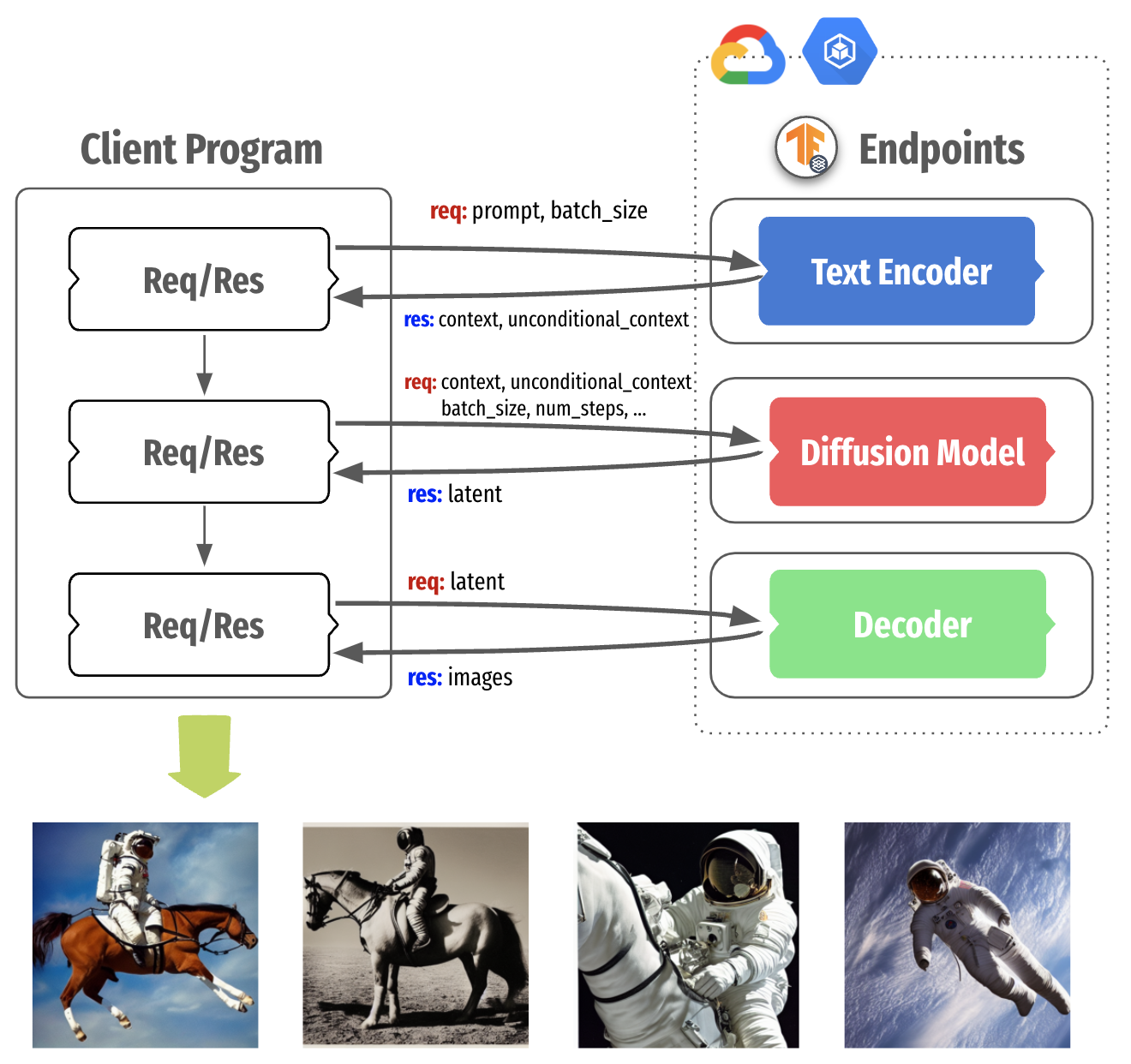 |
| Figure 2. Decomposing Stable Diffusion in three parts |
Figure 2 shows the Stable Diffusion serving architecture that packages each component into a separate container with TensorFlow Serving, which runs on the GKE cluster. This separation brings more control when we think about local compute power and the nature of fine-tuning of Stable Diffusion as shown in Figure 3.
NOTE: TensorFlow Serving is a flexible, high-performance serving system for machine learning models, designed for production environments, which is widely adopted in industry. The benefits of using it include GPU serving support, dynamic batching, model versioning, RESTful and gRPC APIs, to name but a few.
In modern personal devices such as desktops and mobile phones, it is common that they are equipped with moderate CPUs and sometimes GPU/NPUs. In this case, we could selectively run the UNet and/or Decoder in the cloud using high capacity GPUs while running the text encoder locally on the user’s device. In general, this approach allows us to flexibly architect the Stable Diffusion system in a way to maximize the resource utilization.
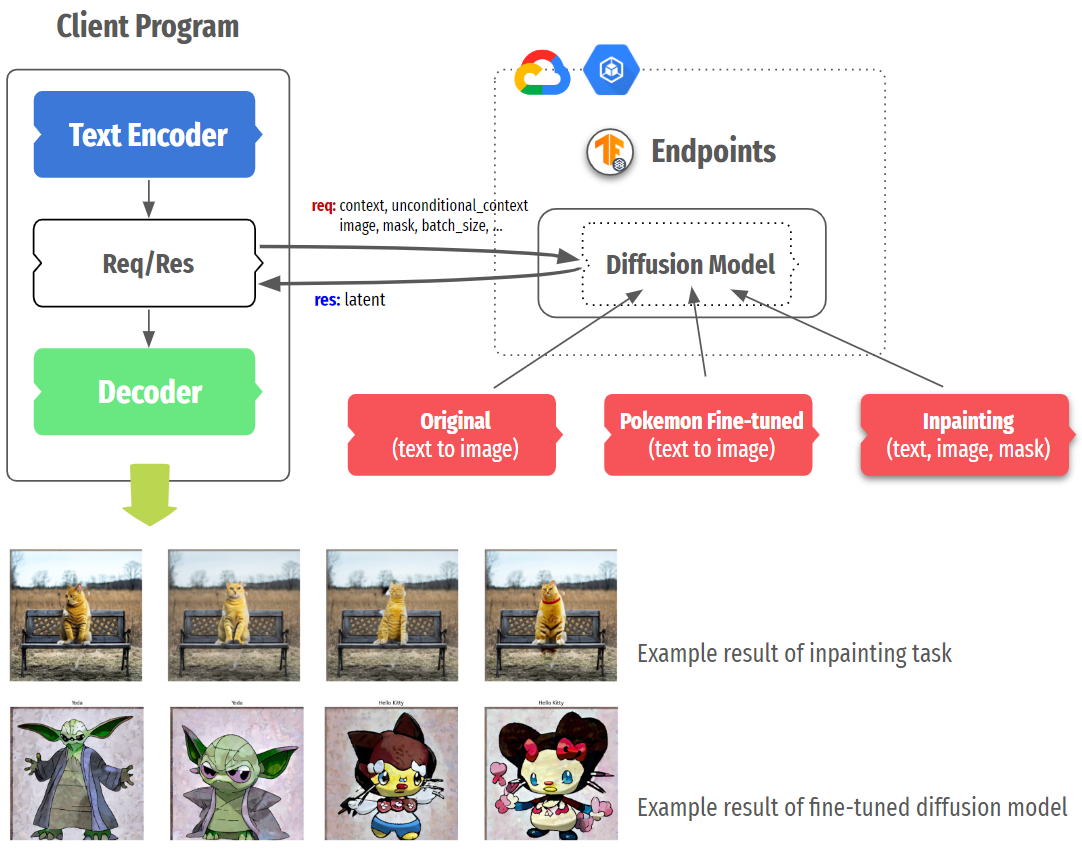 |
| Figure 3. Flexible serving structure of Stable Diffusion |
One more scenario to consider is fine-tuned Stable Diffusion. Many variations such as DreamBooth, Textual Inversion, or style transfer have shown that modifying only one or two components (usually Text Encoder and UNet) can generate images with new concepts or different styles. In this case, we could selectively deploy more of certain fine-tuned models on separate instances or replace existing models without touching other parts.
Wrapping Stable Diffusion in SavedModels
In order to serve a TensorFlow/Keras model with TF Serving, it should be saved in the SavedModel format. After that, the model can be served by TF Serving, a high-performance serving system for machine learning models, specially designed for production environments. The potentially non-trivial parts of making a SavedModel could be divided into three parts:
- defining an appropriate input signature specification of the underlying model,
- performing computations with the underlying model so that everything can be compiled in native TensorFlow, and
- including most of the pre and post-processing operations within the
SavedModelgraph itself to reduce training/serving skew (this is optional, but highly recommended).
To make the Stable Diffusion class shipped in KerasCV compatible with TF Serving, we need to first isolate the sub-networks (as mentioned above) of the class. Recall that we have got three sub-networks here: text encoder, diffusion model, and a decoder. We then have to serialize these networks as SavedModels.
A diffusion system also involves iterative sampling where a noise vector is gradually turned into an image. KerasCV’s Stable Diffusion class implements the sampling process with non-TensorFlow operations. So, we need to eliminate those operations and ensure that it’s implemented in pure TensorFlow so that there is end-to-end compatibility. This was the single most challenging aspect for us in the whole project.
Since the serialization of the text encoder and the decoder is straightforward, we’ll skip that in this post and instead, focus on the serialization of the diffusion model, including the sampling process. You can find an end-to-end notebook here.
Diffusion Model and Iterative Sampling
We start by defining an input signature dictionary for the SavedModel to be serialized. In this case, the inputs consist:
context, that denotes embeddings of the input text prompt extracted with the text encoderunconditional_context, that denotes the embeddings of a so-called “null prompt” (see classifier-free guidance)num_steps, that denotes the number of sampling steps for the reverse diffusion processbatch_size, that denotes the number of images to be returned
from keras_cv.models.stable_diffusion.constants import ALPHAS_CUMPROD_TF |
Next up, we implement the iterative reverse diffusion process that involves the pre-trained diffusion model. diffusion_model_exporter() takes this model as an argument. serving_fn() is the function we use for exporting the final SavedModel. Most of this code is taken from the original KerasCV implementation here, except it has got all the operations implemented in native TensorFlow.
def diffusion_model_exporter(model: tf.keras.Model): |
Then, we can serialize the diffusion model as a SavedModel like so:
tf.saved_model.save( |
Here, diffusion_model is the pre-trained diffusion model initialized like so:
from keras_cv.models.stable_diffusion.diffusion_model import DiffusionModel |
Deploy Stable Diffusion to GKE
Once you have successfully created TensorFlow SavedModels, it is quite straightforward to deploy them with TensorFlow Serving to a GKE cluster in the following steps.
- Write Dockerfiles which are based on the TensorFlow Serving base image
- Create a GKE cluster with accelerators attached
- Apply NVIDIA GPU driver installation daemon to install the driver on each node
- Write deployment manifests with GPU allocation
- Write service manifests to expose the deployments
- Apply all the manifests
The easiest way to wrap a SavedModel in TensorFlow Serving is to leverage the pre-built TensorFlow Serving Docker images. Depending on the configuration of the machine that you’re deploying to, you should choose either tensorflow/serving:latest or tensorflow/serving:latest-gpu. Because all the steps besides GPU-specific configuration are the same, we will explain this section with an example of the Diffusion Model part only.
By default, TensorFlow Serving recognizes embedded models under /models, so the entire SavedModel folder tree should be placed inside /models/{model_name}/{version_num}. A single TensorFlow Serving instance can serve multiple versions of multiple models, so that is why we need such a {model_name}/{version_num} folder structure. A SavedModel can be exposed as an API by setting a special environment variable MODEL_NAME, which is used for TensorFlow Serving to look for which model to serve.
FROM tensorflow/serving:latest-gpu |
Next step is to create a GKE cluster. You can do this by using either Google Cloud Console or gcloud container CLI as below. If you want accelerators available on each node, you can specify how many of which GPUs to be attached with --accelerator=type={ACCEL_TYPE}, count={ACCEL_NUM} option.
$ gcloud container clusters create {CLUSTER_NAME} |
Once the cluster is successfully created, and if the nodes in the cluster have accelerators attached, an appropriate driver for them should be installed correctly. This is done by running a special DaemonSet, which tries to install the driver on each node. If the driver has not been successfully installed, and if you try to apply Deployment manifests requiring accelerators, the status of the pod remains as Pending.
DRIVER_URL = https://raw.githubusercontent.com/GoogleCloudPlatform/container-engine-accelerators/master/nvidia-driver-installer/cos/daemonset-preloaded.yaml |
Make sure all the pods are up and running with kubectl get pods -A command. Then, we are ready to apply prepared Deployment manifests. Below is an example of the Deployment manifest for the Diffusion Model. The only consideration you need to take is to specify which resource the pods of the Deployment should consume. Because the Diffusion Model needs to be run on accelerators, resources:limits:nvidia.com/gpu: {ACCEL_NUM} should be set.
Furthermore, if you want to expose gRPC and RestAPI at the same time, you need to set containerPort for both. TensorFlow Serving exposes the two endpoints via 8500 and 8501, respectively, by default, so both ports should be specified.
apiVersion: apps/v1 |
One more thing to note is that --rest_api_timeout_in_ms flag is set in args with a huge number. It takes a long time for heavy models to run inference. Since the flag is set to 5,000ms by default which is 5 seconds, sometimes timeout occurs before the inference is done. You can experimentally find out the right number, but we simply set this with a high enough number to demonstrate this project smoothly.
The final step is to apply prepared manifest files to the provisioned GKE cluster. This could be easily done with the kubectl apply -f command. Also, you could apply Service and Ingress depending on your needs. Because we simply used vanilla LoadBalancer type of Service for demonstration purposes, it is not listed in this blog. You can find all the Dockerfiles, and the Deployment and Service manifests in the accompanying GitHub repository.
Let’s generate images!
Once all the TensorFlow Serving instances are deployed, we could generate images by calling their endpoints. We will show how to do it through RestAPI, but you could do the same with the gRPC channel as well. The image generation process could be done in the following steps:
- Prepare tokens for the prompt of your choice
- Send the tokens to the Text Encoder endpoint
- Send context and unconditional context obtained from the Text Encoder to the Diffusion Model endpoint
- Send latent obtained from the Diffusion Model to the Decoder endpoint
- Plot the generated images
Since it is non-trivial to embed a tokenizer into the Text Encoder itself, we need to prepare the tokens for the prompt of your choice. KerasCV library provides SimpleTokenizer in the keras_cv.models.stable_diffusion.clip_tokenizer module, so you could simply pass the prompt to it. Since the Diffusion Model is designed to accept 77 tokens, the tokens are padded with MAX_PROMPT_LENGTH up to 77 long.
NOTE: Since KerasCV comes with lots of modules that we don’t need for tokenization, it is not recommended to import the entire library. Instead, you could simply copy the codes for the SimpleTokenizer in your environment. Due to incompatibility issues, the current tokenizer cannot be shipped as a part of the Text Encoder SavedModel.
from keras_cv.models.stable_diffusion.clip_tokenizer import SimpleTokenizer
|
Once the tokens are prepared, we could simply pass it to the Diffusion Model’s endpoint. The headers and the way to call the all endpoints are identical as below, so we will omit it in the following steps. Just keep in mind you set the ADDRESS and the MODEL_NAME correctly, which is identical to the one we set in each Dockerfile.
import requests
|
As you see, each payload is dependent on the upstream tasks. For instance, we pass tokens to the Text Encoder’s endpoint, context and unconditional_context retrieved from the Text Encoder to the Diffusion Model’s endpoint, and latent retrieved from the Diffusion Model to Decoder’s endpoint. The signature_name should be the same as when we created SavedModel with the signatures argument.
import json
|
The final response from the Decoder’s endpoint contains a full of pixel values in a list, so we need to convert those into a format that the environment of your choice could understand as images. For demonstration purposes, we used the tf.convert_to_tensor() utility function that turns the Python list into TensorFlow’s Tensor. However, you could plot the images in different languages, too, with your most familiar methods.
import matplotlib.pyplot as plt
|
 |
| Figure 4. Generated images with three TensorFlow Serving endpoints |
Note on XLA compilation
We can obtain a speed-up of 17 – 25% by incorporating compiling the SavedModels to be XLA compatible. Note that the individual sub-networks of the Stable Diffusion class are fully XLA compatible. But in our case, the SavedModels also contain important operations that are in native TensorFlow, such as the reverse diffusion process.
For deployment purposes, this speed-up could be impactful. To know more, check out the following repository: https://github.com/sayakpaul/xla-benchmark-sd.
Conclusion
In this blog post, we explored what Stable Diffusion is, how it could be decomposed into the Text Encoder, Diffusion Model, and Decoder, and why it might be beneficial for better resource utilization. Also, we touched upon the concrete demonstration about the deployment of the decomposed Stable Diffusion by creating SavedModels, containerizing them in TensorFlow Serving, deploying them on the GKE cluster, and running image generations. We used the vanilla Stable Diffusion, but feel free to try out replacing the only Diffusion Model with in-painting or pokemon fine-tuned diffusion models.
References
CLIP: Connecting text and images, OpenAI, https://openai.com/research/clip.
The Illustrated Stable Diffusion, Jay Alammar, https://jalammar.github.io/illustrated-stable-diffusion/.
Stable Diffusion, Stability AI, https://stability.ai/stable-diffusion.
Acknowledgements
We are grateful to the ML Developer Programs team that provided Google Cloud credits to support our experiments. We thank Robert Crowe for providing us with helpful feedback and guidance.
___________
1 Stable Diffusion is not owned or operated by Google. It is made available by Stability AI. Please see their site for more information: https://stability.ai/blog/stable-diffusion-public-release.Read More
Improved Speech Recognition for People Who Stutter
Apple Machine Learning Research

An ML-based approach to better characterize lung diseases
The combination of the environment an individual experiences and their genetic predispositions determines the majority of their risk for various diseases. Large national efforts, such as the UK Biobank, have created large, public resources to better understand the links between environment, genetics, and disease. This has the potential to help individuals better understand how to stay healthy, clinicians to treat illnesses, and scientists to develop new medicines.
One challenge in this process is how we make sense of the vast amount of clinical measurements — the UK Biobank has many petabytes of imaging, metabolic tests, and medical records spanning 500,000 individuals. To best use this data, we need to be able to represent the information present as succinct, informative labels about meaningful diseases and traits, a process called phenotyping. That is where we can use the ability of ML models to pick up on subtle intricate patterns in large amounts of data.
We’ve previously demonstrated the ability to use ML models to quickly phenotype at scale for retinal diseases. Nonetheless, these models were trained using labels from clinician judgment, and access to clinical-grade labels is a limiting factor due to the time and expense needed to create them.
In “Inference of chronic obstructive pulmonary disease with deep learning on raw spirograms identifies new genetic loci and improves risk models”, published in Nature Genetics, we’re excited to highlight a method for training accurate ML models for genetic discovery of diseases, even when using noisy and unreliable labels. We demonstrate the ability to train ML models that can phenotype directly from raw clinical measurement and unreliable medical record information. This reduced reliance on medical domain experts for labeling greatly expands the range of applications for our technique to a panoply of diseases and has the potential to improve their prevention, diagnosis, and treatment. We showcase this method with ML models that can better characterize lung function and chronic obstructive pulmonary disease (COPD). Additionally, we show the usefulness of these models by demonstrating a better ability to identify genetic variants associated with COPD, improved understanding of the biology behind the disease, and successful prediction of outcomes associated with COPD.
ML for deeper understanding of exhalation
For this demonstration, we focused on COPD, the third leading cause of worldwide death in 2019, in which airway inflammation and impeded airflow can progressively reduce lung function. Lung function for COPD and other diseases is measured by recording an individual’s exhalation volume over time (the record is called a spirogram; see an example below). Although there are guidelines (called GOLD) for determining COPD status from exhalation, these use only a few, specific data points in the curve and apply fixed thresholds to those values. Much of the rich data from these spirograms is discarded in this analysis of lung function.
We reasoned that ML models trained to classify spirograms would be able to use the rich data present more completely and result in more accurate and comprehensive measures of lung function and disease, similar to what we have seen in other classification tasks like mammography or histology. We trained ML models to predict whether an individual has COPD using the full spirograms as inputs.
 |
| Spirometry and COPD status overview. Spirograms from lung function test showing a forced expiratory volume-time spirogram (left), a forced expiratory flow-time spirogram (middle), and an interpolated forced expiratory flow-volume spirogram (right). The profile of individuals w/o COPD is different. |
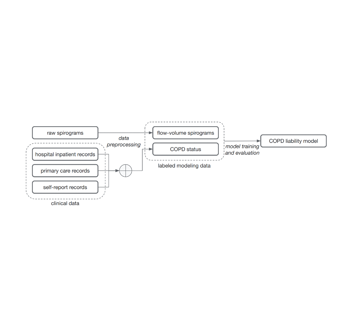
The common method of training models for this problem, supervised learning, requires samples to be associated with labels. Determining those labels can require the effort of very time-constrained experts. For this work, to show that we do not necessarily need medically graded labels, we decided to use a variety of widely available sources of medical record information to create those labels without medical expert review. These labels are less reliable and noisy for two reasons. First, there are gaps in the medical records of individuals because they use multiple health services. Second, COPD is often undiagnosed, meaning many with the disease will not be labeled as having it even if we compile the complete medical records. Nonetheless, we trained a model to predict these noisy labels from the spirogram curves and treat the model predictions as a quantitative COPD liability or risk score.
 |
| Noisy COPD status labels were derived using various medical record sources (clinical data). A COPD liability model is then trained to predict COPD status from raw flow-volume spirograms. |
Predicting COPD outcomes
We then investigated whether the risk scores produced by our model could better predict a variety of binary COPD outcomes (for example, an individual’s COPD status, whether they were hospitalized for COPD or died from it). For comparison, we benchmarked the model relative to expert-defined measurements required to diagnose COPD, specifically FEV1/FVC, which compares specific points on the spirogram curve with a simple mathematical ratio. We observed an improvement in the ability to predict these outcomes as seen in the precision-recall curves below.
 |
| Precision-recall curves for COPD status and outcomes for our ML model (green) compared to traditional measures. Confidence intervals are shown by lighter shading. |
We also observed that separating populations by their COPD model score was predictive of all-cause mortality. This plot suggests that individuals with higher COPD risk are more likely to die earlier from any causes and the risk probably has implications beyond just COPD.
 |
| Survival analysis of a cohort of UK Biobank individuals stratified by their COPD model’s predicted risk quartile. The decrease of the curve indicates individuals in the cohort dying over time. For example, p100 represents the 25% of the cohort with greatest predicted risk, while p50 represents the 2nd quartile. |
Identifying the genetic links with COPD
Since the goal of large scale biobanks is to bring together large amounts of both phenotype and genetic data, we also performed a test called a genome-wide association study (GWAS) to identify the genetic links with COPD and genetic predisposition. A GWAS measures the strength of the statistical association between a given genetic variant — a change in a specific position of DNA — and the observations (e.g., COPD) across a cohort of cases and controls. Genetic associations discovered in this manner can inform drug development that modifies the activity or products of a gene, as well as expand our understanding of the biology for a disease.
We showed with our ML-phenotyping method that not only do we rediscover almost all known COPD variants found by manual phenotyping, but we also find many novel genetic variants significantly associated with COPD. In addition, we see good agreement on the effect sizes for the variants discovered by both our ML approach and the manual one (R2=0.93), which provides strong evidence for validity of the newly found variants.
 |
| Left: A plot comparing the statistical power of genetic discovery using the labels for our ML model (y-axis) with the statistical power of the manual labels from a traditional study (x-axis). A value above the y = x line indicates greater statistical power in our method. Green points indicate significant findings in our method that are not found using the traditional approach. Orange points are significant in the traditional approach but not ours. Blue points are significant in both. Right: Estimates of the association effect between our method (y-axis) and traditional method (x-axis). Note that the relative values between studies are comparable but the absolute numbers are not. |
Finally, our collaborators at Harvard Medical School and Brigham and Women’s Hospital further examined the plausibility of these findings by providing insights into the possible biological role of the novel variants in development and progression of COPD (you can see more discussion on these insights in the paper).
Conclusion
We demonstrated that our earlier methods for phenotyping with ML can be expanded to a wide range of diseases and can provide novel and valuable insights. We made two key observations by using this to predict COPD from spirograms and discovering new genetic insights. First, domain knowledge was not necessary to make predictions from raw medical data. Interestingly, we showed the raw medical data is probably underutilized and the ML model can find patterns in it that are not captured by expert-defined measurements. Second, we do not need medically graded labels; instead, noisy labels defined from widely available medical records can be used to generate clinically predictive and genetically informative risk scores. We hope that this work will broadly expand the ability of the field to use noisy labels and will improve our collective understanding of lung function and disease.
Acknowledgments
This work is the combined output of multiple contributors and institutions. We thank all contributors: Justin Cosentino, Babak Alipanahi, Zachary R. McCaw, Cory Y. McLean, Farhad Hormozdiari (Google), Davin Hill (Northeastern University), Tae-Hwi Schwantes-An and Dongbing Lai (Indiana University), Brian D. Hobbs and Michael H. Cho (Brigham and Women’s Hospital, and Harvard Medical School). We also thank Ted Yun and Nick Furlotte for reviewing the manuscript, Greg Corrado and Shravya Shetty for support, and Howard Yang, Kavita Kulkarni, and Tammi Huynh for helping with publication logistics.

Get ready for Google I/O

Posted by Timothy Jordan, Director, Developer Relations & Open Source

I/O is just a few days away and we couldn’t be more excited to share the latest updates across Google’s developer products, solutions, and technologies. From keynotes to technical sessions and hands-on workshops, these announcements aim to help you build smarter and ship faster.
Here are some helpful tips to maximize your experience online.
Start building your personal I/O agenda
Starting now, you can save the Google and developer keynotes to your calendar and explore the program to preview content. Here are just a few noteworthy examples of what you’ll find this year:
What’s new in Android
Get the latest news in Android development: Android 14, form factors, Jetpack + Compose libraries, Android Studio, and performance.
What’s new in Web
Explore new features and APIs that became stable across browsers on the Web Platform this year.
What’s new in Generative AI
Discover a new suite of tools that make it easy for developers to leverage and build on top of Google’s large language models.
What’s new in Google Cloud
Learn how Google Cloud and generative AI will help you develop faster and more efficiently.
For the best experience, create or connect a developer profile and start saving content to My I/O to build your personal agenda. With over 200 sessions and other learning material, there’s a lot to cover, so we hope this will help you get organized.
This year we’ve introduced development focus filters to help you navigate content faster across mobile, web, AI, and cloud technologies. You can also peruse content by topic, type, or experience level so you can find what you’re interested in, faster.
Connect with the community
After the keynotes, you can talk to Google experts and other developers online in I/O Adventure chat. Here you can ask questions about new releases and learn best practices from the global developer community.
If you’re craving community now, visit the Community page to meet people with similar interests in your area or find a watch party to attend.
We hope these updates are useful, and we can’t wait to connect online in May!
Improve multi-hop reasoning in LLMs by learning from rich human feedback
Recent large language models (LLMs) have enabled tremendous progress in natural language understanding. However, they are prone to generating confident but nonsensical explanations, which poses a significant obstacle to establishing trust with users. In this post, we show how to incorporate human feedback on the incorrect reasoning chains for multi-hop reasoning to improve performance on these tasks. Instead of collecting the reasoning chains from scratch by asking humans, we instead learn from rich human feedback on model-generated reasoning chains using the prompting abilities of the LLMs. We collect two such datasets of human feedback in the form of (correction, explanation, error type) for StrategyQA and Sports Understanding datasets, and evaluate several common algorithms to learn from such feedback. Our proposed methods perform competitively to chain-of-thought prompting using the base Flan-T5, and ours is better at judging the correctness of its own answer.
Solution overview
With the onset of large language models, the field has seen tremendous progress on various natural language processing (NLP) benchmarks. Among them, the progress has been striking on relatively simpler tasks such as short context or factual question answering, compared to harder tasks that require reasoning such as multi-hop question answering. The performance of certain tasks using LLMs may be similar to random guessing at smaller scales, but improves significantly at larger scales. Despite this, the prompting abilities of LLMs have the potential to provide some relevant facts required to answer the question.
However, those models may not reliably generate correct reasoning chains or explanations. Those confident but nonsensical explanations are even more prevalent when LLMs are trained using Reinforcement Learning from Human Feedback (RLHF), where reward hacking may occur.
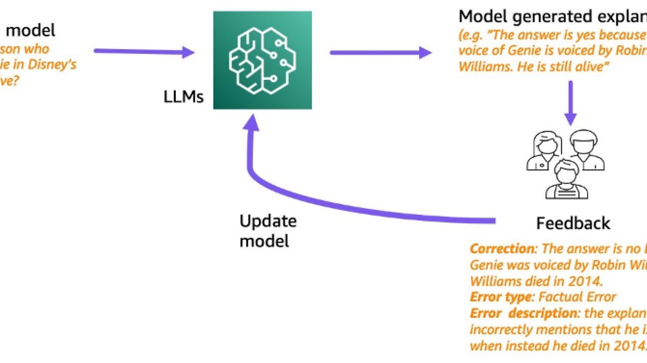
Motivated by this, we try to address the following research question: can we improve reasoning of LLMs by learning from human feedback on model-generated reasoning chains? The following figure provides an overview of our approach: we first prompt the model to generate reasoning chains for multi-hop questions, then collect diverse human feedback on these chains for diagnosis and propose training algorithms to learn from the collected data.

We collect diverse human feedback on two multi-hop reasoning datasets, StrategyQA and Sports Understanding from BigBench. For each question and model-generated reasoning chain, we collect the correct reasoning chain, the type of error in the model-generated reasoning chain, and a description (in natural language) of why that error is presented in the provided reasoning chain. The final dataset contains feedback for 1,565 samples from StrategyQA and 796 examples for Sports Understanding.
We propose multiple training algorithms to learn from the collected feedback. First, we propose a variant of self-consistency in chain-of-thought prompting by considering a weighted variant of it that can be learned from the feedback. Second, we propose iterative refinement, where we iteratively refine the model-generated reasoning chain until it’s correct. We demonstrate empirically on the two datasets that fine-tuning an LLM, namely Flan-T5 using the proposed algorithms, performs comparably to the in-context learning baseline. More importantly, we show that the fine-tuned model is better at judging if its own answer is correct compared to the base Flan-T5 model.
Data collection
In this section, we describe the details of the feedback we collected and the annotation protocol followed during data collection. We collected feedback for model generations based on two reasoning-based datasets: StrategyQA and Sports Understanding from BigBench. We used GPT-J to generate the answer for StrategyQA and Flan-T5 to generate the answer for the Sports Understanding dataset. In each case, the model was prompted with k in-context examples containing question, answer, and explanation, followed by the test question.
The following figure shows the interface we used. Annotators are given the question, the model-generated answer, and the explanation split into steps.

For each question, we collected the following feedback:
- Subquestions – The annotators decompose the original question into simpler subquestions required to answer the original question. This task was added after a pilot where we found that adding this task helps prepare the annotators and improve the quality of the rest of the tasks.
- Correction – Annotators are provided with a free-form text box pre-filled with the model-generated answer and explanation, and asked to edit it to obtain the correct answer and explanation.
- Error type – Among the most common types of error we found in the model generations (Factual Error, Missing Facts, Irrelevant Facts, and Logical Inconsistency), annotators were asked to pick one or more of the error types that apply to the given answer and explanation.
- Error description – The annotators were instructed to not only classify the errors but also give a comprehensive justification for their categorization, including pinpointing the exact step where the mistake occurred and how it applies to the answer and explanation provided.
We used Amazon SageMaker Ground Truth Plus in our data collection. The data collection took place over multiple rounds. We first conducted two small pilots of 30 examples and 200 examples, respectively, after which the annotator team was given detailed feedback on the annotation. We then conducted the data collection over two batches for StrategyQA, and over one batch for Sports Understanding, giving periodic feedback throughout—a total of 10 annotators worked on the task over a period of close to 1 month.
We gathered feedback on a total of 1,565 examples for StrategyQA and 796 examples for Sports Understanding. The following table illustrates the percentage of examples that were error-free in the model generation and the proportion of examples that contained a specific error type. It’s worth noting that some examples may have more than one error type.
| Error Type | StrategyQA | Sports Understanding |
| None | 17.6% | 31.28% |
| Factual Error | 27.6% | 38.1% |
| Missing Facts | 50.4% | 46.1% |
| Irrelevant Facts | 14.6% | 3.9% |
| Logical Inconsistency | 11.2% | 5.2% |
Learning algorithms
For each question q, and model-generated answer and explanation m, we collected the following feedback: correct answer and explanation c, type of error present in m (denoted by t), and error description d, as described in the previous section.
We used the following methods:
- Multitask learning – A simple baseline to learn from the diverse feedback available is to treat each of them as a separate task. More concretely, we fine-tune Flan-T5 (text to text) with the objective maximize p(c|q) + p(t|q, m) + p(d|q, m). For each term in the objective, we use a separate instruction appropriate for the task (for example, “Predict error in the given answer”). We also convert the categorical variable t into a natural language sentence. During inference, we use the instruction for the term p(c|q) (“Predict the correct answer for the given question”) to generate the answer for the test question.
- Weighted self-consistency – Motivated by the success of self-consistency in chain-of-thought prompting, we propose a weighted variant of it. Instead of treating each sampled explanation from the model as correct and considering the aggregate vote, we instead first consider whether the explanation is correct and then aggregate accordingly. We first fine-tune Flan-T5 with the same objective as in multitask learning. During inference, given a test question q, we sample multiple possible answers with the instruction for p(c|q)): a1, a2, .., an. For each sampled answer ai, we use the instruction for the term p(t|q, m) (“Predict error in the given answer”) to identify if it contains error ti = argmax p(t|q, a_i). Each answer ai is assigned a weight of 1 if it’s correct, otherwise it’s assigned a weight smaller than 1 (tunable hyperparameter). The final answer is obtained by considering a weighted vote over all the answers a1 to an.
- Iterative refinement – In the previous proposed methods, the model directly generates the correct answer c conditioned on the question q. Here we propose to refine the model-generated answer m to obtain the correct answer for a given question. More specifically, we first fine-tune Flan-T5 (text to text with the objective) with maximize p(t; c|q, m), where ; denotes the concatenation (error type t followed by the correct answer c). One way to view this objective is that the model is first trained to identify the error in given generation m, and then to remove that error to obtain the correct answer c. During inference, we can use the model iteratively until it generates the correct answer—given a test question q, we first obtain the initial model generation m (using pre-trained Flan-T5). We then iteratively generate the error type ti and potential correct answer ci until ti = no error (in practice, we set a maximum number of iterations to a hyperparameter), in which case the final correct answer will be ci-1 (obtained from p(ti ; ci | q, ci-1)).
Results
For both datasets, we compare all the proposed learning algorithms with the in-context learning baseline. All models are evaluated on the dev set of StrategyQA and Sports Understanding. The following table shows the results.
| Method | StrategyQA | Sports Understanding |
| Flan-T5 4-shot Chain-of-Thought In-Context Learning | 67.39 ± 2.6% | 58.5% |
| Multitask Learning | 66.22 ± 0.7% | 54.3 ± 2.1% |
| Weighted Self Consistency | 61.13 ± 1.5% | 51.3 ± 1.9% |
| Iterative Refinement | 61.85 ± 3.3% | 57.0 ± 2.5% |
As observed, some methods perform comparable to the in-context learning baseline (multitask for StrategyQA, and iterative refinement for Sports Understanding), which demonstrates the potential of gathering ongoing feedback from humans on model outputs and using that to improve language models. This is different from recent work such as RLHF, where the feedback is limited to categorical and usually binary.
As shown in the following table, we investigate how models adapted with human feedback on reasoning mistakes can help improve the calibration or the awareness of confidently wrong explanations. This is evaluated by prompting the model to predict if its generation contains any errors.
| Method | Error Correction | StrategyQA |
| Flan-T5 4-shot Chain-of-Thought In-Context Learning | No | 30.17% |
| Multitask Finetuned Model | Yes | 73.98% |
In more detail, we prompt the language model with its own generated answer and reasoning chain (for which we collected feedback), and then prompt it again to predict the error in the generation. We use the appropriate instruction for the task (“Identify error in the answer”). The model is scored correctly if it predicts “no error” or “correct” in the generation if the annotators labeled the example as having no error, or if it predicts any of the error types in the generation (along with “incorrect” or “wrong”) when the annotators labeled it as having an error. Note that we don’t evaluate the model’s ability to correctly identify the error type, but rather if an error is present. The evaluation is done on a set of 173 additional examples from the StrategyQA dev set that were collected, which aren’t seen during fine-tuning. Four examples out of these are reserved for prompting the language model (first row in the preceding table).
Note that we do not show the 0-shot baseline result because the model is unable to generate useful responses. We observe that using human feedback for error correction on reasoning chains can improve the model’s prediction of whether it makes errors or not, which can improve the awareness or calibration of the wrong explanations.
Conclusion
In this post, we showed how to curate human feedback datasets with fine-grained error corrections, which is an alternative way to improve the reasoning abilities of LLMs. Experimental results corroborate that human feedback on reasoning errors can improve performance and calibration on challenging multi-hop questions.
If you’re looking for human feedback to improve your large language models, visit Amazon SageMaker Data Labeling and the Ground Truth Plus console.
About the Authors
 Erran Li is the applied science manager at humain-in-the-loop services, AWS AI, Amazon. His research interests are 3D deep learning, and vision and language representation learning. Previously he was a senior scientist at Alexa AI, the head of machine learning at Scale AI and the chief scientist at Pony.ai. Before that, he was with the perception team at Uber ATG and the machine learning platform team at Uber working on machine learning for autonomous driving, machine learning systems and strategic initiatives of AI. He started his career at Bell Labs and was adjunct professor at Columbia University. He co-taught tutorials at ICML’17 and ICCV’19, and co-organized several workshops at NeurIPS, ICML, CVPR, ICCV on machine learning for autonomous driving, 3D vision and robotics, machine learning systems and adversarial machine learning. He has a PhD in computer science at Cornell University. He is an ACM Fellow and IEEE Fellow.
 Nitish Joshi was an applied science intern at AWS AI, Amazon. He is a PhD student in computer science at New York University’s Courant Institute of Mathematical Sciences advised by Prof. He He. He works on Machine Learning and Natural Language Processing, and he was affiliated with the Machine Learning for Language (ML2) research group. He was broadly interested in robust language understanding: both in building models which are robust to distribution shifts (e.g. through human-in-the-loop data augmentation) and also in designing better ways to evaluate/measure the robustness of models. He has also been curious about the recent developments in in-context learning and understanding how it works.
 Kumar Chellapilla is a General Manager and Director at Amazon Web Services and leads the development of ML/AI Services such as human-in-loop systems, AI DevOps, Geospatial ML, and ADAS/Autonomous Vehicle development. Prior to AWS, Kumar was a Director of Engineering at Uber ATG and Lyft Level 5 and led teams using machine learning to develop self-driving capabilities such as perception and mapping. He also worked on applying machine learning techniques to improve search, recommendations, and advertising products at LinkedIn, Twitter, Bing, and Microsoft Research.
How to extend the functionality of AWS Trainium with custom operators
Deep learning (DL) is a fast-evolving field, and practitioners are constantly innovating DL models and inventing ways to speed them up. Custom operators are one of the mechanisms developers use to push the boundaries of DL innovation by extending the functionality of existing machine learning (ML) frameworks such as PyTorch. In general, an operator describes the mathematical function of a layer in a deep learning model. A custom operator allows developers to build their own mathematical functions for a layer in the deep learning model.
AWS Trainium and AWS Inferentia2, which are purpose built for DL training and inference, extend their functionality and performance by supporting custom operators (or CustomOps, for short). AWS Neuron, the SDK that supports these accelerators, uses the standard PyTorch interface for CustomOps. Developers can easily get started with their existing code when using Trainium-based Amazon EC2 Trn1 instances or Inferentia2-based Amazon EC2 Inf2 instances. In this post, we cover the benefits of CustomOps, their efficient implementation on Trainium, and examples to get you started with CustomOps on Trainium-powered Trn1 instances.
To follow along, familiarity with core AWS services such as Amazon Elastic Compute Cloud (Amazon EC2) is implied, and basic familiarity with deep learning, PyTorch, and C++ would be helpful.
Custom operators in PyTorch and their benefits
CustomOps for PyTorch originated in version 1.10, called PyTorch C++ Frontend, and provided an easy-to-use mechanism to register CustomOps written in C++. The following are some of the benefits that CustomOps provide:
- Performance optimization – CustomOps can be optimized for specific use cases, leading to faster model runs and improved performance.
- Improved model expressiveness – With CustomOps, you can express complex computations that aren’t easily expressible using the built-in operators provided by PyTorch.
- Increased modularity – You can use CustomOps as building blocks to create more complex models by creating C++ libraries of reusable components. This makes the development process easier and more modular, and facilitates rapid experimentation.
- Increased flexibility – CustomOps enables operations beyond the built-in operators—that is, they provide a flexible way to define complex operations that aren’t implemented using the standard ones.
Trainium support for custom operators
Trainium (and AWS Inferentia2) supports CustomOps in software through the Neuron SDK and accelerates them in hardware using the GPSIMD engine (General Purpose Single Instruction Multiple Data engine). Let’s look at how these enable efficient CustomOps implementation and provide increased flexibility and performance when developing and innovating DL models.
Neuron SDK
The Neuron SDK helps developers train models on Trainium and deploy models on the AWS Inferentia accelerators. It integrates natively with frameworks, such as PyTorch and TensorFlow, so you can continue using your existing workflows and application code to train models on Trn1 instances.
The Neuron SDK uses the standard PyTorch interface for CustomOps. Developers can use the standard programming interface in PyTorch to write CustomOps in C++ and extend Neuron’s official operator support. Neuron then compiles these CustomOps to run efficiently on the GPSIMD engine, which is described in more detail in the following section. This makes it easy to implement new experimental CustomOps and accelerate them on purpose-built hardware, without any intimate knowledge of this underlying hardware.
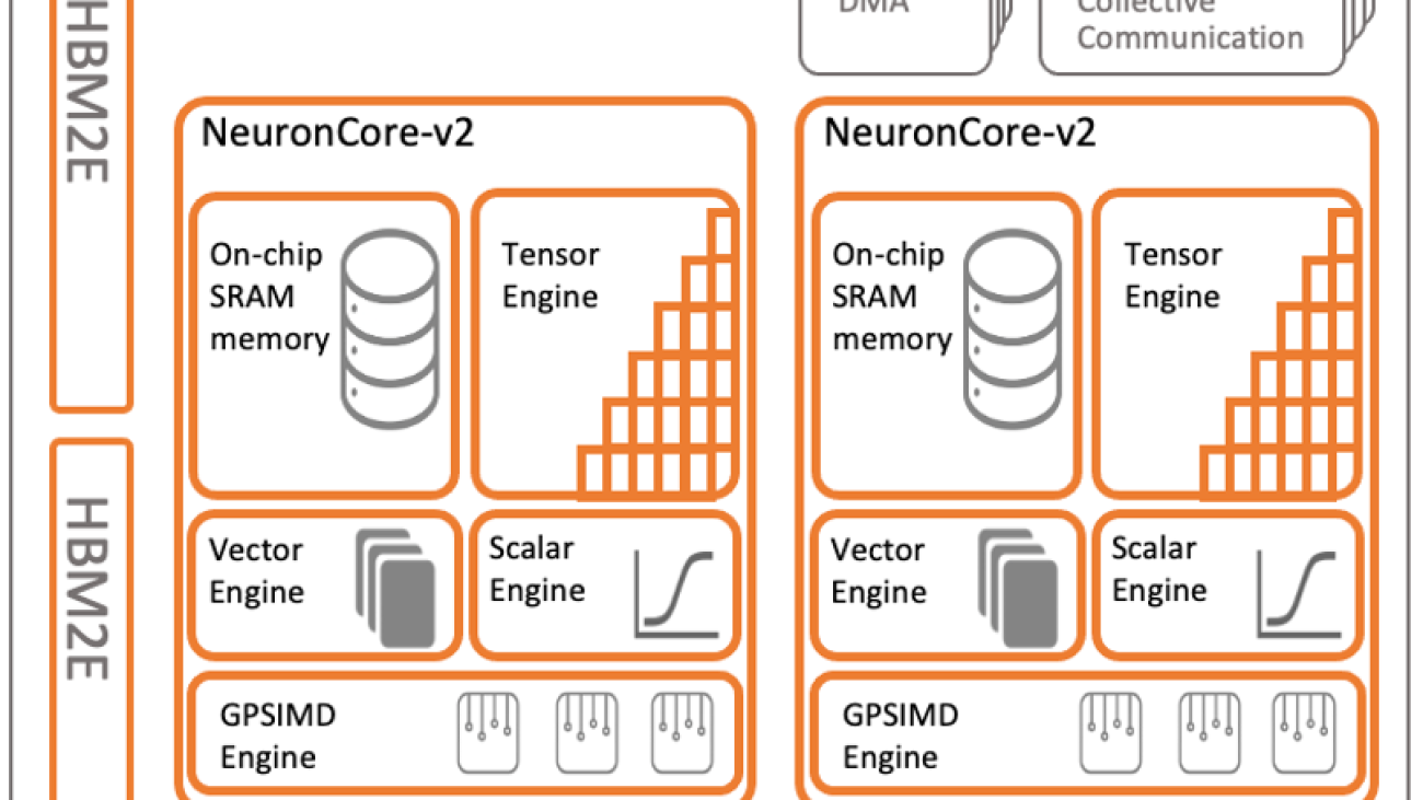
General Purpose Single Instruction Multiple Data engine
At the core of Trainium optimizations resides the NeuronCore architecture, a fully independent, heterogeneous compute-unit with four main engines: tensor, vector, scalar, and the GPSIMD engine. The scalar and vector engines are highly parallelized and optimized for floating-point operations. The tensor engine is based on a power-optimized, systolic-array supporting mixed precision computation.

The GPSIMD engine is a general-purpose Single Instruction Multiple Data (SIMD) engine designed for running and accelerating CustomOps. This engine consists of eight fully programmable 512-bit wide general-purpose processors, which can run straight-line C-code and have direct inline access to the other NeuronCore-v2 engines, as well as the embedded SRAM and HBM memories. Together, these capabilities help run CustomOps efficiently on Trainium.
Take for example operators such as TopK, LayerNorm, or ZeroCompression, which read data from memory and only use it for a minimal number of ALU calculations. Regular CPU systems are completely memory bound for these calculations, and performance is limited by the time required to move the data into the CPU. In Trainium, the GP-SIMD engines are tightly coupled with the on-chip caches using a high bandwidth streaming interface, which can sustain 2 TB/sec of memory bandwidth. Therefore, CustomOps like these can be run really fast on Trainium.
Neuron SDK custom operators in practice
For this post, we assume a DLAMI (refer to instructions for either Ubuntu or Amazon Linux) is being used to instantiate an EC2 Trn1 instance (either 2x.large or 32x.large). Note all necessary software, drivers, and tools have already been installed on the DLAMIs, and only the activation of the Python environment is needed to start working with the tutorial. We reference the CustomOps functionality available in Neuron as “Neuron CustomOps.”
Similar to the process of PyTorch integration with C++ code, Neuron CustomOps requires a C++ implementation of an operator via a NeuronCore-ported subset of the Torch C++ API . The C++ implementation of the operator is called the kernel function, and the port of the C++ API contains everything required for CustomOps development and model integration, specifically tensor and scalar classes in c10 (a namespace used for low-level C++ code across different PyTorch libraries), and a subset of ATen operators (or Automatic Tensor, the C++ library that provides the core tensor operations used in PyTorch).
The torch.h header needs to be included when defining the kernel for you to have access to a NeuronCore-ported subset of the Pytorch C++ API:
Neuron CustomOps also require a shape function. The shape function has the same function signature as the kernel function, but doesn’t perform any computations. It only defines the shape of the output tensor but not the actual values.
Neuron CustomOps are grouped into libraries, and macros are used to register them with the NEURON_LIBRARY scope from within the shape function. The function will be run on the host at compilation time and will require the register.h header from the torchneuron library:
Finally, the custom library is built by calling the load API. If supplying the build_directory parameter, the library file will be stored in the indicated directory:

To use the CustomOp from a PyTorch model, simply load the library by calling the load_library API and call the Neuron CustomOp in the same manner that CustomOps are called in PyTorch via the torch.ops namespace. The format is usually torch.ops.<library_name>.<operator_name>. See the following code:
Note that the custom_op.load API builds the C++ library, whereas the custom_op.load_library API loads an already-built library file.
Example: Neuron CustomOps in MLP training
To get started, perform the following steps:
- Create and launch your EC2 Trn1 instance. Be sure that you use a DLAMI image (either Ubuntu or Amazon Linux, pre-installed with all necessary Neuron software) and that you have specified a root volume size of 512 GB.
- After your instance is up and running, SSH to your instance.
- Install PyTorch Neuron (torch-neuronx) on your running Trn1 instance. For instructions, refer to Neuron Custom C++ Operators in MLP Training.
- Download the sample code from the GitHub repository.
Now that your environment is set up, continue through this post as we describe the implementation of a typical C++ CustomOp in Neuron in the form of Relu forward and backward functions to be used on a simple multilayer perceptron (MLP) model. The steps are described in the AWS Neuron Documentation.
The example code from the repository shows two folders:
- ./customop_mlp/PyTorch – Contains the Relu code that will be compiled for a CPU
- ./customop_mlp/neuron – Contains the Relu code that will be compiled for Trainium
Develop a Neuron CustomOp: The kernel function
The host or dev environment for the development of the kernel function (the Neuron CustomOp) can run PyTorch 1.13 and a C++17 compatible compiler in a Linux environment. This is the same as developing any C++ function for PyTorch, and the only libraries that need to be present in the development environment are those for PyTorch and C++. In the following example, we create a relu.cpp file with the custom Relu forward and backward functions:
When developing a Neuron CustomOp for Neuron, make sure you take into account the currently supported features and APIs. For more information, refer to Custom Operators API Reference Guide [Experimental].
Build and register the Neuron CustomOp: The shape function
The build for the Neuron CustomOp and runtime environment is the Trn1 instance where the training will take place, and the Neuron CustomOp will be compiled and registered as a neuronx-cc library and interpreted by the Neuron runtime to run on the highly optimized GP-SIMD engine.
To build and register the Neuron CustomOp, we need to create a shape function (shape.cpp) that will define the input and output tensors and register the operators: the relu_fwd_shape and relu_bwd_shape functions. See the following code:
The relu_fwd_shape and relu_bwd_shape functions define the shape of the output tensor (to be the same size as the input tensor). Then we register the functions in the NEURON_LIBRARY scope.
In the ./customop_ml/neuron repository example, we have a build.py script to run the build and registration of the CustomOp, by simply calling the load function from the torch_neuronx.xla_impl package:
In the build_directory, we should find the librelu.so library ready to be loaded and used in training our model.
Build the MLP model with the Neuron CustomOp
In this section, we go through the steps to build the MLP model with the Neuron CustomOp.
Define the Relu class
For a detailed explanation of how to train an MLP model, refer to Multi-Layer Perceptron Training Tutorial.
After we build the CustomOp, we create a Python package called my_ops.py, where we define a Relu PyTorch class, inheriting from the torch autograd function. The autograd function implements automatic differentiation, so that it can be used in a training loop.
First we load the librelu.so library, then we define the new class with the forward and backward functions defined with static method decorators. In this way, the methods can be called directly when we define the model. See the following code:
Examine the MLP model
Now we’re ready to write our multilayer perceptron model with our Neuron CustomOp by importing the my_ops package where we have defined the Relu class:
Run the training script
Now we can train our model by using the train.py provided script:
By sending the model to the xla device, the model and Relu custom operator are compiled to be run by the Neuron runtime using the optimized Trainium hardware.
In this example, we showed how to create a custom Relu operator that takes advantage of the hardware engine (GP-SIMD) available on the Trainium ML accelerator chip. The result is a trained PyTorch model that can now be deployed for inferencing.
Conclusion
Modern state-of-the-art model architectures require an increasing number of resources from engineering staff (data scientists, ML engineers, MLOps engineers, and others) to actual infrastructure including storage, compute, memory, and accelerators. These requirements increase the cost and complexity of developing and deploying deep learning models. Trainium accelerators deliver a high-performance, low-cost solution for DL training in the cloud. The use of Trainium is facilitated by the Neuron SDK, which includes a deep learning compiler, runtime, and tools that are natively integrated into popular frameworks such as PyTorch and TensorFlow. (Note that at the time of writing, the Neuron SDK 2.9 only supports PyTorch for the development of custom operators.)
As demonstrated in this post, Trainium not only provides the means to train your models performantly and efficiently, but also offers the ability to customize your operators to add flexibility and expressiveness to both training and experimentation.
For more information, refer to the GitHub repo.
About the Authors
 Lorea Arrizabalaga is a Solutions Architect aligned to the UK Public Sector, where she helps customers design ML solutions with Amazon SageMaker. She is also part of the Technical Field Community dedicated to hardware acceleration and helps with testing and benchmarking AWS Inferentia and AWS Trainium workloads.
 Shruti Koparkar is a Senior Product Marketing Manager at AWS. She helps customers explore, evaluate, and adopt Amazon EC2 accelerated computing infrastructure for their machine learning needs.

What Is Agent Assist?
“Please hold” may be the two words that customers hate most — and that contact center agents take pains to avoid saying.
Providing fast, accurate, helpful responses based on contextually relevant information is key to effective customer service. It’s even better if answers are personalized and take into account how a customer might be feeling.
All of this is made easier and quicker for human agents by what the industry calls agent assists.
Agent assist technology uses AI and machine learning to provide facts and make real-time suggestions that help human agents across telecom, retail and other industries conduct conversations with customers.
It can integrate with contact centers’ existing applications, provide faster onboarding for agents, improve the accuracy and efficiency of their responses, and increase customer satisfaction and loyalty.
How Agent Assist Technology Works
Agent assist technology gives human agents AI-powered information and real-time recommendations that can enhance their customer conversations.
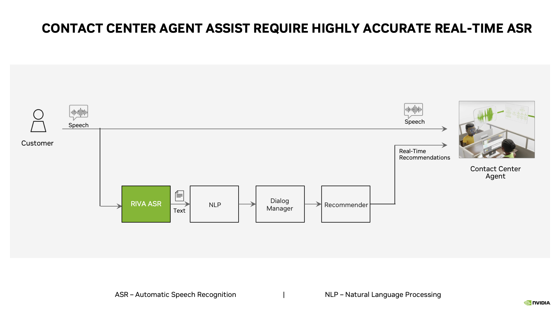
Taking conversations as input, agent assist technology outputs accurate, timely suggestions on how to best respond to queries — using a combination of automatic speech recognition (ASR), natural language processing (NLP), machine learning and data analytics.
While a customer speaks to a human agent, ASR tools — like the NVIDIA Riva software development kit — transcribe speech into text, in real time. The text can then be run through NLP, AI and machine learning models that offer recommendations to the human agent by analyzing different aspects of the conversation.
First, AI models can evaluate the context of the conversation, identify topics and bring up relevant information for the human agent — like the customer’s account data , a record of their previous inquiries, documents with recommended products and additional information to help resolve issues.
Say a customer is looking to switch to a new phone plan. The agent assist could, for example, immediately display a chart on the human agent’s screen comparing the company’s offerings, which can be used as a reference throughout the conversation.
Another AI model can perform sentiment analysis based on the words a customer is using.
For example, if a customer says, “I’m extremely frustrated with my cellular reception,” the agent assist would advise the human agent to approach the customer differently from a situation where the customer says, “I am happy with my phone plan but am looking for something less expensive.”
It can even present a human agent with verbiage to consider using when soothing, encouraging, informing or otherwise guiding a customer toward conflict resolution.
And, at a conversation’s conclusion, agent assist technology can provide personalized, best next steps for the human agent to give the customer. It can also offer the human agent a summary of the interaction overall, along with feedback to inform future conversations and employee training.
All such ASR, NLP and AI-powered capabilities come together in agent assist technology, which is becoming increasingly integral to businesses across industries.
How Agent Assist Technology Helps Businesses, Customers
By tapping into agent assist technology, businesses can improve productivity, employee retention and customer satisfaction, among other benefits.
For one, agent assist technology reduces contact center call times. Through NLP and intelligent routing algorithms, it can identify customer needs in real time, so human agents don’t need to hunt for basic customer information or search databases for answers.
Leading telecom provider T-Mobile — which offers award-winning service across its Customer Experience Centers — uses agent assist technology to help tackle millions of daily customer care calls. The NVIDIA NeMo framework helped the company achieve 10% higher accuracy for its ASR-generated transcripts across noisy environments, and Riva reduced latency for its agent assist by 10x. (Dive deeper into speech AI by watching T-Mobile’s on-demand NVIDIA GTC session.)
Agent assist technology also speeds up the onboarding process for human agents, helping them quickly become familiar with the products and services offered by their organization. In addition, it empowers contact center employees to provide high levels of service while maintaining low levels of stress — which means higher employee retention for enterprises.
Quicker, more accurate conflict resolution enabled by agent assist also leads to more positive contact center experiences, happier customers and increased loyalty for businesses.
Use Cases Across Industries
Agent assist technology can be used across industries, including:
- Telecom — Agent assist can provide automated troubleshooting, technical tips and other helpful information for agents to relay to customers.
- Retail — Agent assist can suggest products, features, pricing, inventory information and more in real time, as well as translate languages according to customer preferences.
- Financial services — Agent assist can help detect fraud attempts by providing real-time alerts, so that human agents are aware of any suspicious activity throughout an inquiry.
Minerva CQ, a member of the NVIDIA Inception program for cutting-edge startups, provides agent assist technology that brings together real-time, adaptive workflows with behavioral cues, dialogue suggestions and knowledge surfacing to drive faster, better outcomes. Its technology — based on Riva, NeMo and NVIDIA Triton Inference Server — focuses on helping human agents in the energy, healthcare and telecom sectors.
History and Future of Agent Assist
Predecessors of agent assist technology can be traced back to the 1950s, when computer-based systems first replaced manual call routing.
More recently came intelligent virtual assistants, which are usually automated systems or bots that don’t have a human working behind them.
Smart devices and mobile technology have led to a rise in the popularity of these intelligent virtual assistants, which can answer questions, set reminders, play music, control home devices and handle other simple tasks.
But complex tasks and inquiries — especially for enterprises with customer service at their core — can be solved most efficiently when human agents are augmented by AI-powered suggestions. This is where agent assist technology has stepped in.
The technology has much potential for further advancement, with challenges including:
- Developing methods for agent assists to adapt to changing customer expectations and preferences.
- Further ensuring data privacy and security through encryption and other methods to strip conversations of confidential or sensitive information before running them through agent assist AI models.
- Integrating agent assist with other emerging technologies like interactive digital avatars, which can see, hear, understand and communicate with end users to help customers while boosting their sentiment.
Learn more about NVIDIA speech AI technologies.
Additional resources:
- Webinar: How Telcos Transform Customer Experiences With Conversational AI.
- Webinar: Empower Telco Contact Center Agents With Multi-Language Speech-AI-Customized Agent Assists.
- On-Demand NVIDIA GTC Sessions: T-Mobile and AT&T
- Customer Story: T-Mobile

Welcome to the Family: GeForce NOW, Capcom Bring ‘Resident Evil’ Titles to the Cloud
Horror descends from the cloud this GFN Thursday with the arrival of publisher Capcom’s iconic Resident Evil series.
They’re part of nine new games expanding the GeForce NOW library of over 1,600 titles.
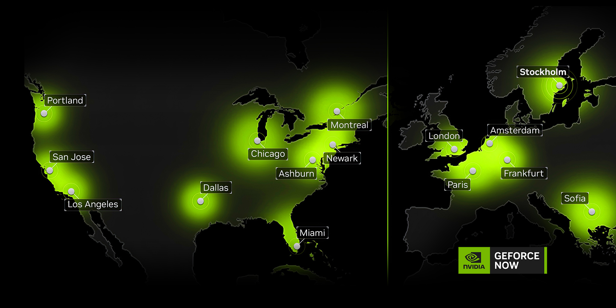
RTX 4080 SuperPODs are now live in Miami, Portland, Ore., and Stockholm. Follow along with the server rollout process, and make the Ultimate upgrade for unbeatable cloud gaming performance.
Survive in the Cloud

The Resident Evil series makes its debut on GeForce NOW with Resident Evil 2, Resident Evil 3 and Resident Evil 7 Biohazard.
Survive against hordes of flesh-eating zombies and other bio-organic creatures created by the sinister Umbrella Corporation in these celebrated — and terrifying — Resident Evil games. The survival horror games feature memorable casts of characters and gripping storylines to keep members glued to their seats.
With RTX ON and high dynamic range, Ultimate and Priority members will also experience the most realistic lighting and deepest shadows. Bonus points for streaming with the lights off for an even more immersive experience.
The Newness
The Resident Evil titles lead nine new games joining the GeForce NOW library:
- Shadows of Doubt (New release on Steam, April 24)
- Afterimage (New release on Steam, April 24)
- Roots of Pacha (New release on Steam, April 25)
- Bramble: The Mountain King (New release on Steam, April 27)
- The Swordsmen X: Survival (New release on Steam, April 27)
- Poker Club (Free on Epic Games Store, April 27)
- Resident Evil 2 (Steam)
- Resident Evil 3 (Steam)
- Resident Evil 7 Biohazard (Steam)
Best zombie fighting weapon. Go.
—
NVIDIA GeForce NOW (@NVIDIAGFN) April 26, 2023
And check out the question of the week. Let us know your answer in the comments below, or on the GeForce NOW Facebook and Twitter channels.