Posts in category: Tensorflow

Posted by Alan Kelly, Software Engineer

We are excited to announce that XNNPack’s Fully Connected and Convolution 2D operators now support dynamic range quantization. XNNPack is TensorFlow Lite’s CPU backend and CPUs deliver the widest reach for ML inference and remain the default target for TensorFlow Lite. Consequently, improving CPU inference performance is a top priority. We quadrupled inference performance in TensorFlow Lite’s XNNPack backend compared to the single precision baseline by adding support for dynamic range quantization to the Fully Connected and Convolution operators. This means that more AI powered features may be deployed to older and lower tier devices.

Previously, XNNPack offered users the choice between either full integer quantization, where the weights and activations are stored as signed 8-bit integers, or half-precision (fp16) or single-precision (fp32) floating-point inference. In this article we demonstrate the benefits of dynamic range quantization.

Dynamic Range Quantization

Dynamically quantized models are similar to fully-quantized models in that the weights for the Fully Connected and Convolution operators are quantized to 8-bit integers during model conversion. All other tensors are not quantized, they remain as float32 tensors. During model inference, the floating-point layer activations are converted to 8-bit integers before being passed to the Fully Connected and Convolution operators. The quantization parameters (the zero point and scale) for each row of the activation tensor are calculated dynamically based on the observed range of activations. This maximizes the accuracy of the quantization process as the activations make full use of the 8 quantized bits. In fully-quantized models, these parameters are fixed during model conversion, based on the range of the activation values observed using a representative dataset. The second difference between full quantization and dynamic range quantization is that the output of the Fully Connected and Convolution operators is in 32-bit floating-point format, as opposed to 8-bit integer for fully-quantized operators. With dynamic range quantization, we get most of the performance gains of full quantization, yet with higher overall accuracy.

Traditionally the inference of such models was done using TensorFlow Lite’s native operators. Now dynamically quantized models can benefit from XNNPack’s highly-optimized per-architecture implementations of the Fully Connected and Convolution2D operators. These operators are optimized for all architectures supported by XNNPack (ARM, ARM64, x86 SSE/AVX/AVX512 and WebAssembly), including the latest ArmV9 processors such as the Pixel 8’s Tensor G3 CPU or the One Plus 11’s SnapDragon 8 Gen 2 CPU.

How can you use it?

Two steps are required to use dynamic range quantization. You must first convert your model from TensorFlow with support for dynamic range quantization. Existing models already converted using dynamic range quantization do not need to be reconverted. Dynamic range quantization can be enabled during model conversion by enabling the
converter.optimizations = [tf.lite.Optimize.DEFAULT] converter flag. Unlike full integer quantization, no representative dataset is required and unsupported operators do not prevent conversion from succeeding. Dynamic range quantization is therefore far more accessible to non-expert users than full integer quantization.

From TensorFlow 2.17, dynamically quantized XNNPack inference will be enabled by default in prebuilt binaries. If you want to use it sooner, the nightly TensorFlow builds may be used.

Mixed Precision Inference

In our previous article we presented the impressive performance gains from using half precision inference. Half-precision and dynamic range quantization may now be combined within XNNPack to get the best possible on-device CPU inference performance on devices which have hardware fp16 support (most phones on sale today do). The Fully Connected and Convolution 2D operators can output fp16 data instead of fp32. The Pixel 3, released in 2018, was the first Pixel model with fp16 support. fp16 uses half as many bits to store a floating-point value compared to fp32, meaning that the relative accuracy of each value is reduced due to the significantly shorter mantissa (10 vs 23 bits). Not all models support fp16 inference, but if a model supports it, the computational cost of vectorized floating-point operators can be reduced by half as the CPU can process twice as much data per instruction. Dynamically quantized models with compute-intensive floating point operators, such as Batch Matrix Multiply and Softmax, can benefit from fp16 inference as well.

Performance Improvements

Below, we present benchmarks on four public models covering common computer vision tasks:

1. EfficientNetV2 – image classification and feature extraction
2. Inception-v3 – image classification
3. Deeplab-v3 – semantic segmentation
4. Stable Diffusion – image generation (diffusion model)

Each model was converted three times where possible: full float, full 8 bit signed integer quantization and dynamic range quantization. Stable Diffusion’s diffusion model could not be converted using full integer quantization due to unsupported operators. The speed-up versus the original float32 model using TFLite’s kernels is shown below.

• FP32 refers to the baseline float32 model.
• QS8 refers to full signed 8 bit integer quantization using XNNPack.
• QD8-F32 refers to dynamically quantized 8 bit integers with fp32 activations using XNNPack.
• QD8-F16 refers to dynamically quantized 8 bit integers with fp16 activations using XNNPack.

The speed-up versus TFLite’s dynamically quantized Fully Connected and Convolution operators are shown below. By simply using the latest version of TensorFlow Lite, you can benefit from these speed-ups.

We can clearly see that dynamic range quantization is competitive with, and in some cases can exceed, the performance of full integer quantization. Stable Diffusion’s diffusion model runs up to 6.2 times faster than the original float32 model! This is a game changer for on-device performance.

We would expect that full integer quantization would be faster than dynamic range quantization as all operations are calculated using integer arithmetic. Furthermore, dynamic range quantization has the additional overhead of converting the floating point activations to quantized 8 bit integers. Surprisingly, in two of the three models tested, this is not true. Profiling the models using TFLite’s profiler solves the mystery. These models are slower due to a combination of quantization artifacts — quantized arithmetic is more efficient when the ratio of the input and output scales fall within a certain range and missing op support in XNNPack. These quantization parameters are determined during model conversion based on a provided representative dataset. Since the ratio of the scales falls outside the optimal range, a less optimal path must be taken and performance suffers.

Finally, we demonstrate that model precision is mostly preserved when using mixed precision inference, we compare the image generated by the dynamically quantized Stable Diffusion model using fp32 activations with that generated using fp16 activations with the random number generator seeded with the same number to verify that using fp16 activations for the diffusion model does not impact the quality of the generated image.

Image generated using fp16 inference (left) and fp32 inference (right)

Both generated images are indeed lovely cats, corresponding to the given prompt. The images are indistinguishable which is a very strong indication that the diffusion model is suited to fp16 inference. Of course, as for all neural networks, any quantization strategy should be validated using a large validation dataset, and not just a single test.

Conclusions

Full integer quantization is hard, converting models is difficult, error prone and accuracy is not guaranteed. The representative dataset must be truly representative to minimize quantization errors. Dynamic range quantization offers a compromise between full integer quantization and fp32 inference: the models are of similar size to the fully-quantized model and performance gains are often similar and sometimes exceeds that of fully-quantized models. Using Stable Diffusion, we showed that dynamic range quantization and fp16 inference can be combined giving game changing performance improvements. XNNPack’s dynamic range quantization is now powering Gemini, Google Meet, and Chrome OS audio denoising and will launch in many other products this year. This same technology is now available to our open source users so try it for yourself using the models linked above and following the instructions in the How can I use it section!

Acknowledgements

We would like to thank Frank Barchard and Quentin Khan for contributions towards dynamic range quantization inference in TensorFlow Lite and XNNPack.

Read More

Posted by the TensorFlow team

TensorFlow 2.16 has been released! Highlights of this release (and 2.15) include Clang as default compiler for building TensorFlow CPU wheels on Windows, Keras 3 as default version, support for Python 3.12, and much more! For the full release note, please click here.

Note: Release updates on the new multi-backend Keras will be published on keras.io starting with Keras 3.0. For more information, please see https://keras.io/keras_3/.

TensorFlow Core

Clang 17

Clang is now the preferred compiler to build TensorFlow CPU wheels on the Windows Platform starting with this release. The currently supported version is LLVM/clang 17. The official Wheels-published on PyPI will be based on Clang; however, users retain the option to build wheels using the MSVC compiler following the steps mentioned, as has been the case before. Intel owned the implementation and delivery of this change within the 3P Official Build program.

Keras 3

Keras 3 will be the default Keras version for TensorFlow 2.16 onwards. You may need to update your script to use Keras 3. Please refer to the new Keras documentation for Keras 3 (https://keras.io/keras_3). Keras 2 will continue to be released alongside TensorFlow as tf_keras. To continue using Keras 2 with TensorFlow 2.16+:

• Install tf-keras vía pip install tf-keras~=2.16
• Switch tf.keras to use Keras 2 (tf-keras), by setting environment variable TF_USE_LEGACY_KERAS=1 directly or in your Python program by doing import os;os.environ["TF_USE_LEGACY_KERAS"]=”1”. Please note that this needs to be set before importing TensorFlow and will set it for all packages in your Python runtime program.

Estimator API

tf.estimator API is removed. If you need to use the estimator API, you need to use TF 2.15 or an earlier version.

Apple Silicon

If you previously installed TensorFlow using pip install tensorflow-macos, please update your installation method. Use pip install tensorflow from now on. tensorflow-macos package will no longer receive updates. Future updates will be released to tensorflow.

Read More

Posted by Dustin Zelle – Software Engineer, Research and Arno Eigenwillig – Software Engineer, CoreML

This article is also shared on the Google Research Blog

Objects and their relationships are ubiquitous in the world around us, and relationships can be as important to understanding an object as its own attributes viewed in isolation — for example: transportation networks, production networks, knowledge graphs, or social networks. Discrete mathematics and computer science have a long history of formalizing such networks them as graphs, consisting of nodes arbitrarily connected by edges in various irregular ways. Yet most machine learning (ML) algorithms allow only for regular and uniform relations between input objects, such as a grid of pixels, a sequence of words, or no relation at all.

Graph neural networks, or GNNs for short, have emerged as a powerful technique to leverage both the graph’s connectivity (as in the older algorithms DeepWalk and Node2Vec) and the input features on the various nodes and edges. GNNs can make predictions for graphs as a whole (Does this molecule react in a certain way?), for individual nodes (What’s the topic of this document, given its citations?) or for potential edges (Is this product likely to be purchased together with that product?). Apart from making predictions about graphs, GNNs are a powerful tool used to bridge the chasm to more typical neural network use cases. They encode a graph’s discrete, relational information in a continuous way so that it can be included naturally in another deep learning system.

We are excited to announce the release of TensorFlow GNN 1.0 (TF-GNN), a production-tested library for building GNNs at large scale. It supports both modeling and training in TensorFlow as well as the extraction of input graphs from huge data stores. TF-GNN is built from the ground up for heterogeneous graphs where types and relations are represented by distinct sets of nodes and edges. Real-world objects and their relations occur in distinct types and TF-GNN’s heterogeneous focus makes it natural to represent them.

Inside TensorFlow, such graphs are represented by objects of type tfgnn.GraphTensor. This is a composite tensor type (a collection of tensors in one Python class) accepted as a first-class citizen in tf.data.Dataset, tf.function, etc. It stores both the graph structure and its features attached to nodes, edges and the graph as a whole. Trainable transformations of GraphTensors can be defined as Layers objects in the high-level Keras API, or directly using the tfgnn.GraphTensor primitive.

GNNs: Making predictions for an object in context

For illustration, let’s look at one typical application of TF-GNN: predicting a property of a certain type of node in a graph defined by cross-referencing tables of a huge database. For example, a citation database of Computer Science (CS) arXiv papers with one-to-many cites and many-to-one cited relationships where we would like to predict the subject area of each paper.

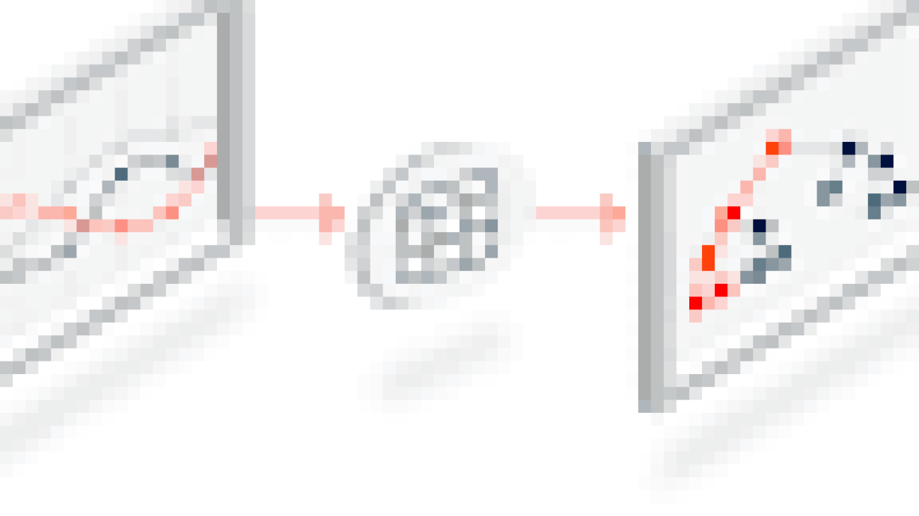
Like most neural networks, a GNN is trained on a dataset of many labeled examples (~millions), but each training step consists only of a much smaller batch of training examples (say, hundreds). To scale to millions, the GNN gets trained on a stream of reasonably small subgraphs from the underlying graph. Each subgraph contains enough of the original data to compute the GNN result for the labeled node at its center and train the model. This process — typically referred to as subgraph sampling — is extremely consequential for GNN training. Most existing tooling accomplishes sampling in a batch way, producing static subgraphs for training. TF-GNN provides tooling to improve on this by sampling dynamically and interactively.

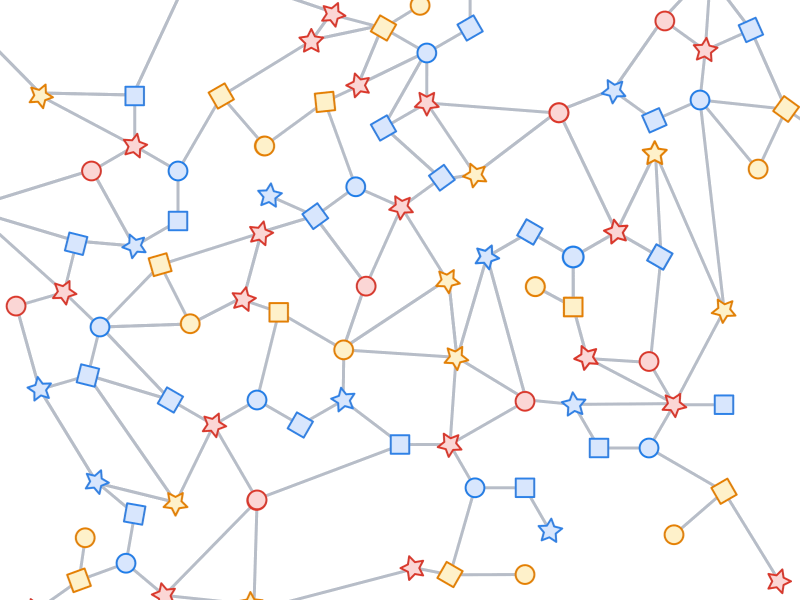
Pictured, the process of subgraph sampling where small, tractable subgraphs are sampled from a larger graph to create input examples for GNN training.

TF-GNN 1.0 debuts a flexible Python API to configure dynamic or batch subgraph sampling at all relevant scales: interactively in a Colab notebook (like this one), for efficient sampling of a small dataset stored in the main memory of a single training host, or distributed by Apache Beam for huge datasets stored on a network filesystem (up to hundreds of millions of nodes and billions of edges). For details, please refer to our user guides for in-memory and beam-based sampling, respectively.

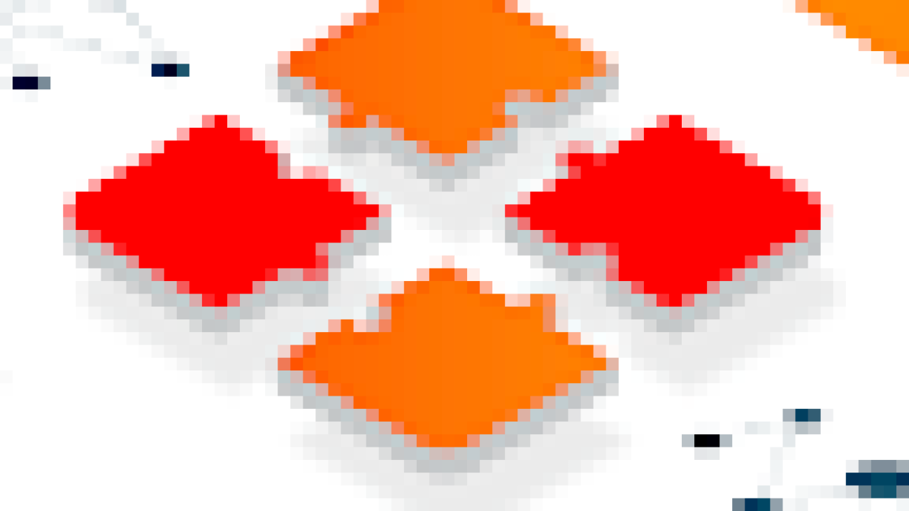
On those same sampled subgraphs, the GNN’s task is to compute a hidden (or latent) state at the root node; the hidden state aggregates and encodes the relevant information of the root node’s neighborhood. One classical approach is message-passing neural networks. In each round of message passing, nodes receive messages from their neighbors along incoming edges and update their own hidden state from them. After n rounds, the hidden state of the root node reflects the aggregate information from all nodes within n edges (pictured below for n = 2). The messages and the new hidden states are computed by hidden layers of the neural network. In a heterogeneous graph, it often makes sense to use separately trained hidden layers for the different types of nodes and edges.

Pictured, a simple message-passing neural network where, at each step, the node state is propagated from outer to inner nodes where it is pooled to compute new node states. Once the root node is reached, a final prediction can be made.

The training setup is completed by placing an output layer on top of the GNN’s hidden state for the labeled nodes, computing the loss (to measure the prediction error), and updating model weights by backpropagation, as usual in any neural network training.

Beyond supervised training (i.e., minimizing a loss defined by labels), GNNs can also be trained in an unsupervised way (i.e., without labels). This lets us compute a continuous representation (or embedding) of the discrete graph structure of nodes and their features. These representations are then typically utilized in other ML systems. In this way, the discrete, relational information encoded by a graph can be included in more typical neural network use cases. TF-GNN supports a fine-grained specification of unsupervised objectives for heterogeneous graphs.

Building GNN architectures

The TF-GNN library supports building and training GNNs at various levels of abstraction.

At the highest level, users can take any of the predefined models bundled with the library that are expressed in Keras layers. Besides a small collection of models from the research literature, TF-GNN comes with a highly configurable model template that provides a curated selection of modeling choices that we have found to provide strong baselines on many of our in-house problems. The templates implement GNN layers; users need only to initialize the Keras layers.

import tensorflow_gnn as tfgnn
from tensorflow_gnn.models import mt_albis

def model_fn(graph_tensor_spec: tfgnn.GraphTensorSpec):
  """Builds a GNN as a Keras model."""
  graph = inputs = tf.keras.Input(type_spec=graph_tensor_spec)

  # Encode input features (callback omitted for brevity).
  graph = tfgnn.keras.layers.MapFeatures(
      node_sets_fn=set_initial_node_states)(graph)

  # For each round of message passing...
  for _ in range(2):
    # ... create and apply a Keras layer.
    graph = mt_albis.MtAlbisGraphUpdate(
        units=128, message_dim=64,
        attention_type="none", simple_conv_reduce_type="mean",
        normalization_type="layer", next_state_type="residual",
        state_dropout_rate=0.2, l2_regularization=1e-5,
    )(graph)

  return tf.keras.Model(inputs, graph)

At the lowest level, users can write a GNN model from scratch in terms of primitives for passing data around the graph, such as broadcasting data from a node to all its outgoing edges or pooling data into a node from all its incoming edges (e.g., computing the sum of incoming messages). TF-GNN’s graph data model treats nodes, edges and whole input graphs equally when it comes to features or hidden states, making it straightforward to express not only node-centric models like the MPNN discussed above but also more general forms of GraphNets. This can, but need not, be done with Keras as a modeling framework on the top of core TensorFlow. For more details, and intermediate levels of modeling, see the TF-GNN user guide and model collection.

Training orchestration

While advanced users are free to do custom model training, the TF-GNN Runner also provides a succinct way to orchestrate the training of Keras models in the common cases. A simple invocation may look like this:

from tensorflow_gnn import runner

runner.run(
   task=runner.RootNodeBinaryClassification("papers", ...),
   model_fn=model_fn,
   trainer=runner.KerasTrainer(tf.distribute.MirroredStrategy(), model_dir="/tmp/model"),
   optimizer_fn=tf.keras.optimizers.Adam,
   epochs=10,
   global_batch_size=128,
   train_ds_provider=runner.TFRecordDatasetProvider("/tmp/train*"),
   valid_ds_provider=runner.TFRecordDatasetProvider("/tmp/validation*"),
   gtspec=...,
)

The Runner provides ready-to-use solutions for ML pains like distributed training and tfgnn.GraphTensor padding for fixed shapes on Cloud TPUs. Beyond training on a single task (as shown above), it supports joint training on multiple (two or more) tasks in concert. For example, unsupervised tasks can be mixed with supervised ones to inform a final continuous representation (or embedding) with application specific inductive biases. Callers only need substitute the task argument with a mapping of tasks:

from tensorflow_gnn import runner
from tensorflow_gnn.models import contrastive_losses

runner.run(
     task={
        "classification": runner.RootNodeBinaryClassification("papers", ...),
        "dgi": contrastive_losses.DeepGraphInfomaxTask("papers"),
      },
    ...
)

Additionally, the TF-GNN Runner also includes an implementation of integrated gradients for use in model attribution. Integrated gradients output is a GraphTensor with the same connectivity as the observed GraphTensor but its features replaced with gradient values where larger values contribute more than smaller values in the GNN prediction. Users can inspect gradient values to see which features their GNN uses the most.

Conclusion

In short, we hope TF-GNN will be useful to advance the application of GNNs in TensorFlow at scale and fuel further innovation in the field. If you’re curious to find out more, please try our Colab demo with the popular OGBN-MAG benchmark (in your browser, no installation required), browse the rest of our user guides and Colabs, or take a look at our paper.

Acknowledgements

The TF-GNN release 1.0 was developed by a collaboration between Google Research (Sami Abu-El-Haija, Neslihan Bulut, Bahar Fatemi, Johannes Gasteiger, Pedro Gonnet, Jonathan Halcrow, Liangze Jiang, Silvio Lattanzi, Brandon Mayer, Vahab Mirrokni, Bryan Perozzi, Anton Tsitsulin, Dustin Zelle), Google Core ML (Arno Eigenwillig, Oleksandr Ferludin, Parth Kothari, Mihir Paradkar, Jan Pfeifer, Rachael Tamakloe), and Google DeepMind (Alvaro Sanchez-Gonzalez and Lisa Wang).

Read More

Posted by the TensorFlow team

We are releasing a hot-fix for an installation issue affecting the TensorFlow installation process. The TensorFlow 2.15.0 Python package was released such that it requested tensorrt-related packages that cannot be found unless the user installs them beforehand or provides additional installation flags. This dependency affected anyone installing TensorFlow 2.15 alongside NVIDIA CUDA dependencies via pip install tensorflow[and-cuda]. Depending on the installation method, TensorFlow 2.14 would be installed instead of 2.15, or users could receive an installation error due to those missing dependencies.

To solve this issue as quickly as possible, we have released TensorFlow 2.15.0.post1 for the Linux x86_64 platform. This version removes the tensorrt Python package dependencies from the tensorflow[and-cuda] installation method. Support for TensorRT is otherwise unaffected as long as TensorRT is already installed on the system. Now, pip install tensorflow[and-cuda] works as originally intended for TensorFlow 2.15.

Using .post1 instead of a full minor release allowed us to push this release out quickly. However, please be aware of the following caveat: for users wishing to pin their Python dependency in a requirements file or other situation, under Python’s version specification rules, tensorflow[and-cuda]==2.15.0 will not install this fixed version. Please use ==2.15.0.post1 to specify this exact version on Linux platforms, or a fuzzy version specification, such as ==2.15.*, to specify the most recent compatible version of TensorFlow 2.15 on all platforms.

Read More

Posted by Marat Dukhan and Frank Barchard, Software Engineers

CPUs deliver the widest reach for ML inference and remain the default target for TensorFlow Lite. Consequently, improving CPU inference performance is a top priority, and we are excited to announce that we doubled floating-point inference performance in TensorFlow Lite’s XNNPack backend by enabling half-precision inference on ARM CPUs. This means that more AI powered features may be deployed to older and lower tier devices.

Traditionally, TensorFlow Lite supported two kinds of numerical computations in machine learning models: a) floating-point using IEEE 754 single-precision (32-bit) format and b) quantized using low-precision integers. While single-precision floating-point numbers provide maximum flexibility and ease of use, they come at the cost of 4X overhead in storage and memory and exhibit a performance overhead compared to 8-bit integer computations. In contrast, half-precision (FP16) floating-point numbers pose an interesting alternative balancing ease-of-use and performance: the processor needs to transfer twice fewer bytes and each vector operation produces twice more elements. By virtue of this property, FP16 inference paves the way for 2X speedup for floating-point models compared to the traditional FP32 way.

For a long time FP16 inference on CPUs primarily remained a research topic, as the lack of hardware support for FP16 computations limited production use-cases. However, around 2017 new mobile chipsets started to include support for native FP16 computations, and by now most mobile phones, both on the high-end and the low-end. Building upon this broad availability, we are pleased to announce the general availability for half-precision inference in TensorFlow Lite and XNNPack.

Performance Improvements

Half-precision inference has already been battle-tested in production across Google Assistant, Google Meet, YouTube, and ML Kit, and demonstrated close to 2X speedups across a wide range of neural network architectures and mobile devices. Below, we present benchmarks on nine public models covering common computer vision tasks:

1. MobileNet v2 image classification [download]
2. MobileNet v3-Small image classification [download]
3. DeepLab v3 segmentation [download]
4. BlazeFace face detection [download]
5. SSDLite 2D object detection [download]
6. Objectron 3D object detection [download]
7. Face Mesh landmarks [download]
8. MediaPipe Hands landmarks [download]
9. KNIFT local feature descriptor [download]

These models were benchmarked on 5 popular mobile devices, including recent and older devices (Pixel 3a, Pixel 5a, Pixel 7, Galaxy M12 and Galaxy S22). The average speedup is shown below.

Single-threaded inference speedup with half-precision (FP16) inference compared to single-precision (FP32) across 5 mobile devices. Higher numbers are better.

The same models were also benchmarked on three laptop computers (MacBook Air M1, Surface Pro X and Surface Pro 9)

Single-threaded inference speedup with half-precision (FP16) inference compared to single-precision (FP32) across 3 laptop computers. Higher numbers are better.

Currently, the FP16-capable hardware supported in XNNPack is limited to ARM & ARM64 devices with ARMv8.2 FP16 arithmetics extension, which includes Android phones starting with Pixel 3, Galaxy S9 (Snapdragon SoC), Galaxy S10 (Exynos SoC), iOS devices with A11 or newer SoCs, all Apple Silicon Macs, and Windows ARM64 laptops based with Snapdragon 850 SoC or newer.

How Can I Use It?

To benefit from the half-precision inference in XNNPack, the user must provide a floating-point (FP32) model with FP16 weights and special “reduced_precision_support” metadata to indicate model compatibility with FP16 inference. The metadata can be added during model conversion using the _experimental_supported_accumulation_type attribute of the tf.lite.TargetSpec object:

...
converter.target_spec.supported_types = [tf.float16]
converter.target_spec._experimental_supported_accumulation_type = tf.dtypes.float16

When the compatible model is delegated to XNNPack on a hardware with native support for FP16 computations, XNNPack will transparently replace FP32 operators with their FP16 equivalents, and insert additional operators to convert model inputs from FP32 to FP16 and convert model outputs back from FP16 to FP32. If the hardware is not capable of FP16 arithmetics, XNNPack will perform model inference with FP32 calculations. Therefore, a single model can be transparently deployed on both recent and legacy devices.

Additionally, the XNNPack delegate provides an option to force FP16 inference regardless of the model metadata. This option is intended for development workflows, and in particular for testing end-to-end accuracy of the model when FP16 inference is used. In addition to devices with native FP16 arithmetics support, forced FP16 inference is supported on x86/x86-64 devices with AVX2 extension in emulation mode: all elementary floating-point operations are computed in FP32, then converted to FP16 and back to FP32. Note that such simulation is slow and not a bit-exact equivalent to native FP16 inference, but simulates the effects of restricted mantissa precision and exponent range in the native FP16 arithmetics. To force FP16 inference, either build TensorFlow Lite with --define xnnpack_force_float_precision=fp16 Bazel option, or apply XNNPack delegate explicitly and add TFLITE_XNNPACK_DELEGATE_FLAG_FORCE_FP16 flag to the TfLiteXNNPackDelegateOptions.flags bitmask passed into the TfLiteXNNPackDelegateCreate call:

TfLiteXNNPackDelegateOptions xnnpack_options =
    TfLiteXNNPackDelegateOptionsDefault();
...
xnnpack_options.flags |= TFLITE_XNNPACK_DELEGATE_FLAG_FORCE_FP16;
TfLiteDelegate* xnnpack_delegate =
    TfLiteXNNPackDelegateCreate(&xnnpack_options);

XNNPack provides full feature parity between FP32 and FP16 operators: all operators that are supported for FP32 inference are also supported for FP16 inference, and vice versa. In particular, sparse inference operators are supported for FP16 inference on ARM processors. Therefore, users can combine the performance benefits of sparse and FP16 inference in the same model.

Future Work

In addition to most ARM and ARM64 processors, the most recent Intel processors, code-named Sapphire Rapids, support native FP16 arithmetics via the AVX512-FP16 instruction set, and the recently announced AVX10 instruction set promises to make this capability widely available on x86 platform. We plan to optimize XNNPack for these instruction sets in a future release.

Acknowledgements

We would like to thank Alan Kelly, Zhi An Ng, Artsiom Ablavatski, Sachin Joglekar, T.J. Alumbaugh, Andrei Kulik, Jared Duke, Matthias Grundmann for contributions towards half-precision inference in TensorFlow Lite and XNNPack.

Read More

Posted by the TensorFlow team

TensorFlow 2.15 has been released! Highlights of this release (and 2.14) include a much simpler installation method for NVIDIA CUDA libraries for Linux, oneDNN CPU performance optimizations for Windows x64 and x86, full availability of tf.function types, an upgrade to Clang 17.0.1, and much more! For the full release note, please check here.

TensorFlow Core

NVIDIA CUDA libraries for Linux

The tensorflow pip package has a new, optional installation method for Linux that installs necessary NVIDIA CUDA libraries through pip. As long as the NVIDIA driver is already installed on the system, you may now run pip install tensorflow[and-cuda] to install TensorFlow’s NVIDIA CUDA library dependencies in the Python environment. Aside from the NVIDIA driver, no other pre-existing NVIDIA CUDA packages are necessary. In TensorFlow 2.15, CUDA has been upgraded to version 12.2.

oneDNN CPU performance optimizations

For Windows x64 & x86 packages, oneDNN optimizations are now enabled by default on X86 CPUs. These optimizations can be enabled or disabled by setting the environment variable TF_ENABLE_ONEDNN_OPTS to 1 (enable) or 0 (disable) before running TensorFlow. To fall back to default settings, simply unset the environment variable.

tf.function

tf.function types are now fully available.

tf.types.experimental.TraceType now allows custom tf.function inputs to declare Tensor decomposition and type casting support. 

Introducing tf.types.experimental.FunctionType as the comprehensive representation of the signature of tf.function callables. It can be accessed through the function_type property of tf.function’s and ConcreteFunctions. See the tf.types.experimental.FunctionType documentation for more details. 

Introducing tf.types.experimental.AtomicFunction as the fastest way to perform TF computations in Python. This capability can be accessed through the inference_fn property of ConcreteFunctions. (Does not support gradients.) See the tf.types.experimental.AtomicFunction documentation for how to call and use it.

Upgrade to Clang 17.0.1 and CUDA 12.2

TensorFlow PIP packages are now being built with Clang 17 and CUDA 12.2 to improve performance for NVIDIA Hopper-based GPUs. Moving forward, Clang 17 will be the default C++ compiler for TensorFlow. We recommend upgrading your compiler to Clang 17 when building TensorFlow from source.

Read More

Posted by Sharbani Roy – Senior Director, Product Management, Google

The Women in ML Symposium is an inclusive event for anyone passionate about the transformative fields of Machine Learning (ML) and Artificial Intelligence (AI). Dive into the latest advancements in generative AI, explore the intricacies of privacy-preserving AI, dig into the underlying accelerators and ML frameworks that power models, and uncover practical applications of ML across multiple industries.

Our event offers sessions for all expertise levels, from beginners to advanced practitioners. Hear about what’s new in ML and building with Google AI from our keynote speakers, gain insights from seasoned industry leaders across Google Health, Nvidia, Adobe, and more – and discover a wealth of knowledge on topics ranging from foundational AI concepts to open source tools, techniques, and beyond.

RSVP today to secure your spot and explore our exciting agenda. We can’t wait to see you there!

Read More

Posted by Surya Kanoria, Joseph Cauteruccio, Federico Tomasi, Kamil Ciosek, Matteo Rinaldi, and Zhenwen Dai – Spotify

Introduction

Many of our music recommendation problems involve providing users with ordered sets of items that satisfy users’ listening preferences and intent at that point in time. We base current recommendations on previous interactions with our application and, in the abstract, are faced with a sequential decision making process as we continually recommend content to users.

Reinforcement Learning (RL) is an established tool for sequential decision making that can be leveraged to solve sequential recommendation problems. We decided to explore how RL could be used to craft listening experiences for users. Before we could start training Agents, we needed to pick a RL library that allowed us to easily prototype, test, and potentially deploy our solutions.

At Spotify we leverage TensorFlow and the extended TensorFlow Ecosystem (TFX, TensorFlow Serving, and so on) as part of our production Machine Learning Stack. We made the decision early on to leverage TensorFlow Agents as our RL Library of choice, knowing that integrating our experiments with our production systems would be vastly more efficient down the line.

One missing bit of technology we required was an offline Spotify environment we could use to prototype, analyze, explore, and train Agents offline prior to online testing. The flexibility of the TF-Agents library, coupled with the broader advantages of TensorFlow and its ecosystem, allowed us to cleanly design a robust and extendable offline Spotify simulator.

We based our simulator design on TF-Agents Environment primitives and using this simulator we developed, trained and evaluated sequential models for item recommendations, vanilla RL Agents (PPG, DQN) and a modified deep Q-Network, which we call the Action-Head DQN (AH-DQN), that addressed the specific challenges imposed by the large state and action space of our RL formulation.

Through live experiments we were able to show that our offline performance estimates were strongly correlated with online results. This then opened the door for large scale experimentation and application of Reinforcement Learning across Spotify, enabled by the technological foundations unlocked by TensorFlow and TF-Agents.

In this post we’ll provide more details about our RL problem and how we used TF-Agents to enable this work end to end.

The RL Loop and Simulated Users

In our case the reward emitted from the environment is the response of a user to music recommendations driven by the Agent’s action. In the absence of a simulator we would need to expose real users to Agents to observe rewards. We utilize a model-based RL approach to avoid letting an untrained Agent interact with real users (with the potential of hurting user satisfaction in the training process).

In this model-based RL formulation the Agent is not trained online against real users. Instead, it makes use of a user model that predicts responses to a list of tracks derived via the Agent’s action. Using this model we optimize actions in such a way as to maximize a (simulated) user satisfaction metric. During the training phase the environment makes use of this user model to return a predicted user response to the action recommended by the Agent.

We use Keras to design and train our user model. The serialized user model is then unpacked by the simulator and used to calculate rewards during Agent training and evaluation.

Simulator Design

In the abstract, what we needed to build was clear. We needed a way to simulate user listening sessions for the Agent. Given a simulated user and some content, instantiate a listening session and let the Agent drive recommendations in that session. Allow the simulated user to “react” to these recommendations and let the Agent adjust its strategy based on this result to drive some expected cumulative reward.

The TensorFlow Agents environment design guided us in developing the modular components of our system, each of which was responsible for different parts of the overall simulation.

In our codebase we define an environment abstraction that requires the following be defined for every concrete instantiation:

Set-Up

Actions and Observations

Just like any Agent environment, our simulator requires that we specify the action_spec and observation_spec. Actions in our case may be continuous or discrete depending both on our Agent selection and how we propose to translate an Agent’s action into actual recommendations. We typically recommend ordered lists of items drawn from a pool of potential items. Formulating this action space directly would lead to it being combinatorially complex. We also assume the user will interact with multiple items, and as such previous work in this area that relies on single choice assumptions doesn’t apply.

Termination and Reset

We also need to handle the episode termination dynamics. In our simulator, the reset rules are set by the model builder and based on empirical investigations of interaction data relevant to a specific music listening experience. As a hypothetical, we may determine that 92% of listening sessions terminate after 6 sequential track skips and we’d construct our simulation termination logic to match. It also requires that we design abstractions in our simulator that allow us to check if the episode should be terminated after each step.

When the episode is reset the simulator will sample a new hypothetical user listening session pair and begin the next episode.

Episode Steps

As with standard TF Agents Environments we need to define the step dynamics for our simulation. We have optional dynamics of the simulation that we need to make sure are enforced at each step. For example, we may desire that the same item cannot be recommended more than once. If the Agent’s action indicates a recommendation of an item that was previously recommended we need to build in the functionality to pick the next best item based on this action.

We also need to call the termination (and other supporting functions) mentioned above as needed at each step.

Episode Storage and Replay

The functionality mentioned up until this point collectively created a very complex simulation setup. While the TF Agents replay buffer provided us with the functionality required to store episodes for Agent training and evaluation, we quickly realized the need to be able to store more episode data for debugging purposes, and more detailed evaluations specific to our simulation distinct from standard Agent performance measures.

We thus allowed for the inclusion of an expanded _episode_tracker that would store additional information about the user model predictions, information noting the sampled users/content pairs, and more.

Creating TF-Agent Environments

Our environment abstraction gives us a template that matches that of a standard TF-Agents Environment class. Some inputs to our environment need to be resolved before we can actually create the concrete TF-Agents environment instance. This happens in three steps.

First we define a specific simulation environment that conforms to our abstraction. For example:

Next we use an Environment Builder Class that takes as input a user model, track sampler, etc. and an environment class like PlaylistEnvironment. The builder creates a concrete instance of this environment:

Lastly, we utilize a conversion class that constructs a TF-Agents Environment from a concrete instance of ours:

class TFAgtPyEnvironment(py_environment.PyEnvironment):     def __init__(self, environment: AbstractEnvironment):   super().__init__()   self.env = environment

This is then executed internally to our Environment Builder:

class EnvironmentBuilder(AbstractEnvironmentBuilder):       def __init__(self, ...):       ...       def get_tf_env(self):        ...       tf_env: TFAgtPyEnvironment = TFAgtPyEnvironment(     self.playlist_env       )       return tf_env

The resulting TensorFlow Agents environment can then be used for Agent training.

This simulator design allows us to easily create and manage multiple environments with a variety of different configurations as needed.

We next discuss how we used our simulator to train RL Agents to generate Playlists.

A Customized Agent for Playlist Generation

As mentioned, Reinforcement Learning provides us with a method set that naturally accommodates the sequential nature of music listening; allowing us to adapt to users’ ever evolving preferences as sessions progress.

One specific problem we can attempt to use RL to solve is that of automatic music playlist generation. Given a (large) set of tracks, we want to learn how to create one optimal playlist to recommend to the user in order to maximize satisfaction metrics. Our use case is different from standard slate recommendation tasks, where usually the target is to select at most one item in the sequence. In our case, we assume we have a user-generated response for multiple items in the slate, making slate recommendation systems not directly applicable. Another complication is that the set of tracks from which recommendations are drawn is ever changing.

We designed a DQN variant capable of handling these constraints that we called an Action Head DQN (AHDQN).

The AH-DQN network takes as input the current state and an available action to produce a single Q value for the input action. This process is repeated for every possible item in the input. Finally, the item with the highest Q value is selected and added to the slate, and the process continues until the slate is full.

Experiments In Brief

We tested our approach both offline and online at scale to assess the ability of the Agent to power our real-world recommender systems. In addition to testing the Agent itself we were also keen to assess the extent to which our offline performance estimates for various policies returned by our simulator matched (or at least directionally aligned) with our online results.

We observed this directional alignment for numerous naive, heuristic, model driven, and RL policies.

Please refer to our KDD paper for more information on the specifics of our model-based RL approach and Agent design.

Automatic Music Playlist Generation via Simulation-based Reinforcement Learning

Federico Tomasi, Joseph Cauteruccio, Surya Kanoria, Kamil Ciosek, Matteo Rinaldi, and Zhenwen Dai

KDD 2023

Acknowledgements

We’d like to thank all our Spotify teammates past and present who contributed to this work. Particularly, we’d like to thank Mehdi Ben Ayed for his early work in helping to develop our RL codebase. We’d also like to thank the TensorFlow Agents team for their support and encouragement throughout this project (and for the library that made it possible).

Read More

Posted by Wei Wei, Developer Advocate

In our previous blog posts Building a board game app with TensorFlow: a new TensorFlow Lite reference app and Building a reinforcement learning agent with JAX, and deploying it on Android with TensorFlow Lite, we demonstrated how to train a reinforcement learning (RL) agent with TensorFlow, TensorFlow Agents and JAX respectively, and then deploy the converted TFLite model in an Android app using TensorFlow Lite, to play a simple board game ‘Plane Strike’.

Since we already have the model trained with TensorFlow and converted to TFLite, we can just load the model with TFLite interpreter:

That’s it! With some additional Flutter frontend code to render the game boards and track game progress, we can immediately run the game on both Android and iOS (currently the plugin only supports these two mobile platforms). You can find the complete code on GitHub.

Convert the TFAgents-trained model to TFLite and run it with the plugin

Leverage the RL technique we have used and build a new agent for the tic tac toe game in the Flutter Casual Games Toolkit. You will need to create a new RL environment and train the model from scratch before deployment, but the core concept and technique are pretty much the same.

This concludes this mini-series of blogs on leveraging TensorFlow/JAX to build games for Android and Flutter. And we very much look forward to all the exciting things you build with our tooling, so be sure to share them with @googledevs, @TensorFlow, and your developer communities!

Read More

Posted by Ashley Oldacre

If you are joining us for the first time, you can binge listen to our amazing 8 episodes from Season 1 wherever you get your podcasts.

We are back for another season of People of AI with a new lineup of incredible guests! I am so excited to introduce my new co-host Luiz Gustavo Martins as we meet inspiring people with interesting stories in the field of Artificial Intelligence.

Last season we focused on the incredible journeys that our guests took to get into the field of AI. Through our stories, we highlighted that no matter who you are, what your interests are, or what you work on, there is a place for anyone to get into this field. We also explored how much more accessible the technology has become over the years, as well as the importance of building AI-related products responsibly and ethically. It is easier than ever to use tools, platforms and services powered by machine learning to leverage the benefits of AI, and break down the barrier of entry.

For season 2, we will feature amazing conversations, focusing on Generative AI! Specifically, we will be discussing the explosive growth of Generative AI tools and the major technology shift that has happened in recent months. We will dive into various topics to explore areas where Generative AI can contribute tremendous value, as well as boost both productivity and economic growth. We will also continue to explore the personal paths and career development of this season’s guests as they share how their interest in technology was sparked, how they worked hard to get to where they are today, and explore what it is that they are currently working on.

Starting today, we will release one new episode of season 2 per week. Listen to the first episode on the People of AI site or wherever you get your podcasts. And stay tuned for later in the season when we premiere our first video podcasts as well!

Episode 1: meet your hosts, Ashley and Gus and learn about Generative AI, Bard and the big shift that has dramatically changed the industry. 

Episode 2: meet Sunita Verma, a long-time Googler, as she shares her personal journey from Engineering to CS, and into Google. As an early pioneer of AI and Google Ads, we will talk about the evolution of AI and how Generative AI will transform the way we work. 

Episode 3: meet Sayak Paul, a Google Developer Expert (GDE) as we explore what it means to be a GDE and how to leverage the power of your community through community contributions. 

Episode 4: meet Crispin Velez, the lead for Cloud’s Vertex AI as we dig into his experience in Cloud working with customers and partners on how to integrate and deploy AI. We also learn how he grew his AI developer community in LATAM from scratch. 

Episode 5: meet Joyce Shen, venture capital/private equity investor. She shares her fascinating career in AI and how she has worked with businesses to spot AI talent, incorporate AI technology into workflows and implement responsible AI into their products. 

Episode 6: meet Anne Simonds and Brian Gary, founders of Muse https://www.museml.com. Join us as we talk about their recent journeys into AI and their new company which uses the power of Generative AI to spark creativity. 

Episode 7: meet Tulsee Doshi, product lead for Google’s Responsible AI efforts as we discuss the development of Google-wide resources and best practices for developing more inclusive, diverse, and ethical algorithm driven products. 

Episode 8: meet Jeanine Banks, Vice President and General Manager of Google Developer X and Head of Developer Relations. Join us as we debunk AI and get down to what Generative AI really is, how it has changed over the past few months and will continue to change the developer landscape. 

Episode 9: meet Simon Tokumine, Director of Product Management at Google. We will talk about how AI has brought us into the era of task-orientated products and is fueling a new community of makers.

Listen now to the first episode of Season 2. We can’t wait to share the stories of these exceptional People of AI with you!

This podcast is sponsored by Google. Any remarks made by the speakers are their own and are not endorsed by Google.

Read More