AI and Machine Learning @ I/O Recap

AI and Machine Learning @ I/O Recap

Posted by Lauren Usui and Joe Fernandez

Artificial intelligence is a topic of kitchen table conversations around the world today, and as AI becomes more accessible for users and developers, we want to make it easier and more useful for everyone. This year at Google I/O, we highlighted how we are helping developers like you build with generative AI, use machine learning in spreadsheets and applications, create ML models from the ground up, and scale them up to serve millions of users.

While AI technology is advancing rapidly, we must continue to ensure it is used responsibly. So we also took some time to explain how Google is taking a principled approach to applying generative AI and how you can apply our guidelines and tools to make sure your AI-powered products and projects are built responsibly to serve all your users.

If you are new to AI and want to get a quick overview of the technology, check out the getting started video from Google’s AI advocate lead, Laurence Moroney.

Develop generative AI apps with PaLM 2

Everyone seems to be chatting with—or about—generative AI recently, and we want you to be able to use Google’s latest large language model, PaLM 2, to power new and helpful experiences for your users with the PaLM API. Our session on Generative AI reveals more about how you can easily prompt models with MakerSuite to quickly prototype generative AI applications. We demonstrate how you can use the PaLM API for prompting using examples, conversational chat interactions, and using embedding functionality to compress and compare text data in useful ways. We also showed off how to use the PaLM API in Google Colab notebooks with a simple, magical syntax. Check out this talk and sign up to request access to the PaLM API and MakerSuite!

Crunch numbers with AI-powered spreadsheets

Hundreds of millions of people use spreadsheets to organize, manage, and analyze data for everything from business transactions, to inventory accounting, to family budgets. We’re making it easy for everyone to bring the power of AI into spreadsheets with Simple ML for Sheets, a Google Sheets add-on. We recently updated this tool to include anomaly detection and forecasting features. Check out the demonstration of how to predict missing data values and forecast sales with the tool. No coding required!

Simplify on-device ML applications with MediaPipe

AI is finding its way into applications across multiple platforms and MediaPipe makes it easy to build, customize, and deploy on-device ML solutions. We upgraded MediaPipe Solutions this year, improving existing solutions and adding new ones, including interactive segmentation to blur the background behind a selected subject and face stylization to render that selfie in your favorite graphic style.

Do more with Web ML

Every week, hundreds of thousands of developers build AI-powered applications to run in the browser or Node.js using JavaScript and web technologies. Web ML has advanced in multiple areas, and we provide a round up of the top updates in this year’s I/O talk. We announced Visual Blocks for ML, an open JavaScript framework for quickly and interactively building custom ML pipelines. You can now run machine learning models even faster with improved WebGL performance and the release of WebGPU in Chrome. More tools and resources are also now available for web ML developers, including TensorFlow Decision Forest support, a visual debugger for models, JAX to JS conversion support, and a new Zero to Hero training course to grow your skills in Web ML.

Find pre-trained models fast with Kaggle Models

Building machine learning models can take a huge amount of time and effort: collecting data, training, evaluating, and optimizing. Kaggle is making it a whole lot easier for developers to discover and use pretrained models. With Kaggle Models, you can search thousands of open-licensed models from leading ML researchers for multiple ML platforms. Find the model you need quickly with filters for tasks, supported data types, model architecture, and more. Combine this new feature with Kaggle’s huge repository of over 200K datasets and accelerate your next ML project.

Apply ML to vision and text with Keras

Lots of developers are exploring AI technologies and many of you are interested in working on computer vision and natural language processing applications. Keras released new, easy-to-use libraries for computer vision and natural language processing with KerasCV and KerasNLP. Using just a few lines of code, you can apply the latest techniques and models for data augmentation, object detection, image and text generation, and text classification. These new libraries provide modular implementations that are easy to customize and are tightly integrated with the broader TensorFlow ecosystem including TensorFlow Lite, TPUs, and DTensor.

Build ML flexibly and scalably with TensorFlow

With one of the largest ML development communities in the world, the TensorFlow ecosystem helps hundreds of thousands of developers like you build, train, deploy, and manage machine learning models. ML technology is rapidly evolving, and we’re upgrading TensorFlow with new tools to give you more flexibility, scalability, and efficiency. If you’re using JAX, you can now bring your model components into the TensorFlow ecosystem with JAX2TF. We also improved DTensor support for model parallelization, allowing you to scale up execution of larger models by running portions of a single model, or shards, across multiple machines. We also announced a toolkit for applying quantization techniques to practically any TensorFlow model, helping you gain substantial efficiency improvements for your AI applications. The quantization toolkit will be available later this year.

Scale large language models with Google Cloud

When it’s time to deploy your AI-powered applications to your business, enterprise, or the world, you need reliable tools and services that scale with you. Google Cloud’s Vertex AI is an end-to-end ML platform that helps you develop ML models quickly and easily, and deploy them at any scale. To help you build generative AI technology for your product or business, we’ve introduced Model Garden and the Generative AI Studio as part of the Vertex AI platform. Model Garden gives you quick access to the latest foundation models such as Google PaLM 2, and many more to build AI-powered applications for text processing, imagery, and code. Generative AI Studio lets you quickly prototype generative AI applications right in your browser, and when you are ready to deploy, Vertex AI and Google Cloud services enable you to scale up to hundreds, thousands, or millions of users.

Explore new resources to build with Google AI

As tools, technology, and techniques for AI development rapidly advance, finding what you need to get started or take the next step with your project can be challenging. We’re making it easier to find the right resources to accelerate your AI development at Build with Google AI. This new site brings together tools, guidance, and community for building, deploying, and managing ML. Whether you are creating AI for on-device apps or deploying AI at scale, we help you navigate the options and find your path. Check out our latest toolkits on Building an LLM on Android and Text Classification with Keras.

Making Generative AI safe and responsible

AI is a powerful tool, and it’s up to all of us to ensure that it is used responsibly and for the benefit of all. We’re committed to ensuring Google’s AI systems are developed according to our AI principles. This year at Google I/O, we shared how we’ve created guidelines and tools for building generative AI safely and responsibly, and how you can apply those same guidelines and tools for your own projects.

Aaannnd that’s a wrap! Check out the full playlist of all the AI-related sessions we mentioned above. We are excited to share these new tools, resources, and technologies with you, and we can’t wait to see what you build with them!

Read More

Google I/O 2023: What’s new in TensorFlow and Keras?

Google I/O 2023: What’s new in TensorFlow and Keras?

Posted by Ayush Jain, Carlos Araya, and Mani Varadarajan for the TensorFlow team

Welcome to TensorFlow and Keras at Google I/O!

The world of machine learning is changing, faster than ever. The rise of Large Language Models (LLMs) is sparking the imagination of developers worldwide, with new generative AI applications reaching hundreds of millions of people around the world. These models are trained on massive datasets, and used to solve a variety of tasks, from natural language processing to image generation.

Powering all these new capabilities requires new levels of model efficiency and performance, as well as support for seamless deployment across a growing number of devices – be it on a server, the web, mobile devices, or beyond. As stewards of one of the largest machine learning communities in the world, the TensorFlow team is continually asking how we can better serve you.

To that end, this post covers a few of the many improvements and additions coming this year to the TensorFlow ecosystem. Let’s dive in!

A Growing Ecosystem

New functionality we’re covering today:

KerasCV and KerasNLP allows you to access pre-trained, state-of-the-art models in just a few lines of code.

DTensor helps you scale up your models and train them efficiently by combining different parallelism techniques.

With JAX2TF, models written with the JAX numerical library can be used in the TensorFlow ecosystem.

We also preview the TF Quantization API, which enables you to make your models more cost and resource-efficient without compromising on accuracy.

Applied ML with KerasCV & KerasNLP

KerasCV and KerasNLP are powerful, modularized libraries that give you direct access to the state-of-the-art in computer vision and natural language processing.

The KerasCV + KerasNLP suite, at a glance.

Whether you want to classify images, auto-generate text from prompts like with Bard or anything in between, KerasCV and KerasNLP make it easy with just a few lines of code. And since it’s a part of Keras, it’s fully integrated with the TensorFlow Ecosystem.

Let’s look at some code for image generation. KerasCV is designed to support many models, and in this case we’ll use a diffusion model. Despite the complexity of the underlying architecture, you can get it up and running with just a few lines of code.

from keras_cv.models import (
StableDiffusion,
)

model = StableDiffusion(
img_width=512,
img_height=512,
)

With one line to import and another to initialize the model, you can generate completely new images:

images = model.text_to_image(
"photograph of an astronaut "
"riding a horse",
batch_size=3,
)
KerasCV-generated images of an astronaut riding a horse
KerasCV-generated images of an astronaut riding a horse!

This is just one of many examples. To learn more, check out our full talk on KerasCV and KerasNLP or in-depth toolkit guides at keras.io/keras_cv and keras.io/keras_nlp.

Machine Learning at Scale with DTensor

DTensor enables larger and more performant model training by giving developers the flexibility to combine and fine-tune multiple parallelism techniques.

Traditionally, ML developers have scaled up models through data parallelism, which splits up your data and feeds it to horizontally-scaled model instances. This scales up training but has an important limitation: it requires that the model fits within a single hardware device.

As models get bigger, fitting into a single device is no longer a guarantee — developers need to be able to scale their models across hardware devices. This is where model parallelism becomes important, allowing for the model to be split up into shards that can be trained in parallel.

With DTensor, data and model parallelism are not only supported, but also can be directly combined to scale models even more efficiently. And it’s completely accelerator agnostic — whether you use TPUs, GPUs, or something else.

Diagram illustrating mixed (data + model) parallelism, with DTensor.
Mixed (data + model) parallelism, with DTensor.

Let’s go through an example. Let’s say that you are building with a transformer model, like the Open Pre-trained Transformer (OPT) available through KerasNLP, and training it with some input dataset:

opt_lm = keras_nlp.models.OPTCasualLM.from_preset("opt_6.7b_en")
opt_lm.compile(...)
opt_lm.fit(wiki_text_dataset)

But here’s the thing about OPT — it’s big. With variations up to 175 billion parameters, if we tried traditional data parallelism, it would have errored outright — there’s just too many weights to reasonably replicate within a single hardware device. That’s where DTensor comes in.

To work with DTensor, we need to define two things:

First is a mesh, where you define (a) a set of hardware devices and (b) a topology, here the batch and model dimensions.

mesh_dims = [("batch", 2), ("model", 4)] mesh = dtensor.create_distributed_mesh(mesh_dims, device_type="GPU")
dtensor.initialize_accelerator_system("GPU")

Second is a layout, which defines how to shard the Tensor dimension on your defined mesh. Through our Keras domain package integrations, you can do this in just one line.

layout_map = keras_nlp.models.OPTCausalLM.create_layout_map(mesh)

From there, you create the DTensor layout’s context and include your model creation code within it. Note that at no point did we have to make any changes to the model itself!

with layout_map.scope():
opt_lm = keras_nlp.models.OPTCasualLM.from_preset("opt_6.7b_en")
opt_lm.compile(...)
opt_lm.fit(wiki_text_dataset)

Performance for DTensor today is already on par with industry benchmarks, nearly matching the gold-standard implementation of model parallelism offered by NVIDIA’s Megatron for GPUs. Further improvements are in the works to raise the bar even further, across hardware devices.

In the future, DTensor will be fully integrated with key interfaces like tf.distribute and Keras as a whole, with one entry point regardless of hardware and a number of other quality of life features. If you want to learn more, check out the DTensor overview or the Keras integration guide!

Bringing Research to Production with JAX2TF

Many of the ML advancements that are now household names had their beginnings in research. For example, the Transformer architecture, created and published by Google AI, underpins the fantastic advances in language models.

JAX has emerged as a trusted tool for much of this kind of discovery, but productionizing it is hard. To that end, we’ve been thinking about how to bring research more easily into TensorFlow, giving innovations built on JAX the full strength of TensorFlow’s uniquely robust and diverse production ecosystem.

That’s why we’ve built JAX2TF, a lightweight API that provides a pathway from the JAX ecosystem to the TensorFlow ecosystem. There are many examples of how this can be useful – here’s just a few:

  • Inference: Taking a model written for JAX and deploying it either on a server using TF Serving or on-device using TFLite.
  • Fine Tuning: Taking a model that was trained using JAX, we can bring its components to TF using JAX2TF, and continue training it in TensorFlow with your existing training data and setup.
  • Fusion: Combining parts of models that were trained using JAX with those trained using TensorFlow for maximum flexibility.

The key to enabling this kind of interoperation between JAX and TensorFlow is baked into jax2tf.convert, which takes in model components created on top of JAX (e.g. your loss function, prediction function, etc.) and creates equivalent representations of them as TensorFlow functions, which can then be exported as a TensorFlow SavedModel.

We’ve created a code walkthrough for one of the examples above: a quick fine-tuning setup, creating a simple model using modeling libraries in the JAX ecosystem (like Flax and Optax) and bringing it into TF to finish training. Check it out here.

JAX2TF is already baked into various tools in the TensorFlow ecosystem, under the hood. For example, here are code guides for simple conversion from JAX to TFLite for mobile devices and from JAX to TF.js for web deployment!

Coming Soon: The TensorFlow Quantization API

ML developers today face a wide variety of real-world constraints introduced by the settings they’re working in, like the size of a model or where it gets deployed.

With TensorFlow, we want developers to be able to quickly adjust and accommodate for these kinds of constraints, and to do so without sacrificing model quality. To do this, we’re building the TF Quantization API, a native quantization toolkit for TF2 which will be available publicly later in 2023.

Briefly, quantization is a group of techniques designed to make models faster, smaller, and generally less resource- and infrastructure-intensive to train and serve.

Quantization does this by reducing the precision of a model’s parameters, just like reducing pixel depth in an image like the one of Albert Einstein below. Note that even with reduced precision, we can still make out the key details:

Eight renderings of a photograph of Albert Einstein with increasingly reduced bit precision from 8-bit to 1-bit.
Renderings of a photograph of Albert Einstein with increasingly reduced bit precision.

At a high level, this works by taking a range of values in your starting precision, and mapping that range to a single bucket in your ending precision. Let’s illustrate this with an example:

Graph showing quantizing float representation to 4-bit integers
Quantizing float representation to 4-bit integers.

Take a look at the range [0.27, 0.49] on the x-axis: for float32, the blue line actually represents 7381976 unique numbers! The red line represents the int4 quantization of this range, condensing all of those numbers into a single bucket: 1001 (the number 9 in decimal).

By lowering precision through quantization, we can store model weights in a much more efficient, compressed form.

There’s a few different ways to quantize.

  • Post-Training Quantization (PTQ): Convert to a quantized model after training. This is as simple as it gets and most readily accessible, but there can be a small quality drop.
  • Quantization-Aware Training (QAT): Simulate quantization during just the forward pass, providing for maximal flexibility with a minimal quality tradeoff.
  • Quantized Training: Quantize all computations while training. This is still nascent, and needs a lot more testing, but is a powerful tool we want to make sure TensorFlow users have access to.

TensorFlow previously has had a few tools for developers to quantize their models, like this guide for PTQ and this one for QAT. However, these have been limited – with PTQ depending on conversion to TFLite for mobile deployment and QAT requiring you to rewrite your model.

The TF Quantization API is different – it’s designed to work regardless of where you’re deploying, and without you having to rewrite a single line of existing modeling code. We’re building it with flexibility and fidelity in mind, so you get the benefits of a smaller quantized model with new levels of fine-grained control and without any concerns about how it’ll all fit into your stack.

Since you’ve made it this far into the blog, here’s a sneak peek at how it’ll look. We’ll start with a typical setup for a TensorFlow model, just a few layers in Keras. From there, we can load in a predefined quantization schema to apply as a config map to our model.

# Step 1: Define your model, just like always.
model = tf.keras.models.Sequential([
tf.keras.layers.Conv2D(32, 3, strides=1, padding='same', activation='relu'),
… …])

# Step 2: Set up the quantization config, using a predefined schema.
scheme = scheme_registry.get_scheme('pixel_8bit_qat')
config_map = QuantizationConfigurationMap(scheme)

But if you need more flexibility, TF Quantization API will also let you fully customize how you quantize. There’s built-in support for you to curate your schema to apply different behaviors for every layer, operation, or tensor!

# ...or just as easily configure your own, whether per-layer:
layer_config = LayerConfiguration(
weight_config=..., activation_config=...)
config_map.set_config(model.layers[0], layer_config)

# per-op:
config_map.set_config(model.layers[0], op_type='matmul', config={
'a': ..., 'b': ...,
'return': ...
})

# even per-tensor:
_8bit_moving_average = QuantizationConfiguration(...)
per_tensor_config = LayerConfiguration(
weight_config=..., activation_config=_8bit_moving_average)
config_map.set_config(model.layers[0], per_tensor_config)

With that, we can directly apply quantization and train or save within a quantization context. Our model still has natural compatibility with the rest of the TF ecosystem, where quantization truly bears fruit.

# Now you can generate a quantization-aware model!
tf.quantization.apply_quantization_on_model(model, config_map, …)

# From here, you can train and save just as always.
with tf.quantization.scope(config_map):
model.fit()
model.save()

# You can also export to TFLite, without any changes!
converter = tf.lite.TFLiteConverter.from_keras_model(model)
converter.optimizations = [tf.lite.Optimize.DEFAULT] tflite_model = converter.convert()

We ran a bunch of tests using the MobileNetV2 model on the Pixel 7, and saw up to 16.7x gains in serving throughput versus the non-quantized baseline. This gain comes without any noticeable detriment to quality: both the float32 baseline and the int8 quantized model reported 73% accuracy.

The TF Quantization API isn’t public just yet, but will be available very soon and will continue to evolve to provide even more benefits.

That’s a wrap!

Today, we’ve shown you just a few of the key things we’ve been working on, and there’s a lot more to come.

We can’t wait to see what you’ll build, and we’re always inspired by our community’s enduring enthusiasm and continued partnership. Thanks for stopping by!

Acknowledgements

Special thanks to George Necula, Francois Chollet, Jonathan Bischof, Scott Zhu, Martin Gorner, Dong Li, Adam Koch, Bruce Fontaine, Laurence Moroney, Josh Gordon, Lauren Usui, and numerous others for their contributions to this post.

Read More

Scaling deep retrieval with TensorFlow Recommenders and Vertex AI Matching Engine

Posted by Jeremy Wortz, ML specialist, Google Cloud & Jordan Totten, Machine Learning Specialist

Cross posted from Google Cloud AI & Machine Learning

In a previous blog, we outlined three approaches for implementing recommendation systems on Google Cloud, including (1) a fully managed solution with Recommendations AI, (2) matrix factorization from BigQuery ML, and (3) custom deep retrieval techniques using two-tower encoders and Vertex AI Matching Engine. In this blog, we dive deep into option (3) and demonstrate how to build a playlist recommendation system by implementing an end-to-end candidate retrieval workflow from scratch with Vertex AI. Specifically, we will cover:

All related code can be found in this GitHub repository.

Background

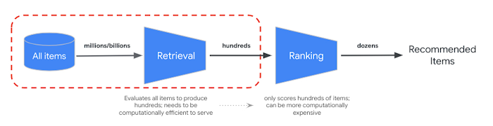
To meet low latency serving requirements, large-scale recommenders are often deployed to production as multi-stage systems. The goal of the first stage (candidate retrieval) is to sift through a large (>100M elements) corpus of candidate items and retrieve a relevant subset (~hundreds) of items for downstream ranking and filtering tasks. To optimize this retrieval task, we consider two core objectives:

  1. During model training, find the best way to compile all knowledge into query, candidate embeddings.
  2. During model serving, retrieve relevant items fast enough to meet latency requirements
Conceptual components of multi-stage recommendation systems; the focus of this blog is the first stage, candidate retrieval.
Figure 1: Conceptual components of multi-stage recommendation systems; the focus of this blog is the first stage, candidate retrieval.

Two-tower architectures are popular for retrieval tasks because they capture the semantics of query and candidate entities, and map these to a shared embedding space such that semantically similar entities cluster closer together. This means, if we compute the vector embeddings of a given query, we can search the embedding space for the closest (most similar) candidates. Because these neural network-based retrieval models take advantage of metadata, context, and feature interactions, they can produce highly informative embeddings and offer flexibility to adjust for various business objectives.

Moving image illustrating how a two tower encoder model trains, calculates, and retrieves data from the embedding space
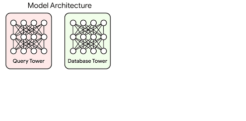
Figure 2: The two-tower encoder model is a specific type of embedding-based search where one deep neural network tower produces the query embedding and a second tower computes the candidate embedding. Calculating the dot product between the two embedding vectors determines how close (similar) the candidate is to the query. Source: Announcing ScaNN: Efficient Vector Similarity Search.

While these capabilities help achieve useful query, candidate embeddings, we still need to resolve the retrieval latency requirements. To this end, the two-tower architecture offers one more advantage: the ability to decouple inference of query and candidate items. This decoupling means all candidate item embeddings can be precomputed, reducing the serving computation to (1) converting queries to embedding vectors and (2) searching for similar vectors (among the precomputed candidates).

As candidate datasets scale to millions (or billions) of vectors, the similarity search often becomes a computational bottleneck for model serving. Relaxing the search to approximate distance calculations can lead to significant latency improvements, but we need to minimize negatively impacting search accuracy (i.e., relevance, recall).

In the paper Accelerating Large-Scale Inference with Anisotropic Vector Quantization, Google Researchers address this speed-accuracy tradeoff with a novel compression algorithm that, compared to previous state-of-the-art methods, improves both the relevance and speed of retrieval. At Google, this technique is widely-adopted to support deep retrieval use cases across Search, YouTube, Ads, Lens, and others. And while it’s available in an open-sourced library (ScaNN), it can still be challenging to implement, tune, and scale. To help teams take advantage of this technology without the operational overhead, Google Cloud offers these capabilities (and more) as a managed service with Vertex AI Matching Engine.

The goal of this post is to demonstrate how to implement these deep retrieval techniques using Vertex AI and discuss the decisions and trade-offs teams will need to evaluate for their use cases.

Reference architecture for two-tower training and deployment on Vertex AI.
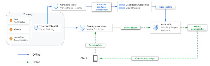
Figure 3: Figure 3: A reference architecture for two-tower training and deployment on Vertex AI.

Two-towers for deep retrieval

To better understand the benefits of two-tower architectures, let’s review three key modeling milestones in candidate retrieval.

Evolution of retrieval modeling

Traditional information retrieval systems rely heavily on token-based matching, where candidates are retrieved using an inverted index of n-grams. These systems are interpretable, easy to maintain (e.g., no training data), and are capable of achieving high precision. However, they typically suffer poor recall (i.e., trouble finding all relevant candidates for a given query) because they look for candidates having exact matches of key words. While they are still used for select Search use cases, many retrieval tasks today are either adapted with or replaced by embedding-based techniques.

Flow chart illustrating token based retrieval
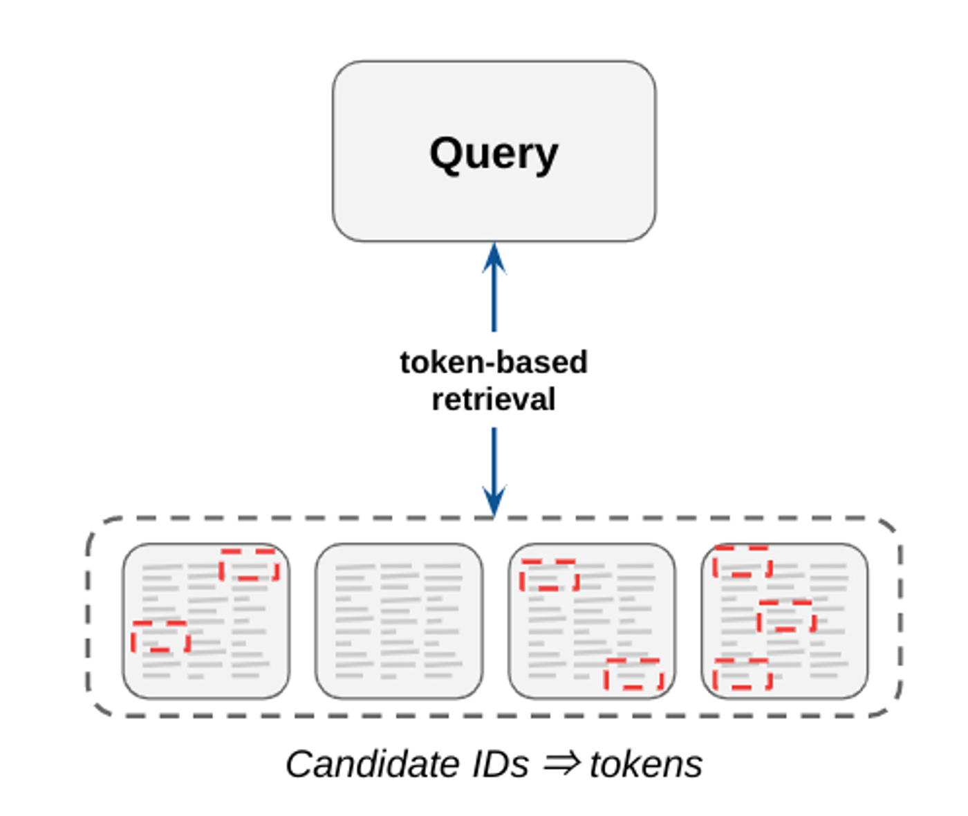
Figure 4: Token-based matching selects candidate items by matching key words found in both query and candidate items.

Factorization-based retrieval introduces a simple embedding-based model that offers much better generalization by capturing the similarity between query, candidate pairs and mapping them to a shared embedding space. One of the major benefits to this collaborative filtering technique is that embeddings are learned automatically from implicit query-candidate interactions. Fundamentally, these models factorize the full query-candidate interaction (co-occurrence) matrix to produce smaller, dense embedding representations of queries and candidates, where the product of these embedding vectors is a good approximation of the interaction matrix. The idea is that by compacting the full matrix into k dimensions the model learns the top k latent factors describing query, candidate pairs with respect to the modeling task.

Illustration of how a factorization based model factoizes a query-candidate interaction matrix intothe product of two lower rank matrices
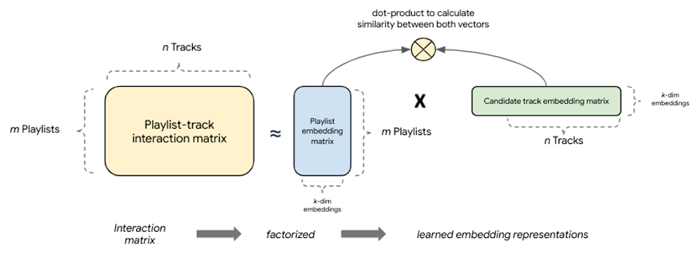
Figure 5: Factorization-based models factorize a query-candidate interaction matrix into the product of two lower-rank matrices that capture the query-candidate interactions.

The latest modeling paradigm for retrieval, commonly referred to as neural deep retrieval (NDR), produces the same embedding representations, but uses deep learning to create them. NDR models like two-tower encoders apply deep learning by processing input features with successive network layers to learn layered representations of the data. Effectively, this results in a neural network that acts as an information distillation pipeline, where raw, multi-modal features are repeatedly transformed such that useful information is magnified and irrelevant information is filtered. This results in a highly expressive model capable of learning non-linear relationships and more complex feature interactions.

Side-by-side illustrations showing the differences between factorization based retrieval and neural deep retreival
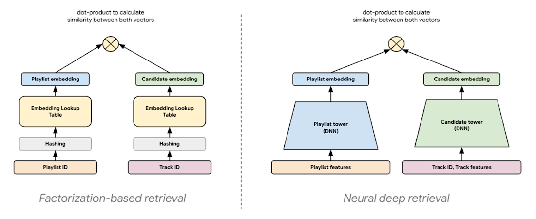
Figure 6: NDR architectures like two-tower encoders are conceptually similar to factorization models. Both are embedding-based retrieval techniques computing lower-dimensional vector representations of query and candidates, where the similarity between these two vectors is determined by computing their dot product.

In a two-tower architecture, each tower is a neural network that processes either query or candidate input features to produce an embedding representation of those features. Because the embedding representations are simply vectors of the same length, we can compute the dot product between these two vectors to determine how close they are. This means the orientation of the embedding space is determined by the dot product of each query, candidate pair in the training examples.

Decoupled inference for optimal serving

In addition to increased expressivity and generalization, this kind of architecture offers optimization opportunities for serving. Because each tower only uses its respective input features to produce a vector, the trained towers can be operationalized separately. Decoupling inference of the towers for retrieval means we can precompute what we want to find when we encounter its pair in the wild. It also means we can optimize each inference task differently:

  • Run a batch prediction job with a trained candidate tower to precompute embedding vectors for all candidates, attach NVIDIA GPU to accelerate computation
  • Compress precomputed candidate embeddings to an ANN index optimized for low-latency retrieval; deploy index to an endpoint for serving
  • Deploy trained query tower to an endpoint for converting queries to embeddings in real time, attach NVIDIA GPU to accelerate computation

Training two-tower models and serving them with an ANN index is different from training and serving traditional machine learning (ML) models. To make this clear, let’s review the key steps to operationalize this technique.

Side-by-side illustrations showing the differences between factorization based retrieval and neural deep retreival
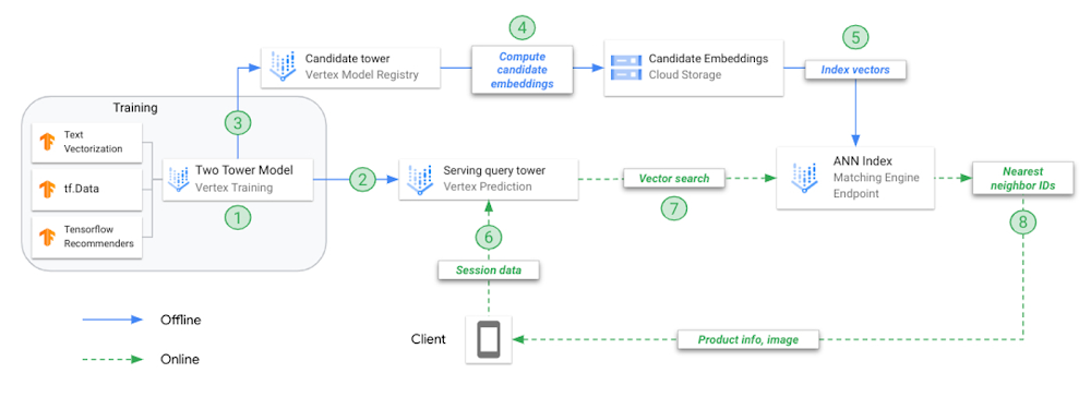
Figure 7: A reference architecture for two-tower training and deployment on Vertex AI.
  1. Train combined model (two-towers) offline; each tower is saved separately for different tasks
  2. Upload the query tower to Vertex AI Model Registry and deploy to an online endpoint
  3. Upload the candidate tower to Vertex AI Model Registry
  4. Request candidate tower to predict embeddings for each candidate track, save embeddings in JSON file
  5. Create ANN serving index from embeddings JSON, deploy to online index endpoint
  6. User application calls endpoint.predict() with playlist data, model returns the embedding vector representing that playlist
  7. Use the playlist embedding vector to search for N nearest neighbors (candidate tracks)
  8. Matching Engine returns the product IDs for the N nearest neighbors

Problem Framing

In this example, we use MPD to construct a recommendation use case, playlist continuation, where candidate tracks are recommended for a given playlist (query). This dataset is publicly available and offers several benefits for this demonstration:

  • Includes real relationships between entities (e.g., playlists, tracks, artists) which can be difficult to replicate
  • Large enough to replicate scalability issues likely to occur in production
  • Variety of feature representations and data types (e.g., playlist and track IDs, raw text, numerical, datetime); ability to enrich dataset with additional metadata from the Spotify Web Developer API
  • Teams can analyze the impact of modeling decisions by listening to retrieved candidate tracks (e.g., generate recommendations for your own Spotify playlists)

Training examples

Creating training examples for recommendation systems is a non-trivial task. Like any ML use case, training data should accurately represent the underlying problem we are trying to solve. Failure to do this can lead to poor model performance and unintended consequences for the user experience. One such lesson from the Deep Neural Networks for YouTube Recommendations paper highlights that relying heavily on features such as ‘click-through rate’ can result in recommending clickbait (i.e., videos users rarely complete), as compared to features like ‘watch time’ which better capture a user’s engagement.

Training examples should represent a semantic match in the data. For playlist-continuation, we can think of a semantic match as pairing playlists (i.e., a set of tracks, metadata, etc.) with tracks similar enough to keep the user engaged with their listening session. How does the structure of our training examples influence this?

  • Training data is sourced from positive query, candidate pairs
  • During training, we forward propagate query and candidate features through their respective towers to produce the two vector representations, from which we compute the dot product representing their similarity
  • After training, and before serving, the candidate tower is called to predict (precompute) embeddings for all candidate items
  • At serving time, the model processes features for a given playlist and produces a vector embedding
  • The playlist’s vector embedding is used in a search to find the most similar vectors in the precomputed candidate index
  • The placement of candidate and playlist vectors in the embedding space, and the distance between them, is defined by the semantic relationships reflected in the training examples

The last point is important. Because the quality of our embedding space dictates the success of our retrieval, the model creating this embedding space needs to learn from training examples that best illustrate the relationship between a given playlist and similar tracks to retrieve.

This notion of similarity being highly dependent on the choice of paired data highlights the importance of preparing features that describe semantic matches. A model trained on playlist title, track title pairs will orient candidate tracks differently than a model trained on aggregated playlist audio features, track audio features pairs.

Conceptually, training examples consisting of playlist title, track title pairs would create an embedding space in which all tracks belonging to playlists of the same or similar titles (e.g., beach vibes and beach tunes) would be closer together than tracks belonging to different playlist titles (e.g., beach vibes vs workout tunes); and examples consisting of aggregated playlist audio features, track audio features pairs would create an embedding space in which all tracks belonging to playlists with similar audio profiles (e.g., live recordings of instrumental jams and high energy instrumentals) would be closer together than tracks belonging to playlists with different audio profiles (e.g., live recordings of instrumental jams vs acoustic tracks with lots of lyrics).

The intuition for these examples is that when we structure the rich track-playlist features in a format that describes how tracks show up on certain playlists, we can feed this data to a two tower model that learns all of the niche relationships between parent playlist and child tracks. Modern deep retrieval systems often consider user profiles, historical engagements, and context. While we don’t have user and context data in this example, they can easily be added to the query tower.

Implementing deep retrieval with TFRS

When building retrieval models with TFRS, the two towers are implemented with model subclassing. Each tower is built separately as a callable to process input feature values, pass them through feature layers, and concatenate the results. This means the tower is simply producing one concatenated vector (i.e., the representation of the query or candidate; whatever the tower represents).

First, we define the basic structure of a tower and implement it as a subclassed Keras model:

class Playlist_Tower(tf.keras.Model):
'''
produced embedding represents the features
of a Playlist known at query time
'''

def __init__(self, layer_sizes, vocab_dict):
super().__init__()

# TODO: build sequential model for each feature here

def call(self, data):
'''
defines what happens when the model is called
'''

all_embs = tf.concat(
[
# TODO: concatenate output of all features defined above

], axis=1)

# pass output to dense/cross layers
if self._cross_layer is not None:
cross_embs = self._cross_layer(all_embs)
return self.dense_layers(cross_embs)
else:
return self.dense_layers(all_embs)

We further define the subclassed towers by creating Keras sequential models for each feature being processed by that tower:

# Feature: pl_name_src
self.pl_name_src_text_embedding = tf.keras.Sequential(
[
tf.keras.layers.TextVectorization(
vocabulary=vocab_dict['pl_name_src'],
ngrams=2,
name="pl_name_src_textvectorizor"
),
tf.keras.layers.Embedding(
input_dim=MAX_TOKENS,
output_dim=EMBEDDING_DIM,
name="pl_name_src_emb_layer",
mask_zero=False
),
tf.keras.layers.GlobalAveragePooling1D(name="pl_name_src_1d"),
], name="pl_name_src_text_embedding"
)

Because the features represented in the playlist’s STRUCT are sequence features (lists), we need to reshape the embedding layer output and use 2D pooling (as opposed to the 1D pooling applied for non-sequence features):

# Feature: artist_genres_pl
self.artist_genres_pl_embedding = tf.keras.Sequential(
[
tf.keras.layers.TextVectorization(
ngrams=2,
vocabulary=vocab_dict['artist_genres_pl'],
name="artist_genres_pl_textvectorizor"
),
tf.keras.layers.Embedding(
input_dim=MAX_TOKENS,
output_dim=EMBED_DIM,
name="artist_genres_pl_emb_layer",
mask_zero=False
),
tf.keras.layers.Reshape([-1, MAX_PL_LENGTH, EMBED_DIM]),
tf.keras.layers.GlobalAveragePooling2D(name="artist_genres_pl_2d"),
], name="artist_genres_pl_emb_model"
)

Once both towers are built, we use the TFRS base model class (tfrs.models.Model) to streamline building the combined model. We include each tower in the class __init__ and define the compute_loss method:

class TheTwoTowers(tfrs.models.Model):

def __init__(self, layer_sizes, vocab_dict, parsed_candidate_dataset):
super().__init__()

self.query_tower = Playlist_Tower(layer_sizes, vocab_dict)

self.candidate_tower = Candidate_Track_Tower(layer_sizes, vocab_dict)

self.task = tfrs.tasks.Retrieval(
metrics=tfrs.metrics.FactorizedTopK(
candidates=parsed_candidate_dataset.batch(128).map(
self.candidate_tower,
num_parallel_calls=tf.data.AUTOTUNE
).prefetch(tf.data.AUTOTUNE)
)
)

def compute_loss(self, data, training=False):

query_embeddings = self.query_tower(data)
candidate_embeddings = self.candidate_tower(data)

return self.task(
query_embeddings,
candidate_embeddings,
compute_metrics=not training,
candidate_ids=data['track_uri_can'],
compute_batch_metrics=True
)

Dense and cross layers

We can increase the depth of each tower by adding dense layers after the concatenated embedding layer. As this will emphasize learning successive layers of feature representations, this can improve the expressive power of our model.

Similarly, we can add deep and cross layers after our embedding layer to better model feature interactions. Cross layers model explicit feature interactions before combining with deep layers that model implicit feature interactions. These parameters often lead to better performance, but can significantly increase the computational complexity of the model. We recommend evaluating different deep and cross layer implementations (e.g., parallel vs stacked). See the TFRS Deep and Cross Networks guide for more details.

Feature engineering

As the factorization-based models offer a pure collaborative filtering approach, the advanced feature processing with NDR architectures allow us to extend this to also incorporate aspects of content-based filtering. By including additional features describing playlists and tracks, we give NDR models the opportunity to learn semantic concepts about playlist, track pairs. The ability to include label features (i.e., features about candidate tracks) also means our trained candidate tower can compute an embedding vector for candidate tracks not observed during training (i.e., cold-start). Conceptually, we can think of such a new candidate track embedding compiling all the content-based and collaborative filtering information learned from candidate tracks with the same or similar feature values.

With this flexibility to add multi-modal features, we just need to process them to produce embedding vectors with the same dimensions so they can be concatenated and fed to subsequent deep and cross layers. This means if we use pre-trained embeddings as an input feature, we would pass these through to the concatenation layer (see Figure 8).

Illustration of feature processing from input to concatenated output.
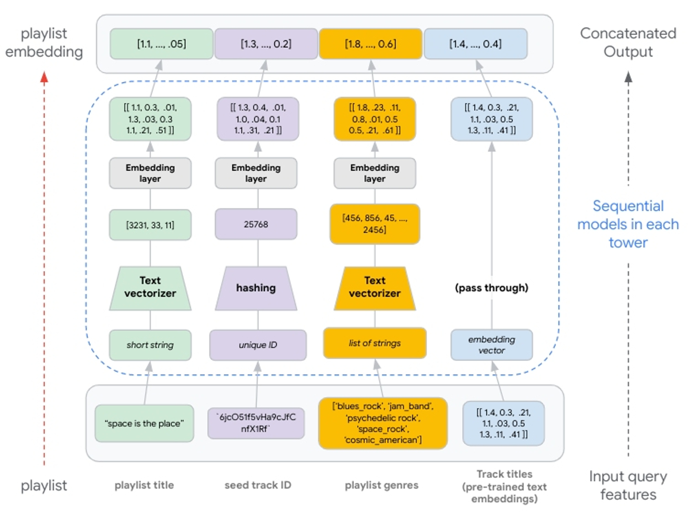
Figure 8: Illustration of feature processing from input to concatenated output. Text features are generated via n-grams. Integer indexes of n-grams are passed to an embedding layer. Hashing produces unique integers up to 1,000,000; values passed to an embedding layer. If using pre-trained embeddings, these are passed through the tower without transformation and concatenated with the other embedding representations.

Hashing vs StringLookup() layers

Hashing is generally recommended when fast performance is needed and is preferred over string lookups because it skips the need for a lookup table. Setting the proper bin size for the hashing layer is critical. When there are more unique values than hashing bins, values start getting placed into the same bins, and this can negatively impact our recommendations. This is commonly referred to as a hashing collision, and can be avoided when building the model by allocating enough bins for the unique values. See turning categorical features into embeddings for more details.

TextVectorization() layers

The key to text features is to understand if creating additional NLP features with the TextVectorization layer is helpful. If additional context derived from the text feature is minimal, it may not be worth the cost to model training. This layer needs to be adapted from the source dataset, meaning the layer requires a scan of the training data to create lookup dictionaries for the top N n-grams (set by max_tokens).

Decision tree to guide feature engineering strategy
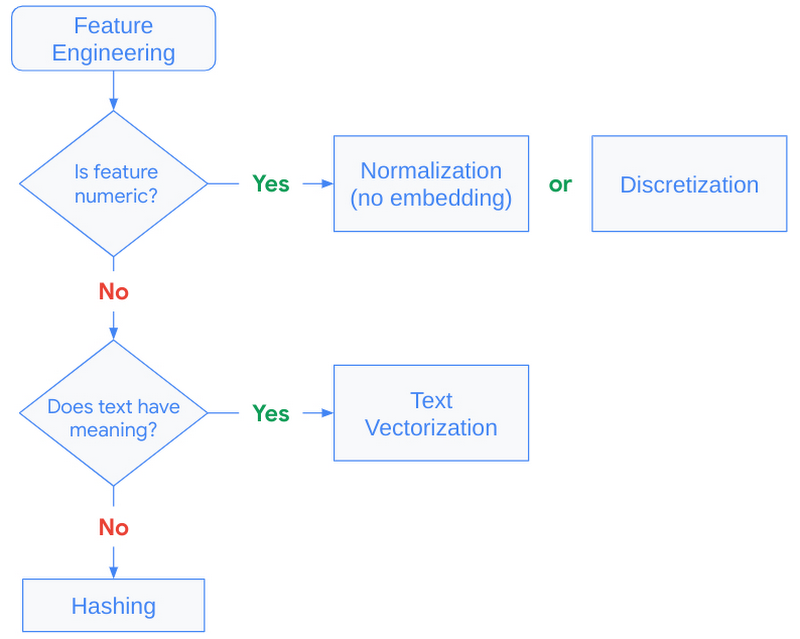
Figure 9: Decision tree to guide feature engineering strategy.

Efficient retrieval with Matching Engine

So far we’ve discussed how to map queries and candidates to the shared embedding space. Now let’s discuss how to best use this shared embedding space for efficient serving.

Recall at serving time, we will use the trained query tower to compute the embeddings for a query (playlist) and use this embedding vector in a nearest neighbor search for the most similar candidate (track) embeddings. And, because the candidate dataset can grow to millions or billions of vectors, this nearest neighbor search often becomes a computational bottleneck for low-latency inference.

Many state-of-the-art techniques address the computational bottleneck by compressing the candidate vectors such that ANN calculations can be performed in a fraction of the time needed for an exhaustive search. The novel compression algorithm proposed by Google Research modifies these techniques to also optimize for the nearest neighbor search accuracy. The details of their proposed technique are described here, but fundamentally their approach seeks to compress the candidate vectors such that the original distances between vectors are preserved. Compared to previous solutions, this results in a more accurate relative ranking of a vector and its nearest neighbors, i.e., it minimizes distorting the vector similarities our model learned from the training data.

Fully managed vector database and ANN service

Matching Engine is a managed solution utilizing these techniques for efficient vector similarity search. It offers customers a highly scalable vector database and ANN service while alleviating the operational overhead of developing and maintaining similar solutions, such as the open sourced ScaNN library. It includes several capabilities that simplify production deployments, including:

  • Large-scale: supports large embedding datasets with up to 1 billion embedding vectors
  • Incremental updates: depending on the number of vectors, complete index rebuilds can take hours. With incremental updates, customers can make small changes without building a new index (see Update and rebuild an active index for more details)
  • Dynamic rebuilds: when an index grows beyond its original configuration, Matching Engine periodically re-organizes the index and serving structure to ensure optimal performance
  • Autoscaling: underlying infrastructure is autoscaled to ensure consistent performance at scale
  • Filtering and diversity: ability to include multiple restrict and crowding tags per vector. At query inference time, use boolean predicates to filter and diversify retrieved candidates (see Filter vector matches for more details)

When creating an ANN index, Matching Engine uses the Tree-AH strategy to build a distributed implementation of our candidate index. It combines two algorithms:

  • Distributed search tree for hierarchically organizing the embedding space. Each level of this tree is a clustering of the nodes at the next level down, where the final leaf-level is a clustering of our candidate embedding vectors
  • Asymmetric hashing (AH) for fast dot product approximation algorithm used to score similarity between a query vector and the search tree nodes
Illustration showing the partitioned candidate vector dataset.
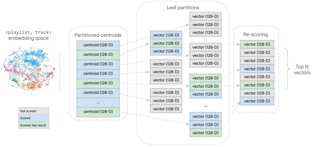
Figure 10: conceptual representation of the partitioned candidate vector dataset. During query inference, all partition centroids are scored. In the centroids most similar to the query vector, all candidate vectors are scored. The scored candidate vectors are aggregated and re-scored, returning the top N candidate vectors.

This strategy shards our embedding vectors into partitions, where each partition is represented by the centroid of the vectors it contains. The aggregate of these partition centroids form a smaller dataset summarizing the larger, distributed vector dataset. At inference time, Matching Engine scores all the partitioned centroids, then scores the vectors within the partitions whose centroids are most similar to the query vector.

Conclusion

In this blog we took a deep dive into understanding critical components of a candidate retrieval workflow using TensorFlow Recommenders and Vertex AI Matching Engine. We took a closer look at the foundational concepts of two-tower architectures, explored the semantics of query and candidate entities, and discussed how things like the structure of training examples can impact the success of candidate retrieval.

In a subsequent post we will demonstrate how to use Vertex AI and other Google Cloud services to implement these techniques at scale. We’ll show how to leverage BigQuery and Dataflow to structure training examples and convert them to TFRecords for model training. We’ll outline how to structure a Python application for training two-tower models with the Vertex AI Training service. And we’ll detail the steps for operationalizing the trained towers.

Read More

Serving With TF and GKE: Stable Diffusion

Serving With TF and GKE: Stable Diffusion

Posted by Chansung Park and Sayak Paul (ML and Cloud GDEs)

Generative AI models like Stable Diffusion1 that lets anyone generate high-quality images from natural language text prompts enable different use cases across different industries. These types of models allow people to generate these images not only from images but also condition them with other inputs such as segmentation maps, other images, depth maps, etc. In many ways, an end Stable Diffusion system (such as this) is often very complete. One gives a free-form text prompt to start the generation process, and in the end, an image (or any data in the continuous modality) gets generated.

In this post, we discuss how TensorFlow Serving (TF Serving) and Google Kubernetes Engine (GKE) can serve such a system with online deployment. Stable Diffusion is just one example of many such systems that TF and GKE can serve with online deployment. We start by breaking down Stable Diffusion into main components and how they influence the subsequent consideration for deployment. Then we dive deep into the deployment-specific bits such as TF Serving deployment and k8s cluster configuration. Our code is open-sourced in this repository.

Let’s dive in.

Stable Diffusion in a nutshell

Stable Diffusion, is comprised of three sub-models:

  • CLIP’s text tower as the Text Encoder,
  • Diffusion Model (UNet), and
  • Decoder of a Variational Autoencoder

When generating images from an input text prompt, the prompt is first embedded into a latent space with the text encoder. Then an initial noise is sampled, which is fed to the Diffusion model along with the text embeddings. This noise is then denoised using the Diffusion model in a continuous manner – the so-called “diffusion” process. The output of this step is a denoise latent, and it is fed to the Decoder for final image generation. Figure 1 provides an overview.

(For a more complete overview of Stable Diffusion, refer to this post.)

Flow chart illustrating stable diffusion architecture
Figure 1. Stable Diffusion Architecture

As mentioned above, three sub-models of Stable Diffusion work in a sequential manner. It’s common to run all three models on a single server (which constructs the end Stable Diffusion system) and serve the system as a whole.

However, because each component is a standalone deep learning model, each one could be served independently. This is particularly useful because each component has different hardware requirements. This can also have potentially improved resource utilization. The text encoder can still be run on moderate CPUs, whereas the other two should be run on GPUs, especially the UNet should be served with larger size GPUs (~3.4 GBs in size).

Flow chart illustrating decomposing stable diffusion in three parts
Figure 2. Decomposing Stable Diffusion in three parts

Figure 2 shows the Stable Diffusion serving architecture that packages each component into a separate container with TensorFlow Serving, which runs on the GKE cluster. This separation brings more control when we think about local compute power and the nature of fine-tuning of Stable Diffusion as shown in Figure 3.

NOTE: TensorFlow Serving is a flexible, high-performance serving system for machine learning models, designed for production environments, which is widely adopted in industry. The benefits of using it include GPU serving support, dynamic batching, model versioning, RESTful and gRPC APIs, to name but a few.

In modern personal devices such as desktops and mobile phones, it is common that they are equipped with moderate CPUs and sometimes GPU/NPUs. In this case, we could selectively run the UNet and/or Decoder in the cloud using high capacity GPUs while running the text encoder locally on the user’s device. In general, this approach allows us to flexibly architect the Stable Diffusion system in a way to maximize the resource utilization.

Flow chart illustrating flexible serving structure of stable diffusion
Figure 3. Flexible serving structure of Stable Diffusion

One more scenario to consider is fine-tuned Stable Diffusion. Many variations such as DreamBooth, Textual Inversion, or style transfer have shown that modifying only one or two components (usually Text Encoder and UNet) can generate images with new concepts or different styles. In this case, we could selectively deploy more of certain fine-tuned models on separate instances or replace existing models without touching other parts.

Wrapping Stable Diffusion in SavedModels

In order to serve a TensorFlow/Keras model with TF Serving, it should be saved in the SavedModel format. After that, the model can be served by TF Serving, a high-performance serving system for machine learning models, specially designed for production environments. The potentially non-trivial parts of making a SavedModel could be divided into three parts:

  1. defining an appropriate input signature specification of the underlying model,
  2. performing computations with the underlying model so that everything can be compiled in native TensorFlow, and
  3. including most of the pre and post-processing operations within the SavedModel graph itself to reduce training/serving skew (this is optional, but highly recommended).

To make the Stable Diffusion class shipped in KerasCV compatible with TF Serving, we need to first isolate the sub-networks (as mentioned above) of the class. Recall that we have got three sub-networks here: text encoder, diffusion model, and a decoder. We then have to serialize these networks as SavedModels.

A diffusion system also involves iterative sampling where a noise vector is gradually turned into an image. KerasCV’s Stable Diffusion class implements the sampling process with non-TensorFlow operations. So, we need to eliminate those operations and ensure that it’s implemented in pure TensorFlow so that there is end-to-end compatibility. This was the single most challenging aspect for us in the whole project.

Since the serialization of the text encoder and the decoder is straightforward, we’ll skip that in this post and instead, focus on the serialization of the diffusion model, including the sampling process. You can find an end-to-end notebook here.

Diffusion Model and Iterative Sampling

We start by defining an input signature dictionary for the SavedModel to be serialized. In this case, the inputs consist:

  • context, that denotes embeddings of the input text prompt extracted with the text encoder
  • unconditional_context, that denotes the embeddings of a so-called “null prompt” (see classifier-free guidance)
  • num_steps, that denotes the number of sampling steps for the reverse diffusion process
  • batch_size, that denotes the number of images to be returned
from keras_cv.models.stable_diffusion.constants import ALPHAS_CUMPROD_TF
import tensorflow as tf

IMG_HEIGHT = 512
IMG_WIDTH = 512
MAX_PROMPT_LENGTH = 77
ALPHAS_CUMPROD_TF = tf.constant(ALPHAS_CUMPROD_TF)
UNCONDITIONAL_GUIDANCE_SCALE = 7.5
HIDDEN_DIM = 768
SEED = None

signature_dict = {
"context": tf.TensorSpec(shape=[None, MAX_PROMPT_LENGTH, HIDDEN_DIM], dtype=tf.float32, name="context"),
"unconditional_context": tf.TensorSpec(
shape=[None, MAX_PROMPT_LENGTH, HIDDEN_DIM], dtype=tf.float32, name="unconditional_context"
),
"num_steps": tf.TensorSpec(shape=[], dtype=tf.int32, name="num_steps"),
"batch_size": tf.TensorSpec(shape=[], dtype=tf.int32, name="batch_size"),
}

Next up, we implement the iterative reverse diffusion process that involves the pre-trained diffusion model. diffusion_model_exporter() takes this model as an argument. serving_fn() is the function we use for exporting the final SavedModel. Most of this code is taken from the original KerasCV implementation here, except it has got all the operations implemented in native TensorFlow.

def diffusion_model_exporter(model: tf.keras.Model):
@tf.function
def get_timestep_embedding(timestep, batch_size, dim=320, max_period=10000):
...
@tf.function(input_signature=[signature_dict])
def serving_fn(inputs):
img_height = tf.cast(tf.math.round(IMG_HEIGHT / 128) * 128, tf.int32)
img_width = tf.cast(tf.math.round(IMG_WIDTH / 128) * 128, tf.int32)

batch_size = inputs["batch_size"] num_steps = inputs["num_steps"]

context = inputs["context"] unconditional_context = inputs["unconditional_context"]

latent = tf.random.normal((batch_size, img_height // 8, img_width // 8, 4))

timesteps = tf.range(1, 1000, 1000 // num_steps)
alphas = tf.map_fn(lambda t: ALPHAS_CUMPROD_TF[t], timesteps, dtype=tf.float32)
alphas_prev = tf.concat([[1.0], alphas[:-1]], 0)

index = num_steps - 1
latent_prev = None
for timestep in timesteps[::-1]:
latent_prev = latent
t_emb = get_timestep_embedding(timestep, batch_size)
unconditional_latent = model(
[latent, t_emb, unconditional_context], training=False
)
latent = model([latent, t_emb, context], training=False)
latent = unconditional_latent + UNCONDITIONAL_GUIDANCE_SCALE * (
latent - unconditional_latent
)
a_t, a_prev = alphas[index], alphas_prev[index] pred_x0 = (latent_prev - tf.math.sqrt(1 - a_t) * latent) / tf.math.sqrt(a_t)
latent = (
latent * tf.math.sqrt(1.0 - a_prev) + tf.math.sqrt(a_prev) * pred_x0
)
index = index - 1

return {"latent": latent}

return serving_fn

Then, we can serialize the diffusion model as a SavedModel like so:

tf.saved_model.save(
diffusion_model,
path_to_serialize_the_model,
signatures={"serving_default": diffusion_model_exporter(diffusion_model)},
)

Here, diffusion_model is the pre-trained diffusion model initialized like so:

from keras_cv.models.stable_diffusion.diffusion_model import DiffusionModel
diffusion_model = DiffusionModel(IMG_HEIGHT, IMG_WIDTH, MAX_PROMPT_LENGTH)

Deploy Stable Diffusion to GKE

Once you have successfully created TensorFlow SavedModels, it is quite straightforward to deploy them with TensorFlow Serving to a GKE cluster in the following steps.

  1. Write Dockerfiles which are based on the TensorFlow Serving base image
  2. Create a GKE cluster with accelerators attached
  3. Apply NVIDIA GPU driver installation daemon to install the driver on each node
  4. Write deployment manifests with GPU allocation
  5. Write service manifests to expose the deployments
  6. Apply all the manifests

The easiest way to wrap a SavedModel in TensorFlow Serving is to leverage the pre-built TensorFlow Serving Docker images. Depending on the configuration of the machine that you’re deploying to, you should choose either tensorflow/serving:latest or tensorflow/serving:latest-gpu. Because all the steps besides GPU-specific configuration are the same, we will explain this section with an example of the Diffusion Model part only.

By default, TensorFlow Serving recognizes embedded models under /models, so the entire SavedModel folder tree should be placed inside /models/{model_name}/{version_num}. A single TensorFlow Serving instance can serve multiple versions of multiple models, so that is why we need such a {model_name}/{version_num} folder structure. A SavedModel can be exposed as an API by setting a special environment variable MODEL_NAME, which is used for TensorFlow Serving to look for which model to serve.

FROM tensorflow/serving:latest-gpu
...
RUN mkdir -p /models/text-encoder/1
RUN cp -r tfs-diffusion-model/* /models/diffusion-model/1/
ENV MODEL_NAME=diffusion-model
...

Next step is to create a GKE cluster. You can do this by using either Google Cloud Console or gcloud container CLI as below. If you want accelerators available on each node, you can specify how many of which GPUs to be attached with --accelerator=type={ACCEL_TYPE}, count={ACCEL_NUM} option.

$ gcloud container clusters create {CLUSTER_NAME}
--machine-type={MACHINE_TYPE} # n1-standard-4
--accelerator=type={GPU_TYPE},count={GPU_NUM} # nvidia-tesla-v100, 1
...

Once the cluster is successfully created, and if the nodes in the cluster have accelerators attached, an appropriate driver for them should be installed correctly. This is done by running a special DaemonSet, which tries to install the driver on each node. If the driver has not been successfully installed, and if you try to apply Deployment manifests requiring accelerators, the status of the pod remains as Pending.

$ DRIVER_URL = https://raw.githubusercontent.com/GoogleCloudPlatform/container-engine-accelerators/master/nvidia-driver-installer/cos/daemonset-preloaded.yaml

$
kubectl apply -f $DRIVER_URL

Make sure all the pods are up and running with kubectl get pods -A command. Then, we are ready to apply prepared Deployment manifests. Below is an example of the Deployment manifest for the Diffusion Model. The only consideration you need to take is to specify which resource the pods of the Deployment should consume. Because the Diffusion Model needs to be run on accelerators, resources:limits:nvidia.com/gpu: {ACCEL_NUM} should be set.

Furthermore, if you want to expose gRPC and RestAPI at the same time, you need to set containerPort for both. TensorFlow Serving exposes the two endpoints via 8500 and 8501, respectively, by default, so both ports should be specified.

apiVersion: apps/v1
kind: Deployment
...
spec:
containers:
- image: {IMAGE_URI}
...
args: ["--rest_api_timeout_in_ms=1200000"] ports:
- containerPort: 8500
name: grpc
- containerPort: 8501
name: restapi
resources:
limits:
nvidia.com/gpu: 1

One more thing to note is that --rest_api_timeout_in_ms flag is set in args with a huge number. It takes a long time for heavy models to run inference. Since the flag is set to 5,000ms by default which is 5 seconds, sometimes timeout occurs before the inference is done. You can experimentally find out the right number, but we simply set this with a high enough number to demonstrate this project smoothly.

The final step is to apply prepared manifest files to the provisioned GKE cluster. This could be easily done with the kubectl apply -f command. Also, you could apply Service and Ingress depending on your needs. Because we simply used vanilla LoadBalancer type of Service for demonstration purposes, it is not listed in this blog. You can find all the Dockerfiles, and the Deployment and Service manifests in the accompanying GitHub repository.

Let’s generate images!

Once all the TensorFlow Serving instances are deployed, we could generate images by calling their endpoints. We will show how to do it through RestAPI, but you could do the same with the gRPC channel as well. The image generation process could be done in the following steps:

  1. Prepare tokens for the prompt of your choice
  2. Send the tokens to the Text Encoder endpoint
  3. Send context and unconditional context obtained from the Text Encoder to the Diffusion Model endpoint
  4. Send latent obtained from the Diffusion Model to the Decoder endpoint
  5. Plot the generated images

Since it is non-trivial to embed a tokenizer into the Text Encoder itself, we need to prepare the tokens for the prompt of your choice. KerasCV library provides SimpleTokenizer in the keras_cv.models.stable_diffusion.clip_tokenizer module, so you could simply pass the prompt to it. Since the Diffusion Model is designed to accept 77 tokens, the tokens are padded with MAX_PROMPT_LENGTH up to 77 long.

NOTE: Since KerasCV comes with lots of modules that we don’t need for tokenization, it is not recommended to import the entire library. Instead, you could simply copy the codes for the SimpleTokenizer in your environment. Due to incompatibility issues, the current tokenizer cannot be shipped as a part of the Text Encoder SavedModel.

from keras_cv.models.stable_diffusion.clip_tokenizer import SimpleTokenizer

MAX_PROMPT_LENGTH = 77
PADDING_TOKEN = 49407

tokenizer = SimpleTokenizer()

prompt = "photograph of an astronaut riding a horse in a green desert"
tokens = tokenizer.encode(prompt)
tokens = tokens + [PADDING_TOKEN] * (MAX_PROMPT_LENGTH - len(tokens))

Once the tokens are prepared, we could simply pass it to the Diffusion Model’s endpoint. The headers and the way to call the all endpoints are identical as below, so we will omit it in the following steps. Just keep in mind you set the ADDRESS and the MODEL_NAME correctly, which is identical to the one we set in each Dockerfile.

import requests

ADDRESS = ENDPOINT_IP_ADDRESS

headers = {"content-type": "application/json"}
payload = ENDPOINT_SPECIFIC

response = requests.post(
f"http://{ADDRESS}:8501/v1/models/{MODEL_NAME}:predict",
data=payload, headers=headers
)

As you see, each payload is dependent on the upstream tasks. For instance, we pass tokens to the Text Encoder’s endpoint, context and unconditional_context retrieved from the Text Encoder to the Diffusion Model’s endpoint, and latent retrieved from the Diffusion Model to Decoder’s endpoint. The signature_name should be the same as when we created SavedModel with the signatures argument.

import json

BATCH_SIZE = 4

payload_to_text_encoder = json.dumps(
{
"signature_name": "serving_default",
"inputs": {
"tokens": tokens,
"batch_size": BATCH_SIZE
}
})

# json_response is from the text_encoder's response
# json_response = json.loads(response.text)
payload_to_diffusion_model = json.dumps(
{
"signature_name": "serving_default",
"inputs": {
"batch_size": BATCH_SIZE,
"context": json_response['outputs']['context'],
"num_steps": num_steps,
"unconditional_context": json_response['outputs']['unconditional_context'] }
})

# json_response is from the diffusion_model's response
# json_response = json.loads(response.text)
payload_to_decoder = json.dumps(
{
"signature_name": "serving_default",
"inputs": {
"latent": json_response['outputs'],
}
})

The final response from the Decoder’s endpoint contains a full of pixel values in a list, so we need to convert those into a format that the environment of your choice could understand as images. For demonstration purposes, we used the tf.convert_to_tensor() utility function that turns the Python list into TensorFlow’s Tensor. However, you could plot the images in different languages, too, with your most familiar methods.

import matplotlib.pyplot as plt

def plot_images(images):
plt.figure(figsize=(20, 20))
for i in range(len(images)):
ax = plt.subplot(1, len(images), i + 1)
plt.imshow(images[i])
plt.axis("off")

plot_images(
tf.convert_to_tensor(json_response['outputs']).numpy()
)

Four AI generated images of an astronaut riding a horse
Figure 4. Generated images with three TensorFlow Serving endpoints

Note on XLA compilation

We can obtain a speed-up of 17 – 25% by incorporating compiling the SavedModels to be XLA compatible. Note that the individual sub-networks of the Stable Diffusion class are fully XLA compatible. But in our case, the SavedModels also contain important operations that are in native TensorFlow, such as the reverse diffusion process.

For deployment purposes, this speed-up could be impactful. To know more, check out the following repository: https://github.com/sayakpaul/xla-benchmark-sd.

Conclusion

In this blog post, we explored what Stable Diffusion is, how it could be decomposed into the Text Encoder, Diffusion Model, and Decoder, and why it might be beneficial for better resource utilization. Also, we touched upon the concrete demonstration about the deployment of the decomposed Stable Diffusion by creating SavedModels, containerizing them in TensorFlow Serving, deploying them on the GKE cluster, and running image generations. We used the vanilla Stable Diffusion, but feel free to try out replacing the only Diffusion Model with in-painting or pokemon fine-tuned diffusion models.

References

CLIP: Connecting text and images, OpenAI, https://openai.com/research/clip.

The Illustrated Stable Diffusion, Jay Alammar, https://jalammar.github.io/illustrated-stable-diffusion/.

Stable Diffusion, Stability AI, https://stability.ai/stable-diffusion.

Acknowledgements

We are grateful to the ML Developer Programs team that provided Google Cloud credits to support our experiments. We thank Robert Crowe for providing us with helpful feedback and guidance.

___________

1 Stable Diffusion is not owned or operated by Google. It is made available by Stability AI. Please see their site for more information: https://stability.ai/blog/stable-diffusion-public-release.Read More

Get ready for Google I/O

Get ready for Google I/O

Posted by Timothy Jordan, Director, Developer Relations & Open Source

I/O is just a few days away and we couldn’t be more excited to share the latest updates across Google’s developer products, solutions, and technologies. From keynotes to technical sessions and hands-on workshops, these announcements aim to help you build smarter and ship faster.

Here are some helpful tips to maximize your experience online.

Start building your personal I/O agenda

Starting now, you can save the Google and developer keynotes to your calendar and explore the program to preview content. Here are just a few noteworthy examples of what you’ll find this year:

What’s new in Android

Get the latest news in Android development: Android 14, form factors, Jetpack + Compose libraries, Android Studio, and performance.

What’s new in Web

Explore new features and APIs that became stable across browsers on the Web Platform this year.

What’s new in Generative AI

Discover a new suite of tools that make it easy for developers to leverage and build on top of Google’s large language models.

What’s new in Google Cloud

Learn how Google Cloud and generative AI will help you develop faster and more efficiently.

For the best experience, create or connect a developer profile and start saving content to My I/O to build your personal agenda. With over 200 sessions and other learning material, there’s a lot to cover, so we hope this will help you get organized.

This year we’ve introduced development focus filters to help you navigate content faster across mobile, web, AI, and cloud technologies. You can also peruse content by topic, type, or experience level so you can find what you’re interested in, faster.

Connect with the community

After the keynotes, you can talk to Google experts and other developers online in I/O Adventure chat. Here you can ask questions about new releases and learn best practices from the global developer community.

If you’re craving community now, visit the Community page to meet people with similar interests in your area or find a watch party to attend.

We hope these updates are useful, and we can’t wait to connect online in May!

Read More

Training a recommendation model with dynamic embeddings

Training a recommendation model with dynamic embeddings

Posted by Thushan Ganegedara (GDE), Haidong Rong (Nvidia), Wei Wei (Google)

Modern recommenders heavily leverage embeddings to create vector representations of each user and candidate item. These embedding can then be used to calculate the similarity between users and items, so that users are recommended candidate items that are more interesting and relevant. But when working with data at scale, particularly in an online machine learning setting, embedding tables can grow in size dramatically, accumulating millions (and sometimes billions) of items. At this scale, it becomes impossible to store these embedding tables in memory. Furthermore, a large portion of the items might be rarely seen, so it does not make sense to keep dedicated embeddings for such rarely occurring items. A better solution would be to represent those items with one common embedding. This can dramatically reduce the size of the embedding table at a very small fraction of the performance cost. This is the main motivation behind dynamic embedding tables.

TensorFlow’s built-in tf.keras.layers.Embedding layer has a fixed size at creation time, so we need another approach. Fortunately, there is a TensorFlow SIG project exactly for this purpose: TensorFlow Recommenders Addons (TFRA). You can learn more from its repository, but at a high level TFRA leverages dynamic embedding technology to dynamically change embedding size and achieve better recommendation results than static embeddings. TFRA is fully TF2.0-compatible and works smoothly with the familiar Keras API interfaces, so it can be easily integrated with other TensorFlow products, such as TensorFlow Recommenders (TFRS).

In this tutorial we will build a movie recommender model by leveraging both TFRS and TFRA. We will use the MovieLens dataset, which contains anonymized data showing ratings given to movies by users. Our primary focus is to show how the dynamic embeddings provided in the TensorFlow Recommenders Addons library can be used to dynamically grow and shrink the size of the embedding tables in the recommendation setting. You can find the full implementation here and a walkthrough here.

Processing the data

Let’s first build a baseline model with TensorFlow Recommenders. We will follow the pattern of this TFRS retrieval tutorial to build a two-tower retrieval model. The user tower will take the user ID as the input, but the item tower will use the tokenized movie title as the input.

To handle the movie titles, we define a helper function that converts the movie titles to lowercase, removes any punctuation in a given movie title, and splits using spaces to generate a list of tokens. Finally we take only the up to max_token_length tokens (from the start) from the movie title. If a movie title has fewer tokens, all the tokens will be taken. This number is chosen based on some analysis and represents the 90th percentile in the title lengths in the dataset.

max_token_length = 6
pad_token = "[PAD]"
punctuation_regex = "[!"#$%&()*+,-./:;<=>?@[]\^_`{|}~\t\n]"

#First we’ll define a helper function that will process the movie titles for us.

def process_text(x: tf.Tensor, max_token_length: int, punctuation_regex: str) -> tf.Tensor:

return tf.strings.split(
tf.strings.regex_replace(
tf.strings.lower(x["movie_title"]), punctuation_regex, ""
)
)[:max_token_length]

We also pad the tokenized movie titles to a fixed length and split the dataset using the same random seed so that we get consistent validation results across training epochs. You can find detailed code in the ‘Processing datasets’ section of the notebook.

Building the two tower model

Our user tower is pretty much the same as in the TFRS retrieval tutorial (except it’s deeper), but for the movie tower there is a GlobalAveragePooling1D layer after the embedding lookup, which averages the embedding of movie title tokens to a single embedding.

def get_movie_title_lookup_layer(dataset: tf.data.Dataset) -> tf.keras.layers.Layer:
movie_title_lookup_layer = tf.keras.layers.StringLookup(mask_token=pad_token)
movie_title_lookup_layer.adapt(dataset.map(lambda x: x["movie_title"]))
return movie_title_lookup_layer

def build_item_model(movie_title_lookup_layer: tf.keras.layers.StringLookup):
vocab_size = movie_title_lookup_layer.vocabulary_size()
return tf.keras.models.Sequential([
tf.keras.layers.InputLayer(input_shape=(max_token_length), dtype=tf.string),
movie_title_lookup_layer,
tf.keras.layers.Embedding(vocab_size, 64),
tf.keras.layers.GlobalAveragePooling1D(),
tf.keras.layers.Dense(64, activation="gelu"),
tf.keras.layers.Dense(32),
tf.keras.layers.Lambda(lambda x: tf.math.l2_normalize(x, axis=1))
])

Next we are going to train the model.

Training the model

Training the model is simply calling fit() on the model with the required arguments. We will be using our validation dataset validation_ds to measure the performance of our model.

history = model.fit(datasets.training_datasets.train_ds, epochs=3, validation_data=datasets.training_datasets.validation_ds)

At the end, the output looks like below:

Epoch 3/3
220/220 [==============================] - 146s 633ms/step
......
val_factorized_top_k/top_10_categorical_accuracy: 0.0179 - val_factorized_top_k/top_50_categorical_accuracy: 0.0766 - val_factorized_top_k/top_100_categorical_accuracy: 0.1338 - val_loss: 12359.0557 - val_regularization_loss: 0.0000e+00 - val_total_loss: 12359.0557

We have achieved a top 100 categorical accuracy of 13.38% on the validation dataset.

Building the model with dynamic embeddings

Overview

We will now learn how we can use the dynamic embedding in the TensorFlow Recommenders Addons (TFRA) library, rather than a static embedding table. As the name suggests, as opposed to creating embeddings for all the items in the vocabulary up front, dynamic embedding would only grow the size of the embedding table on demand. This behavior really shines when dealing with millions and billions of items and users as some companies do. For these companies, it’s not surprising to find static embedding tables that would not fit in memory. Static embedding tables can grow up to hundreds of Gigabytes or even Terabytes, incapacitating even the highest memory instances available in cloud environments.

When you have an embedding table with large cardinality, the accessing weights will be quite sparse. Therefore, a hash-table based data structure is used to hold the weights and required weights for each iteration are retrieved from the underlying table structure. Here, to focus on the core functionality of the library, we will focus on a non-distributed setting. In this case, TFRA will choose cuckoo hashtable by default. But there are other solutions such as Redis, nvhash available.

A chart showing the various embedding solutions across distruted and non-distributed settings in the TFRA library

When using the dynamic embedding, we initialize the table with some initial capacity and the table will grow in size on demand as it sees more IDs during model training. For more information about motivation and inner mechanics, please refer to the RFC.

Types of embedding

Currently in the TFRA dynamic_embedding module, there are three types of embedding available:

  • Embedding – The most basic form of embeddings. This expects a 1D ([batch_size]) or 2D ([batch_size, time_steps]) tensor of IDs and outputs a [batch_size, embedding_dim] or [batch_size, time_steps, embedding_dim] sized tensor respectively.
  • SquashedEmbedding – This layer squashes the time step dimension based on some reduction operation (e.g. mean/sum) to transform a [batch_size, time_steps] sized tensor of IDs to a [batch_size, embedding_dim] tensor.
  • FieldwiseEmbedding – This type can handle multiple features (i.e. fields) at once. The layer takes n_slots as an argument and IDs are mapped to a slot within the layer. The layer would return a tensor of size [batch_size, n_slots, embedding_dim].

Defining the embedding layers

We will be using the Embedding to represent the user IDs and SquashedEmbedding to represent token IDs. Remember that each movie title has multiple tokens, therefore, we need a way to reduce the resulting token embeddings to a single representative embedding.

Note: The behavior of Embedding has changed from version 0.5 to 0.6. Please make sure to use version 0.6 for this tutorial.

With that, we can define the two towers as we did in the standard model. However, this time we’ll be using the dynamic embedding layers instead of static embedding layers.

def build_de_user_model(user_id_lookup_layer: tf.keras.layers.StringLookup) -> tf.keras.layers.Layer:
vocab_size = user_id_lookup_layer.vocabulary_size()
return tf.keras.Sequential([
tf.keras.layers.InputLayer(input_shape=(), dtype=tf.string),
user_id_lookup_layer,
de.keras.layers.Embedding(
embedding_size=64,
initializer=tf.random_uniform_initializer(),
init_capacity=int(vocab_size*0.8),
restrict_policy=de.FrequencyRestrictPolicy,
name="UserDynamicEmbeddingLayer"
),
tf.keras.layers.Dense(64, activation="gelu"),
tf.keras.layers.Dense(32),
tf.keras.layers.Lambda(lambda x: tf.math.l2_normalize(x, axis=1))
], name='user_model')

def build_de_item_model(movie_title_lookup_layer: tf.keras.layers.StringLookup) -> tf.keras.layers.Layer:
vocab_size = movie_title_lookup_layer.vocabulary_size()
return tf.keras.models.Sequential([
tf.keras.layers.InputLayer(input_shape=(max_token_length), dtype=tf.string),
movie_title_lookup_layer,
de.keras.layers.SquashedEmbedding(
embedding_size=64,
initializer=tf.random_uniform_initializer(),
init_capacity=int(vocab_size*0.8),
restrict_policy=de.FrequencyRestrictPolicy,
combiner="mean",
name="ItemDynamicEmbeddingLayer"
),
tf.keras.layers.Dense(64, activation="gelu"),
tf.keras.layers.Dense(32),
tf.keras.layers.Lambda(lambda x: tf.math.l2_normalize(x, axis=1))
])

With the user tower and movie tower models defined, we can define the retrieval model as usual.

Creating and compiling the final model

As a final step in model building, we’ll create the model and compile it.

def create_de_two_tower_model(dataset: tf.data.Dataset, candidate_dataset: tf.data.Dataset) -> tf.keras.Model:

user_id_lookup_layer = get_user_id_lookup_layer(dataset)
movie_title_lookup_layer = get_movie_title_lookup_layer(dataset)
user_model = build_de_user_model(user_id_lookup_layer)
item_model = build_de_item_model(movie_title_lookup_layer)
task = tfrs.tasks.Retrieval(
metrics=tfrs.metrics.FactorizedTopK(
candidate_dataset.map(item_model)
),
)

model = DynamicEmbeddingTwoTowerModel(user_model, item_model, task)
optimizer = de.DynamicEmbeddingOptimizer(tf.keras.optimizers.Adam())
model.compile(optimizer=optimizer)

return model

datasets = create_datasets()
de_model = create_de_two_tower_model(datasets.training_datasets.train_ds, datasets.candidate_dataset)

Note the usage of the DynamicEmbeddingOptimizer wrapper around the standard TensorFlow optimizer. It is mandatory to wrap the standard optimizer in a DynamicEmbeddingOpitmizer as it will provide specialized functionality needed to train the weights stored in a hashtable. We can now train our model.

Training the model

Training the model is quite straightforward, but will involve a bit more extra effort as we’d like to log some extra information. We will perform the logging through a tf.keras.callbacks.Callback object. We’ll name this DynamicEmbeddingCallback.

epochs = 3
history_de = {}
history_de_size = {}
de_callback = DynamicEmbeddingCallback(de_model, steps_per_logging=20)

for epoch in range(epochs):

datasets = create_datasets()
train_steps = len(datasets.training_datasets.train_ds)

hist = de_model.fit(
datasets.training_datasets.train_ds,
epochs=1,
validation_data=datasets.training_datasets.validation_ds,
callbacks=[de_callback] )

for k,v in de_model.dynamic_embedding_history.items():
if k=="step":
v = [vv+(epoch*train_steps) for vv in v] history_de_size.setdefault(k, []).extend(v)

for k,v in hist.history.items():
history_de.setdefault(k, []).extend(v)

We have taken the loop that goes through the epochs out of the fit() function. Then in every epoch we re-create the dataset, as that will provide a different shuffling of the training dataset. We will train the model for a single epoch within the loop. Finally we accumulate the logged embedding sizes in history_de_size (this is provided by our custom callback) and performance metrics in history_de.

The callback is implemented as follows.

class DynamicEmbeddingCallback(tf.keras.callbacks.Callback):

def __init__(self, model, steps_per_logging, steps_per_restrict=None, restrict=False):
self.model = model
self.steps_per_logging = steps_per_logging
self.steps_per_restrict = steps_per_restrict
self.restrict = restrict

def on_train_begin(self, logs=None):
self.model.dynamic_embedding_history = {}

def on_train_batch_end(self, batch, logs=None):

if self.restrict and self.steps_per_restrict and (batch+1) % self.steps_per_restrict == 0:

[
self.model.embedding_layers[k].params.restrict(
num_reserved=int(self.model.lookup_vocab_sizes[k]*0.8),
trigger=self.model.lookup_vocab_sizes[k]-2 # UNK & PAD tokens
) for k in self.model.embedding_layers.keys()
]

if (batch+1) % self.steps_per_logging == 0:

embedding_size_dict = {
k:self.model.embedding_layers[k].params.size().numpy()
for k in self.model.embedding_layers.keys()
}

for k, v in embedding_size_dict.items():
self.model.dynamic_embedding_history.setdefault(f"embedding_size_{k}", []).append(v)
self.model.dynamic_embedding_history.setdefault(f"step", []).append(batch+1)

The callback does two things:

  • Logs the sizes of the embedding layers every steps_per_logging iterations
  • Reduces the size of the embedding table to an 80% size of the total vocabulary size if restrict=True(This is set to False by default)

Let’s understand what reducing the size means and why it is important.

Reducing the size of the embedding table

An important topic we still haven’t discussed is how to reduce the size of the embedding table, should it grow over some predefined threshold. This is a powerful functionality as it allows us to define a threshold over which the embedding table should not grow. This will allow us to work with large vocabularies while keeping the memory requirement under the memory limitations we may have. We achieve this by calling restrict() on the underlying variables of the embedding layer as shown in the DynamicEmbeddingCallback. restrict() takes two arguments in: num_reserved (the size after the reduction) and trigger (size at which the reduction should be triggered). The policy that governs how the reduction is performed is defined using the restrict_policy argument in the layer construct. You can see that we are using the FrequencyRestrictPolicy. This means the least frequent items will be removed from the embedding table. The callback enables a user to set how frequently the reduction should get triggered by setting the steps_per_restrict and restrict arguments in the DynamicEmbeddingCallback.

Reducing the size of the embedding table makes more sense when you have streaming data. Think about an online learning setting, where you are training the model every day (or even every hour) on some incoming data. You can think of the outer for loop (i.e. epochs) representing days. Each day you receive a dataset (containing user interactions from the previous day for example) and you train the model from the previous checkpoint. In this case, you can use the DynamicEmbeddingCallback to trigger a restrict if the embedding table grows over the size defined in the trigger argument.

Analyzing performance

Here we analyze the performance of three variants.

  • The standard retrieval model (which uses a static embedding table)
  • Retrieval model using dynamic embedding but no restrict performed
  • Retrieval model using dynamic embedding with restrict performed
A graph showing Model accuracy with and without dynamic embeddings

You can see that the model using dynamic embeddings (solid green line) has comparative validation performance to the baseline (solid red line). You can see a similar trend in the training accuracy as well. In practice, dynamic embeddings can often be seen to improve accuracy in a large-scale online learning setup.

Finally, we can see that restrict has a somewhat detrimental effect on the validation accuracy, which is understandable. Since we’re working with a relatively small dataset with a small number of items, the reduction could be getting rid of embeddings that are best kept in the table. For example, you can increase the num_reserved argument (e.g. set it to int(self.model.lookup_vocab_sizes[k]*0.95)) in the restrict function which would yield performance that improves towards the performance of without restrict.

Next we look at how dynamic the embedding tables really are over time.

A graph showing changes in the embedding size over time

We can see that when restrict is not used, the embedding table grows to the full size of the vocabulary (dashed line) and stays there. However when restrict is triggered (dotted line), the size drops and grows in size again as it encounters new IDs.

It is also important to note that constructing a proper validation is not a trivial task. There are considerations such as out-of-sample validation, out-of-time validation, stratification, etc. that needs to be taken into account carefully. However for this exercise, we have not focused on such factors and created a validation set by sampling randomly from the existing dataset.

Conclusion

Using dynamic embedding tables is a powerful way to perform representation learning when working with large sets of items containing millions or billions of entities. In this tutorial, we learnt how to use the dynamic_embedding module provided in the TensorFlow Recommender Addons library to achieve this. We first explored the data and constructed tf.data.Dataset objects by extracting the features we’ll be using for our model training and evaluation. Next we defined a model that uses static embedding tables to use as an evaluation baseline. We then created a model that uses dynamic embedding and trained it on the data. We saw that using dynamic embeddings, the embedding tables grow only on demand and still achieve comparable performance with the baseline. We also discussed how the restrict functionality can be used to shrink the embedding table if it grows past a pre-defined threshold.

We hope this tutorial gives you a good conceptual introduction to TFRA and dynamic embeddings, and helps you think about how you can leverage it to enhance your own recommenders. If you would like to have a more in-depth discussion, please visit the TFRA repository.

Read More

Counterfactual Logit Pairing

Counterfactual Logit Pairing

Posted by Bhaktipriya Radharapu, Software Engineer

TensorFlow Model Remediation is an open source toolkit that showcases solutions to help mitigate unfair bias in Machine Learning models. The toolkit offers resources to build fairer models for everyone – in line with Google’s AI Principles. Today, we’re excited to announce a new technique within the TensorFlow Model Remediation Library called Counterfactual Logit Pairing (CLP) to address unintended bias in ML models.

ML models are prone to making incorrect predictions when a sensitive attribute in an input is removed or replaced, leading to unintended bias. For instance, the Perspective API, used to identify offensive or toxic text in comments, revealed a positive correlation between identity terms referencing race or sexual orientation and the predicted toxicity score. For instance, the phrase “I am a lesbian” received a toxicity score of 0.51, while “I am a man” received a lower toxicity score of 0.2. This correlation resulted in higher toxicity scores for some identity terms, even when used non-pejoratively. For more information on the Perspective API, see the blog post on unintended bias and identity terms.

Counterfactual Logit Pairing (CLP) is a technique that addresses such issues to ensure that a model’s prediction doesn’t change when a sensitive attribute referenced in an example is either removed or replaced. It improves a model’s robustness to such perturbations, and can positively influence a model’s stability, fairness, and safety.

CLP mitigates such counterfactual fairness issues at training time. It does so by adding an additional loss to the model’s training loss, which penalizes the difference in the model’s outputs between training examples and their counterfactuals.

Another advantage of using CLP is that you can use this even on unlabelled data. As long as the model treats the counterfactual examples similarly you can validate that your model is adhering to counterfactual fairness.

For an in-depth discussion on this topic, see research on counterfactual fairness, adversarial logit pairing, and counterfactual logit pairing.

Counterfactual Logit Pairing Walkthrough:

The CLP with Keras codelab provides an end-to-end example. In this overview, we’ll emphasize key points from the notebook, while providing additional context.

The notebook trains a text classifier to identify toxic content. This type of model attempts to identify content that is rude, disrespectful or otherwise likely to make someone leave a discussion, and assigns the content a toxicity score. For this task, our baseline model will be a simple Keras sequential model pre-trained on the Civil Comments dataset.

We will use CLP to avoid having identity terms unfairly skew what is classified as offensive. We consider a narrow class of counterfactuals that involves removing gender and sexual orientation related identity tokens in the input, such as removing “gay” in the input “I’m a gay person” to create the counterfactual example “I’m a person.”

The high-level steps will be to:

  1. Calculate flip rate and flip count of the classifier on original and counterfactual examples.
  2. Build a counterfactual dataset using CounterfactualPackedInputs by performing a naive ablation based on term matching.
  3. Improve performance on flip rate and flip count by training with CLP.
  4. Evaluate the new model’s performance on flip rate and flip count.

Be aware that this is a minimal workflow to demonstrate usage of the CLP technique, and not a complete approach to fairness in machine learning. CLP addresses one specific challenge that may impact fairness in machine learning. See the Responsible AI toolkit for additional information on responsible AI and tools that can be used to complement CLP.

In a production setting, you would want to approach each of these steps with more rigor. For example:

  • Consider the fairness goals of your model. What qualifies as “fair” for your model? Which definitions of fairness are you trying to achieve?
  • Consider when counterfactual pairs should have the same prediction. Many syntactic counterfactuals generated by token substitution may not require identical output. Consider the application space and the potential societal impact of your model and understand when the outputs should be the same and when they shouldn’t be.
  • Consider using semantically and grammatically grounded counterfactuals instead of heuristic based ablations.
  • Experiment with the configuration of CLP by tuning hyperparameters to get optimal performance.

Let’s begin by examining the flip count and flip rate of the original model on the counterfactual examples. The flip count measures the number of times the classifier gives a different decision if the identity term in a given example is changed. The flip rate measures the total number of times that the classifier incorrectly provides an incorrect decision over the total count.

Let’s use the “Fairness Indicators widget” in the notebook to measure the flip rate and counts. Select flip_rate/overall in the widget. Notice that the overall flip rate for females is about 13% and male is about 14%, which are both higher than the overall dataset of 8%. This means that the model is likely to change the classification based on the presence of gender related terms.

We’ll now use CLP to try to reduce the model’s flip rate and flip count for gender-related terms in our dataset. We start by creating an instance of CounterfactualPackedInputs, which packs the original_input and counterfactual_data.

CounterfactualPackedInputs(
original_input=(x, y, sample_weight),
counterfactual_data:(original_x, counterfactual_x,
counterfactual_sample_weight)
)

We next remove instances of gender specific terms using the helper function, build_counterfactual_data. Note that we only include non-pejorative terms, as pejorative terms should have a different toxicity score. Requiring equal predictions across examples with pejorative terms would both weaken the model’s ability to perform its task and potentially increase harm to vulnerable groups.


sensitive_terms_to_remove = [
'aunt', 'boy', 'brother', 'dad', 'daughter', 'father', 'female', 'gay',
'girl', 'grandma', 'grandpa', 'grandson', 'grannie', 'granny', 'he',
'heir', 'her', 'him', 'his', 'hubbies', 'hubby', 'husband', 'king',
'knight', 'lad', 'ladies', 'lady', 'lesbian', 'lord', 'man', 'male',
'mom', 'mother', 'mum', 'nephew', 'niece', 'prince', 'princess',
'queen', 'queens', 'she', 'sister', 'son', 'uncle', 'waiter',
'waitress', 'wife', 'wives', 'woman', 'women'
]

# Convert the Pandas DataFrame to a TF Dataset
dataset_train_main = tf.data.Dataset.from_tensor_slices(
(data_train[TEXT_FEATURE].values, labels_train)).batch(BATCH_SIZE)

counterfactual_data = counterfactual.keras.utils.build_counterfactual_dataset(
original_dataset=dataset_train_main,
sensitive_terms_to_remove=sensitive_terms_to_remove)

counterfactual_packed_input = counterfactual.keras.utils.pack_counterfactual_data(
dataset_train_main,
counterfactual_data)

To train with a Counterfactual model, simply take the original model and wrap it in a CounterfactualModel with a corresponding loss and loss_weight. This will co-train the model on the main classification task and on the debiasing task using the CLP loss.

We are using 1.0 as the default loss_weight, but this is a parameter that can be tuned for your use case, since it depends on your model and product requirements. You should experiment with changing the value to see how it impacts the model, noting that increasing it would cause the model to penalize the counterfactual examples more heavily. You can test a range of values to explore the trade off between the task performance and the flip rate.

Here, we use the Pairwise Mean Squared Error Loss. You can try experimenting with other metrics in the suite to know which options offer the best results.

counterfactual_weight = 1.0

counterfactual_model = counterfactual.keras.CounterfactualModel(
baseline_model,
loss=counterfactual.losses.PairwiseMSELoss(),
loss_weight=counterfactual_weight)

# Compile the model normally after wrapping the original model.
# Note that this means we use the baseline's model's loss here.
optimizer = tf.keras.optimizers.Adam(learning_rate=0.001)
loss = tf.keras.losses.BinaryCrossentropy()
counterfactual_model.compile(optimizer=optimizer, loss=loss,
metrics=['accuracy'])

counterfactual_model.fit(counterfactual_packed_input,
epochs=1)

Once again, we evaluate the results by looking at the flip count and flip rate. Select “flip_rate/overall” within Fairness Indicators and compare the results for female and male between the two models. You should notice that the flip rate for overall, female, and male have all decreased by about 90%, which leaves the final flip rate for female at approximately 1.3% and male at approximately 1.4%.

You can get started with Counterfactual by visiting TensorFlow Responsible AI and learn more about evaluation fairness with Fairness Indicators.

Acknowledgements

The Counterfactual framework was developed in collaboration with
  • Amy Wang, Ben Packer, Bhaktipriya Radharapu, Christina Greer, Nick Blumm, Parker Barnes, Piyush Kumar, Sean O’Keefe, Shivam Jindal, Shivani Poddar, Summer Misherghi, Thomas Greenspan.
This research effort was jointly led by
  • Alex Beutel, Jilin Chen, Tulsee Doshi in collaboration with Sahaj Garg, Vincent Perot, Nicole Limtiaco, Ankur Taly, Ed H. Chi.
Further, this work was pursued in collaboration with
  • Andrew Smart, Francois Chollet, Molly FitzMorris, Tomer Kaftan, Mark Daoust, Daniel ‘Wolff’ Dobson, Soo Sung.

Read More

Celebrating Google Summer of Code Responsible AI Projects

Celebrating Google Summer of Code Responsible AI Projects

Posted by Bhaktipriya Radharapu, Software Engineer, Google Research

One of the key goals of Responsible AI is to develop software ethically and in a way that is responsive to the needs of society and takes into account the diverse viewpoints of users. Open source software helps address this by providing a way for a wide range of stakeholders to contribute.

To continue making Responsible AI development more inclusive and transparent, and in line with our AI Principles, Google’s Responsible AI team partnered with Google Summer of Code (GSoC), to provide students and professionals with the opportunity to contribute to open source projects that promote Responsible AI resources and practices. GSoC is a global, online program focused on bringing new contributors into open source software development. GSoC contributors work with an open source organization on a 12+ week programming project under the guidance of mentors. By bringing in new contributors and ideas, we saw that GSoC helped to foster a more innovative and creative environment for Responsible AI development.

This was also the first time several of Google’s Responsible AI tools, such as The Learning Interpretability Tool (LIT), TensorFlow Model Remediation and Data Cards Playbook, pulled in contributions from third-party developers across the globe, bringing in diverse and new developers to join us in our journey for building Responsible AI for all.

We’re happy to share the work completed by GSoC participants and share what they learned about working with state-of-the-art fairness and interpretability techniques, what we learned as mentors, and how rewarding summer of code was for each of us, and for the Responsible AI community.

We had the opportunity to mentor four developers – Aryan Chaurasia, Taylor Lee, Anjishnu Mukherjee, Chris Schmitz. Aryan successfully implemented XAI tutorials for LIT under the mentorship of Ryan Mullins, software engineer at Google. These showcase how LIT can be used to evaluate the performance of (multi-lingual) question-answering models, and understand behavioral patterns in text-to-image generation models.

Anjishnu implemented Tutorials for LIT also under the mentorship of Ryan Mullins. Anjishnu’s work influenced in-review research assessing professionals’ interpretability practices in production settings.

Chris, under the technical guidance of Jenny Hamer, a software engineer at Google, created two tutorials for TensorFlow Model Remediations’ experimental technique, Fair Data Reweighting. The tutorials help developers apply a fairness-enforcing data reweighting algorithm, a pre-processing bias remediation technique that is model architecture agnostic.

Finally, Taylor, under the guidance of Mahima Pushkarna, a senior UX designer at Google Research, and Andrew Zaldivar, a Responsible AI Developer Advocate at Google, designed the information architecture and user experience for activities from the Data Cards Playbook. This project translated a manual calculator that helps groups assess the reader-centricity of their Data Card templates into virtual experiences to foster rich discussion.

The participants learned a lot about working with state-of-the-art fairness and interpretability techniques. They also learned about the challenges of developing Responsible AI systems, and about the importance of considering the social implications of their work. What is also unique about GSOC is that this wasn’t just code and development – mentees were exposed to the code-adjacent work such as design and technical writing skills that are essential for the success of software projects and critical for cutting-edge Responsible AI projects; giving them a 360º view into the lifecycle of Responsible AI projects.

The program was open to participants from all over the world, and saw participation from 14 countries. We set-up several community channels for participants and professionals to discuss Responsible AI topics and Google’s Responsible AI tools and offerings which organically grew to 300+ members. The community engaged in various hands-on starter projects for GSoC in the areas of fairness, interpretibility and transparency, and were guided by a team of 8 Google Research mentors and organizers.

We were able to underscore the importance of community and collaboration in open source software development, especially in a field like Responsible AI, which thrives on transparent, inclusive development. Overall, the Google Summer of Code program has been a valuable tool for democratizing the responsible development of AI technologies. By providing a platform for mentorship, and innovation, GSoC has helped us improve the quality of open source software and to guide developers with tools and techniques to build AI in a safe and responsible way.

We’d like to say a heartfelt thank you to all the participants, mentors, and organizers who made Summer of Code a success. We’re excited to see how our developer community continues to work on the future of Responsible AI, together.

We encourage you to check out Google’s Responsible AI toolkit and share what you have built with us by tagging #TFResponsibleAI on your social media posts, or share your work for the community spotlight program.

If you’re interested in participating in the Summer of Code with TensorFlow in 2023, you can find more information about our organization and suggested projects here.

Acknowledgements:

Mentors and Organizers:

Andrew Zaldivar, Mahima Pushkarna, Ryan Mullins, Jenny Hamer, Pranjal Awasthi, Tesh Goyal, Parker Barnes,Bhaktipriya Radharapu

Sponsors and champions:

Special thanks to Shivani Poddar, Amy Wang, Piyush Kumar, Donald Gonzalez, Nikhil Thorat, Daniel Smilkov, James Wexler, Stephanie Taylor, Thea Lamkin, Philip Nelson, Christina Greer, Kathy Meier-Hellstern and Marian Croak for enabling this work.

Read More

How Adobe used Web ML with TensorFlow.js to enhance Photoshop for web

How Adobe used Web ML with TensorFlow.js to enhance Photoshop for web

Guest post by Joseph Hsieh (Principal Scientist, Project Lead at Adobe), Devin Fernandez (Director of Product Management, Adobe), and Jason Mayes (Web ML Lead, Google)

Introduction

Photoshop Web is a browser-based version of the popular desktop image editing software, Adobe Photoshop. This online tool offers a wide range of features and capabilities for editing, enhancing, and manipulating images, all through a web browser.

In this post, we will explore how Adobe plans to bring advanced ML features from desktop to web, such as the Object Selection tool. We will also look at how web-based machine learning in JavaScript can improve the performance and user experience of Photoshop Web, and what we can expect in the future.

Challenge

Photoshop has recently been made available on the web through WebAssembly in our first attempt to port our tooling to the browser. However, to bring advanced ML features such as the Object Selection Tool to Photoshop Web, it currently adopts a cloud inference solution for object selection tasks which requires the user to be online, and to send data to the cloud service to perform the machine learning task. This means the web app cannot run offline, user privacy is not preserved, and there is an added latency and monetary cost to each call to the cloud as we need to run those models on our own hardware.

Moving image of screenshot illustrating responsive UI in Object Selection in Adobe Photoshop

When it comes to the Object Selection tool, relying on cloud inference can sometimes result in suboptimal performance due to network latency. To provide a better user experience, Adobe Photoshop Web eliminates this latency by developing an on-device inference solution, resulting in faster predictions and a more responsive UI.

TensorFlow.js is an open-source machine learning library from Google aimed at JavaScript developers that’s able to run client side in the browser. It’s the most mature option for web ML with comprehensive WebGL and WebAssembly backend operators support, and in the future, there will also be an option for a WebGPU backend to be used within the browser for faster performance as new web standards evolve. Adobe has collaborated with Google to bring TensorFlow.js to Photoshop Web and enable advanced tasks such as object selection using ML running in the browser, the details of the collaboration are explained below.

When we first started to convert to a web solution, we noticed that there were synchronization issues between WebAssembly (what our core ported Photoshop code was running in) and TensorFlow.js (for running the ML models in the browser). Essentially we needed to load and run the TensorFlow.js models synchronously instead of asynchronously to work with our WebAssembly port of Photoshop. One potential 3rd party solution was not an option due to its drawbacks – such as large code overhead size or unpredictable performance across devices. So, a new solution was required.

To tackle these challenges, first Google and Adobe collaborated to bring a proxying API to Emscripten – a 3rd party compiler toolchain that can compile to WebAssembly that uses LLVM to enable code written in C or C++ to run in browser and interact with JavaScript libraries. A Proxying API for Emscripten effectively resolves these issues that the 3rd party solution suffered and allows for seamless integration between Photoshop’s Web Assembly implementation and the TensorFlow.js ML model running.

Next, once communication between WebAssembly and TensorFlow.js was possible, Adobe ported key ML models such as the one used in object selection shown above to the TensorFlow.js format. The TensorFlow.js team aided in model optimization for such models by focusing on optimizing common ops models utilized such as the Conv2D operation to ensure the converted models ran as fast as possible in the browser.

With both cloud and on-device solutions now a possibility, Photoshop Web can choose the optimal option for delivering the best user experience and deploy ML models accordingly. While on-device inference offers superior user interaction with low latency and privacy for frequently used tasks, not all ML models can run locally due to the limited memory per browser tab (currently around 4GB in Chrome). On the other hand, cloud inference can accommodate larger ML models for tasks where network latency may be acceptable, with the tradeoffs of less perceived privacy by the end user and the associated cost to host and execute such models on server side hardware.

Performance Improvement

Since the Google team has improved TensorFlow.js hardware execution performance via its various supported backends (WebGL, WASM, Web GPU), it has resulted in models seeing anywhere from 30% to 200% performance improvements (especially for the larger models that tend to see the biggest gains), enabling close to real time performance right in the browser.

Looking Ahead

Photoshop Web’s Select Subject and Object Selection tools demonstrate how machine learning can help enhance user workflow and experience. As web-based machine learning technology continues to evolve and TensorFlow.js backend support and efficiency continue to make performance gains, Photoshop Web will be able to bring more advanced models to the edge on device in the browser, pushing the limits of what is possible and enabling even more advanced features to delight users.

Try it out

Try out Photoshop Web right now for yourself at https://photoshop.adobe.com and see the power of machine learning in the browser that brings the best of Web ML (coming soon) and Cloud ML inference in action!

Adobe offerings and trademarks belong to Adobe Inc and are not associated with Google.

Read More

Enabling Optimal Inference Performance on AMD EPYC™ Processors with the ZenDNN Library

Enabling Optimal Inference Performance on AMD EPYC™ Processors with the ZenDNN Library

Posted by Sarina Sit, AMD

AMD launched the 4th Generation of AMD EPYC™ processors in November of 2022. 4th Gen AMD EPYC processors include numerous hardware improvements over the prior generation, such as AVX-512 and VNNI instruction set extensions, that are well-suited for improving inference performance. However, hardware is only one piece of the puzzle; software is a crucial component for effectively taking advantage of the underlying hardware.

We are happy to announce the new availability of the TensorFlow-ZenDNN plug-in for TensorFlow v2.12 and above, which represents the ongoing and focused effort by AMD to improve the accessibility of ZenDNN optimizations for the community via framework upstreaming. This plug-in enables neural network inferencing on AMD EPYC CPUs with the AMD ZenDNN library. 

ZenDNN 

ZenDNN, which is available open-source from GitHub, is a low-level AMD deep neural network library that includes basic neural network building blocks optimized for AMD EPYC CPUs. ZenDNN is purpose-built to help deep learning application and framework developers improve inference performance on AMD EPYC CPUs across an array of workloads, including computer vision, natural language processing, and recommender systems.

TF-ZenDNN 

We have integrated ZenDNN into high-level AI frameworks for ease of use. Our prototype integration with TensorFlow, called TF-ZenDNN, is done by forking the TensorFlow repository at a specific version and directly modifying TensorFlow code. TF-ZenDNN is available as a binary package for direct integration from AMD’s ZenDNN developer resources page (diagram 1 below), with installation instructions available in our TensorFlow + ZenDNN User Guide.

AMD Zen Deep Neural Network (ZenDNN) Resources page
Diagram 1. The ZenDNN v4.0 binary package available on our ZenDNN developer resources page is referred to in this blog as our TF-ZenDNN direct integration version.

TF-ZenDNN optimizes graphs at the network level and provides tuned primitive implementations at a library level, including Convolution, MatMul, Elementwise, and Pooling (Max and Average). We have seen performance benefits across a variety of neural network models, including the breadth of convolutional neural networks depicted by the orange line below in Graph 1. Optimizing Tencent’s AI Applications with the ZenDNN AI Inference Library and TF-ZenDNN impact on TinyDefectNet demonstrates the high performance of ZenDNN and its integration with TensorFlow, respectively. 

AMD Zen Deep Neural Network (ZenDNN) Resources page
Graph 1. Performance uplift of the TensorFlow-ZenDNN plug-in v0.1 and TF-ZenDNN direct integration v4.0 compared to TF-vanilla (without ZenDNN). As optimizations continue to be added to the TensorFlow-ZenDNN plug-in, the extent of performance uplift is expected to compare to that of TF-ZenDNN direct integration. Please see endnotes ZD-045 through ZD-051 at the end of this blog.

TensorFlow-ZenDNN Plug-in 

TF-ZenDNN direct integration, as in the binary form described in the section above, requires significant changes in the TensorFlow code. Upstreaming such changes to the TensorFlow repository would be cumbersome and unsustainable. TensorFlow v2.5 provides a PluggableDevice mechanism that enables modular, plug-and-play integration of device-specific code. AMD adopted PluggableDevice when implementing the TensorFlow-ZenDNN plug-in for AMD EPYC CPUs. TensorFlow-ZenDNN plug-in adds custom kernel implementations and operations specific to AMD EPYC CPUs to TensorFlow through its kernel and op registration C API (diagram 2 below).

AMD Zen Deep Neural Network (ZenDNN) Resources page
Diagram 2. The TensorFlow-ZenDNN plug-in upstreamed into TFv2.12 enables the addition of custom kernels and operations developed by AMD for performance improvement on AMD EPYC processors.

The main difference between the TensorFlow-ZenDNN plug-in and TF-ZenDNN direct integration is compatibility with standard TensorFlow packages. TF-ZenDNN direct integration is a standalone package which replaces standard TensorFlow packages. TensorFlow-ZenDNN plug-in is a supplemental package to be installed alongside standard TensorFlow packages starting from TF version 2.12 onwards.

From a TensorFlow developer’s perspective, the TensorFlow-ZenDNN plug-in approach simplifies the process of leveraging ZenDNN optimizations compared to the TF-ZenDNN direct integration approach. With TF-ZenDNN direct integration, the developer needs to download the foundational TensorFlow build and navigate separately to the AMD ZenDNN developer resources page to download the specific TF-ZenDNN binary for integration. In contrast, with the TensorFlow-ZenDNN plug-in approach, everything that a user needs to take advantage of ZenDNN resides on TensorFlow pages, as described further in the next section, “Step-by-Step Guide to using ZenDNN on AMD EPYC Processors”.

The TensorFlow-ZenDNN plug-in, in its first iteration (v0.1), currently offers 16 common ZenDNN ops, including Conv2D, MatMul, BatchMatMul, FusedBatchNorm, AvgPool, and MaxPool. Other ops that are not covered will fall back to TensorFlow’s native kernels. TensorFlow-ZenDNN plug-in provides competitive performance with TF-ZenDNN direct integration package for models such as ResNet, Inception, and VGG variants, as represented in Graph 1 above, with the blue bars representing TensorFlow-ZenDNN plug-in performance and the orange line representing TF-ZenDNN direct integration performance. However, TF-ZenDNN direct integration still outperforms the plug-in for other models, such as MobileNet and EfficientNet, because the plug-in does not yet support graph optimizations that are currently featured in TF-ZenDNN direct integration packages. We expect the performance to be closer once the TensorFlow-ZenDNN plug-in reaches feature parity with TF-ZenDNN direct integration.

Step-by-Step Guide to using ZenDNN
on AMD EPYC Processors 

Taking advantage of ZenDNN optimizations in TensorFlow is straightforward:  

1. Download ZenDNN Plug-in CPU wheel file from the TensorFlow Community Supported Builds webpage.

2. Pip install the ZenDNN plug-in using the following commands:

pip install tensorflow-cpu==2.12.0 

pip install tensorflow_zendnn_plugin-0.1.0-cp38-cp38-manylinux_2_17_x86_64.manylinux2014_x86_64.whl

 
3. Enable ZenDNN optimizations in your inference flow by setting the following environment variables:

export TF_ENABLE_ZENDNN_OPTS=1

export TF_ENABLE_ONEDNN_OPTS=0

To disable ZenDNN optimizations in your inference execution, you can set the corresponding ZenDNN environment variable to 0:

export TF_ENABLE_ZENDNN_OPTS=0.  

TensorFlow-ZenDNN plug-in is supported with ZenDNN v3.3. Please see Chapter 5 of the TensorFlow-ZenDNN Plug-in User Guide for performance tuning guidelines. 

For optimal inference performance, AMD recommends using the TF-ZenDNN direct integration binaries available on the AMD ZenDNN developer resources page

What’s Coming Next with ZenDNN 

TensorFlow v2.12 marks the first release of our TensorFlow-ZenDNN plug-in. AMD intends to continue improving the performance of the TensorFlow-ZenDNN plug-in on current- and future-generation AMD EPYC processors by supporting more ZenDNN ops, graph optimizations, and quantization in subsequent TensorFlow-ZenDNN plug-in releases. Such enhancements include a planned plug-in version transition from ZenDNN v3.3 to ZenDNN v4.0 to enable optimizations that take advantage of the AVX-512 and VNNI capability in 4th Gen EPYC processors.

With our aim of continuously improving the TensorFlow-ZenDNN plug-in for the community, we encourage TensorFlow developers to test this new TensorFlow-ZenDNN plug-in and share comments and concerns on our ZenDNN GitHub page. Technical support resources can also be reached via the following email address: zendnnsupport@amd.com.

We are excited to continue collaborating with TensorFlow to improve the ZenDNN experience for the wider TensorFlow developer community!

Acknowledgements

The development and upstreaming of the TensorFlow-ZenDNN plug-in is the work of many people from AMD and the TensorFlow team at Google.

From AMD: Chandra Kumar Ramasamy, Aakar Dwivedi, Savan Anadani, Arun Ramachandran, Avinash-Chandra Pandey, Ratan Prasad, Aditya Chatterjee, Alok Ranjan Srivastava, Prakash Raghavendra, Pradeep Kumar Sinha, Vincent Dee.

From Google: Penporn Koanantakool, Eugene Zhulenev, Douglas Yarrington.

Legal Endnotes

ZD-045 through ZD-051:

Testing conducted by AMD Performance Labs as of Tuesday, February 7, 2023 on test systems comprising of:

AMD System: AMD Eng Sample of the AMD EPYC™ 9004 96-core processor, dual socket, with hyperthreading on, 2150 MHz CPU frequency (Max 3700 MHz), 768GB RAM, 768MB L3 Cache, NPS1 mode, Ubuntu® 20.04.5 LTS version, kernel version 5.4.0-131-generic, BIOS TQZ1000F, GCC/G++ version 11.1.0, GNU ID 2.31, Python 3.8.15. For no ZenDNN, Tensorflow 2.12. For the ZenDNN plug-in, AOCL BLIS 3.0.6, Tensorflow 2.12, ZenDNN version 3.3; for Direct Integration AOCL BLIS 4.0, Tensorflow Version 2.10, ZenDNN 4.0.

Tests run all from Unified Inference Frontend 1.1 (UIF1.1) model zoo:

  • FP32 EfficientNet
  • FP32 Inception v3
  • FP32 MobileNet v1
  • FP32 VGG16
  • FP32 RefineDet
  • FP32 BERT Base
  • FP32 ResNet50

Results may vary based on factors such as software versions and BIOS settings. ZD-045 thru ZD-051

Read More