 Posted by Surya Kanoria, Joseph Cauteruccio, Federico Tomasi, Kamil Ciosek, Matteo Rinaldi, and Zhenwen Dai – Spotify

Introduction
Many of our music recommendation problems involve providing users with ordered sets of items that satisfy users’ listening preferences and intent at that point in time. We base current recommendations on previous interactions with our application and, in the abstract, are faced with a sequential decision making process as we continually recommend content to users.
Reinforcement Learning (RL) is an established tool for sequential decision making that can be leveraged to solve sequential recommendation problems. We decided to explore how RL could be used to craft listening experiences for users. Before we could start training Agents, we needed to pick a RL library that allowed us to easily prototype, test, and potentially deploy our solutions.
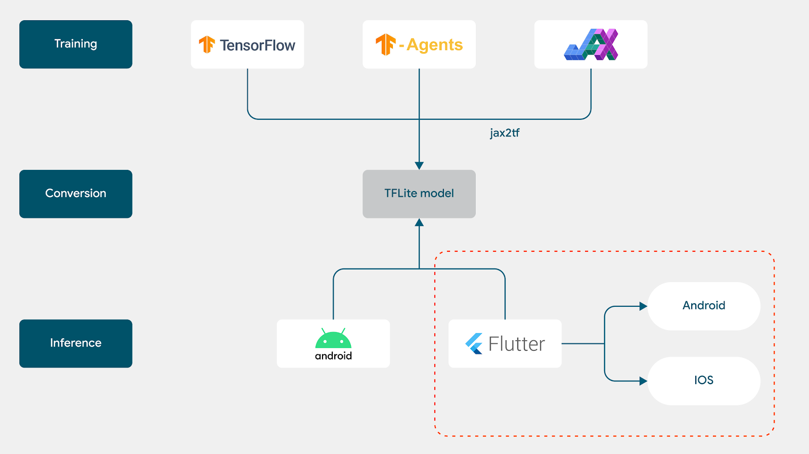
At Spotify we leverage TensorFlow and the extended TensorFlow Ecosystem (TFX, TensorFlow Serving, and so on) as part of our production Machine Learning Stack. We made the decision early on to leverage TensorFlow Agents as our RL Library of choice, knowing that integrating our experiments with our production systems would be vastly more efficient down the line.
One missing bit of technology we required was an offline Spotify environment we could use to prototype, analyze, explore, and train Agents offline prior to online testing. The flexibility of the TF-Agents library, coupled with the broader advantages of TensorFlow and its ecosystem, allowed us to cleanly design a robust and extendable offline Spotify simulator.
We based our simulator design on TF-Agents Environment primitives and using this simulator we developed, trained and evaluated sequential models for item recommendations, vanilla RL Agents (PPG, DQN) and a modified deep Q-Network, which we call the Action-Head DQN (AH-DQN), that addressed the specific challenges imposed by the large state and action space of our RL formulation.
Through live experiments we were able to show that our offline performance estimates were strongly correlated with online results. This then opened the door for large scale experimentation and application of Reinforcement Learning across Spotify, enabled by the technological foundations unlocked by TensorFlow and TF-Agents.
In this post we’ll provide more details about our RL problem and how we used TF-Agents to enable this work end to end.
The RL Loop and Simulated Users
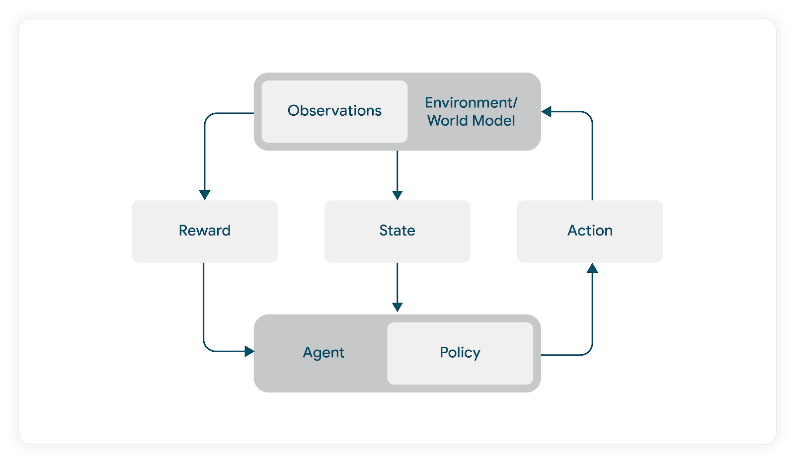
In RL, Agents interact with the environment continuously. At a given time step the Agent consumes an observation from the environment and, using this observation, produces an action given its policy at time t. The environment then processes the action and emits both a reward and the next observation (note that although typically used interchangeably, State is the complete information required to summarize the environment post action, Observation is the portion of this information actually exposed to the Agent).
In our case the reward emitted from the environment is the response of a user to music recommendations driven by the Agent’s action. In the absence of a simulator we would need to expose real users to Agents to observe rewards. We utilize a model-based RL approach to avoid letting an untrained Agent interact with real users (with the potential of hurting user satisfaction in the training process).
In this model-based RL formulation the Agent is not trained online against real users. Instead, it makes use of a user model that predicts responses to a list of tracks derived via the Agent’s action. Using this model we optimize actions in such a way as to maximize a (simulated) user satisfaction metric. During the training phase the environment makes use of this user model to return a predicted user response to the action recommended by the Agent.
We use Keras to design and train our user model. The serialized user model is then unpacked by the simulator and used to calculate rewards during Agent training and evaluation.
Simulator Design
In the abstract, what we needed to build was clear. We needed a way to simulate user listening sessions for the Agent. Given a simulated user and some content, instantiate a listening session and let the Agent drive recommendations in that session. Allow the simulated user to “react” to these recommendations and let the Agent adjust its strategy based on this result to drive some expected cumulative reward.
The TensorFlow Agents environment design guided us in developing the modular components of our system, each of which was responsible for different parts of the overall simulation.
In our codebase we define an environment abstraction that requires the following be defined for every concrete instantiation:
class AbstractEnvironment(ABC):

      _user_model: AbstractUserModel = None

      _track_sampler: AbstractTrackSampler = None

      _episode_tracker: EpisodeTracker = None

      _episode_sampler: AbstractEpisodeSampler = None
    @abstractmethod

    def reset(self) -> List[float]:

      pass
    @abstractmethod

    def step(self, action: float) -> (List[float], float, bool):

      pass
    def observation_space(self) -> Dict:

      pass
    @abstractmethod

    def action_space(self) -> Dict:

pass |
Set-Up
At the start of Agent training we need to instantiate a simulation environment that has representations of hypothetical users and the content we’re looking to recommend to them. We base these instantiations on both real and hypothetical Spotify listening experiences. The critical information that defines these instantiations is passed to the environment via _episode_sampler. As mentioned, we also need to provide the simulator with a trained user model, in this case via _user_model.
Actions and Observations
Just like any Agent environment, our simulator requires that we specify the action_spec and observation_spec. Actions in our case may be continuous or discrete depending both on our Agent selection and how we propose to translate an Agent’s action into actual recommendations. We typically recommend ordered lists of items drawn from a pool of potential items. Formulating this action space directly would lead to it being combinatorially complex. We also assume the user will interact with multiple items, and as such previous work in this area that relies on single choice assumptions doesn’t apply.
In the absence of a discrete action space consisting of item collections we need to provide the simulator with a method for turning the Agent’s action into actual recommendations. This logic is contained in the via _track_sampler. The “example play modes” proposed by the episode sampler contains information on items that can be presented to the simulated user. The track sampler consumes these and the agent’s action and returns actual item recommendations.
Termination and Reset
We also need to handle the episode termination dynamics. In our simulator, the reset rules are set by the model builder and based on empirical investigations of interaction data relevant to a specific music listening experience. As a hypothetical, we may determine that 92% of listening sessions terminate after 6 sequential track skips and we’d construct our simulation termination logic to match. It also requires that we design abstractions in our simulator that allow us to check if the episode should be terminated after each step.
When the episode is reset the simulator will sample a new hypothetical user listening session pair and begin the next episode.
Episode Steps
As with standard TF Agents Environments we need to define the step dynamics for our simulation. We have optional dynamics of the simulation that we need to make sure are enforced at each step. For example, we may desire that the same item cannot be recommended more than once. If the Agent’s action indicates a recommendation of an item that was previously recommended we need to build in the functionality to pick the next best item based on this action.
We also need to call the termination (and other supporting functions) mentioned above as needed at each step.
Episode Storage and Replay
The functionality mentioned up until this point collectively created a very complex simulation setup. While the TF Agents replay buffer provided us with the functionality required to store episodes for Agent training and evaluation, we quickly realized the need to be able to store more episode data for debugging purposes, and more detailed evaluations specific to our simulation distinct from standard Agent performance measures.
We thus allowed for the inclusion of an expanded _episode_tracker that would store additional information about the user model predictions, information noting the sampled users/content pairs, and more.
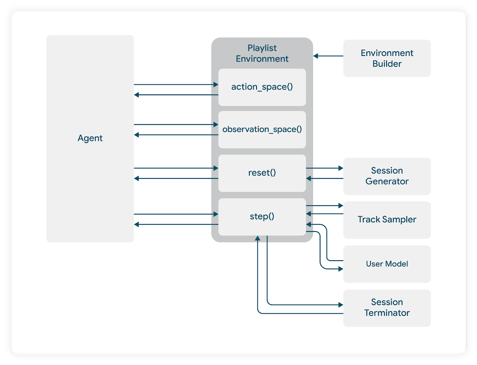
Creating TF-Agent Environments
Our environment abstraction gives us a template that matches that of a standard TF-Agents Environment class. Some inputs to our environment need to be resolved before we can actually create the concrete TF-Agents environment instance. This happens in three steps.
First we define a specific simulation environment that conforms to our abstraction. For example:
class PlaylistEnvironment(AbstractEnvironment):

    def __init__(

        self,

        user_model: AbstractUserModel,

        track_sampler: AbstractTrackSampler,

        episode_tracker: EpisodeTracker,

        episode_sampler: AbstractEpisodeSampler,

	 ....

    ):
... |
Next we use an Environment Builder Class that takes as input a user model, track sampler, etc. and an environment class like PlaylistEnvironment. The builder creates a concrete instance of this environment:
self.playlist_env: PlaylistEnvironment = environment_ctor(

            user_model=user_model,

            track_sampler=track_sampler,

            episode_tracker=episode_tracker,

            episode_sampler=self._eps_sampler,

) |
Lastly, we utilize a conversion class that constructs a TF-Agents Environment from a concrete instance of ours:
class TFAgtPyEnvironment(py_environment.PyEnvironment):

      def __init__(self, environment: AbstractEnvironment):

          super().__init__()

          self.env = environment
|
This is then executed internally to our Environment Builder:
class EnvironmentBuilder(AbstractEnvironmentBuilder):
      def __init__(self, ...):

          ...
      def get_tf_env(self):

          ...

          tf_env: TFAgtPyEnvironment = TFAgtPyEnvironment(

              self.playlist_env

              )

          return tf_env
|
The resulting TensorFlow Agents environment can then be used for Agent training.
This simulator design allows us to easily create and manage multiple environments with a variety of different configurations as needed.
We next discuss how we used our simulator to train RL Agents to generate Playlists.
A Customized Agent for Playlist Generation
As mentioned, Reinforcement Learning provides us with a method set that naturally accommodates the sequential nature of music listening; allowing us to adapt to users’ ever evolving preferences as sessions progress.
One specific problem we can attempt to use RL to solve is that of automatic music playlist generation. Given a (large) set of tracks, we want to learn how to create one optimal playlist to recommend to the user in order to maximize satisfaction metrics. Our use case is different from standard slate recommendation tasks, where usually the target is to select at most one item in the sequence. In our case, we assume we have a user-generated response for multiple items in the slate, making slate recommendation systems not directly applicable. Another complication is that the set of tracks from which recommendations are drawn is ever changing.
We designed a DQN variant capable of handling these constraints that we called an Action Head DQN (AHDQN).
The AH-DQN network takes as input the current state and an available action to produce a single Q value for the input action. This process is repeated for every possible item in the input. Finally, the item with the highest Q value is selected and added to the slate, and the process continues until the slate is full.
Experiments In Brief
We tested our approach both offline and online at scale to assess the ability of the Agent to power our real-world recommender systems. In addition to testing the Agent itself we were also keen to assess the extent to which our offline performance estimates for various policies returned by our simulator matched (or at least directionally aligned) with our online results.
We observed this directional alignment for numerous naive, heuristic, model driven, and RL policies.
Please refer to our KDD paper for more information on the specifics of our model-based RL approach and Agent design.
Federico Tomasi, Joseph Cauteruccio, Surya Kanoria, Kamil Ciosek, Matteo Rinaldi, and Zhenwen Dai
KDD 2023
Acknowledgements
We’d like to thank all our Spotify teammates past and present who contributed to this work. Particularly, we’d like to thank Mehdi Ben Ayed for his early work in helping to develop our RL codebase. We’d also like to thank the TensorFlow Agents team for their support and encouragement throughout this project (and for the library that made it possible).
Read More

 Posted by the TensorFlow team

 Posted by Sharbani Roy – Senior Director, Product Management, Google


 Posted by Google: Mathieu Guillame-Bert, Richard Stotz, Robert Crowe, Luiz GUStavo Martins (Gus), Ashley Oldacre, Kris Tonthat, Glenn Cameron, and Tryolabs: Ian Spektor, Braulio Rios, Guillermo Etchebarne, Diego Marvid, Lucas Micol, Gonzalo Marín, Alan Descoins, Agustina Pizarro, Lucía Aguilar, Martin Alcala Rubi


 Posted by

 Posted by


 Posted by