In 2021, we launched AWS Support Proactive Services as part of the AWS Enterprise Support plan. Since its introduction, we have helped hundreds of customers optimize their workloads, set guardrails, and improve visibility of their machine learning (ML) workloads’ cost and usage.
In this series of posts, we share lessons learned about optimizing costs in Amazon SageMaker. In Part 1, we showed how to get started using AWS Cost Explorer to identify cost optimization opportunities in SageMaker. In this post, we focus on SageMaker inference environments: real-time inference, batch transform, asynchronous inference, and serverless inference.
| Analyze Amazon SageMaker spend and determine cost optimization opportunities based on usage:
|
SageMaker offers multiple inference options for you to pick from based on your workload requirements:
- Real-time inference for online, low latency, or high throughput requirements
- Batch transform for offline, scheduled processing and when you don’t need a persistent endpoint
- Asynchronous inference for when you have large payloads with long processing times and want to queue requests
- Serverless inference for when you have intermittent or unpredictable traffic patterns and can tolerate cold starts
In the following sections, we discuss each inference option in more detail.
SageMaker real-time inference
When you create an endpoint, SageMaker attaches an Amazon Elastic Block Store (Amazon EBS) storage volume to the Amazon Elastic Compute Cloud (Amazon EC2) instance that hosts the endpoint. This is true for all instance types that don’t come with a SSD storage. Because the d* instance types come with an NVMe SSD storage, SageMaker doesn’t attach an EBS storage volume to these ML compute instances. Refer to Host instance storage volumes for the size of the storage volumes that SageMaker attaches for each instance type for a single endpoint and for a multi-model endpoint.
The cost of SageMaker real-time endpoints is based on the per instance-hour consumed for each instance while the endpoint is running, the cost of GB-month of provisioned storage (EBS volume), as well as the GB data processed in and out of the endpoint instance, as outlined in Amazon SageMaker Pricing. In Cost Explorer, you can view real-time endpoint costs by applying a filter on the usage type. The names of these usage types are structured as follows:
REGION-Host:instanceType (for example, USE1-Host:ml.c5.9xlarge)REGION-Host:VolumeUsage.gp2 (for example, USE1-Host:VolumeUsage.gp2)REGION-Hst:Data-Bytes-Out (for example, USE2-Hst:Data-Bytes-In)REGION-Hst:Data-Bytes-Out (for example, USW2-Hst:Data-Bytes-Out)
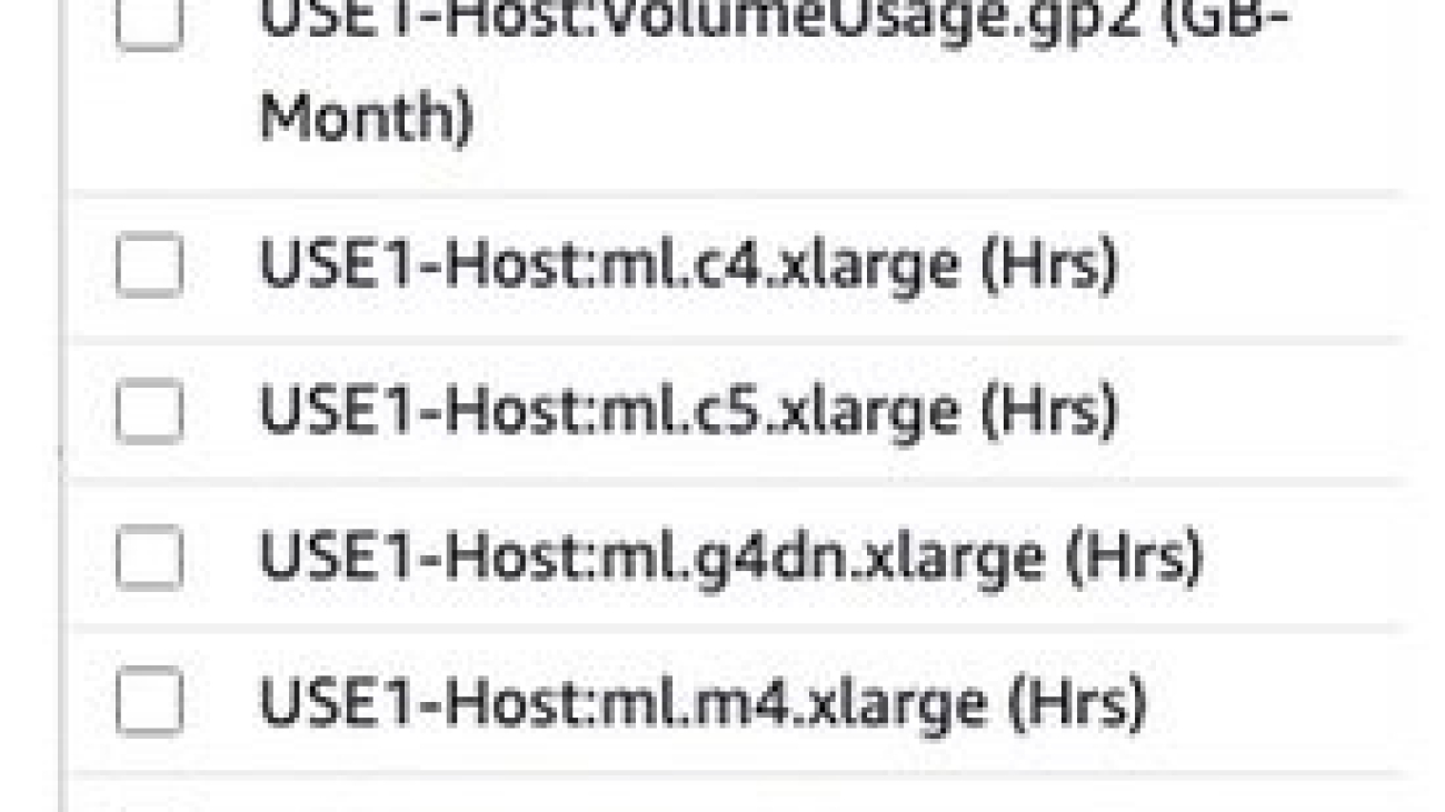
As shown in the following screenshot, filtering by the usage type Host: will show a list of real-time hosting usage types in an account.
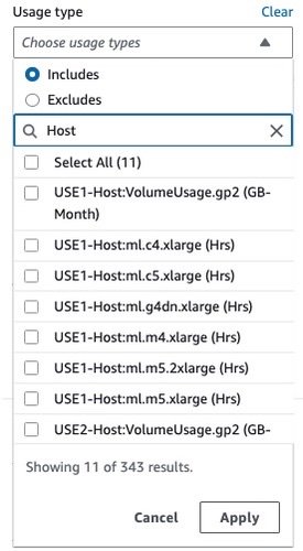
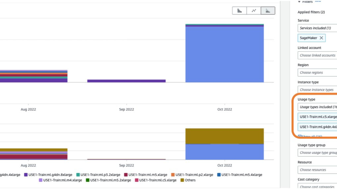
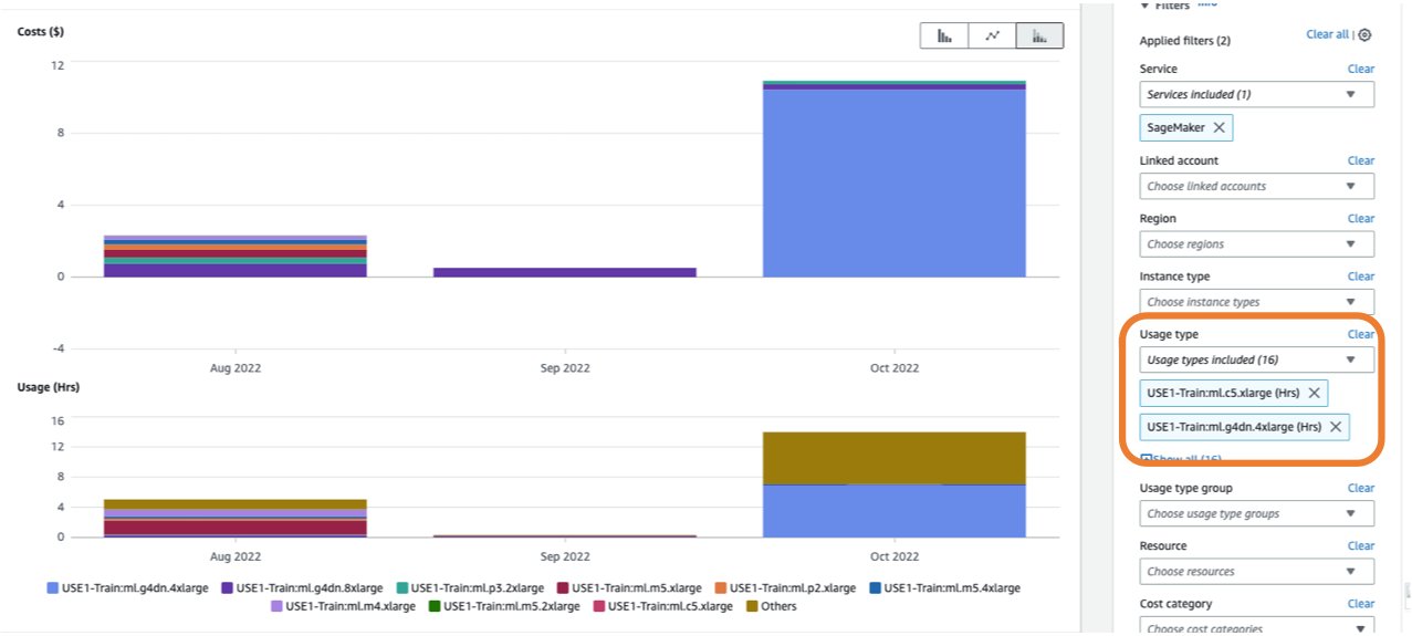
You can either select specific usage types or select Select All and choose Apply to display the cost breakdown of SageMaker real-time hosting usage. To see the cost and usage breakdown by instance hours, you need to de-select all the REGION-Host:VolumeUsage.gp2 usage types before applying the usage type filter. You can also apply additional filters such as account number, EC2 instance type, cost allocation tag, Region, and more. The following screenshot shows cost and usage graphs for the selected hosting usage types.
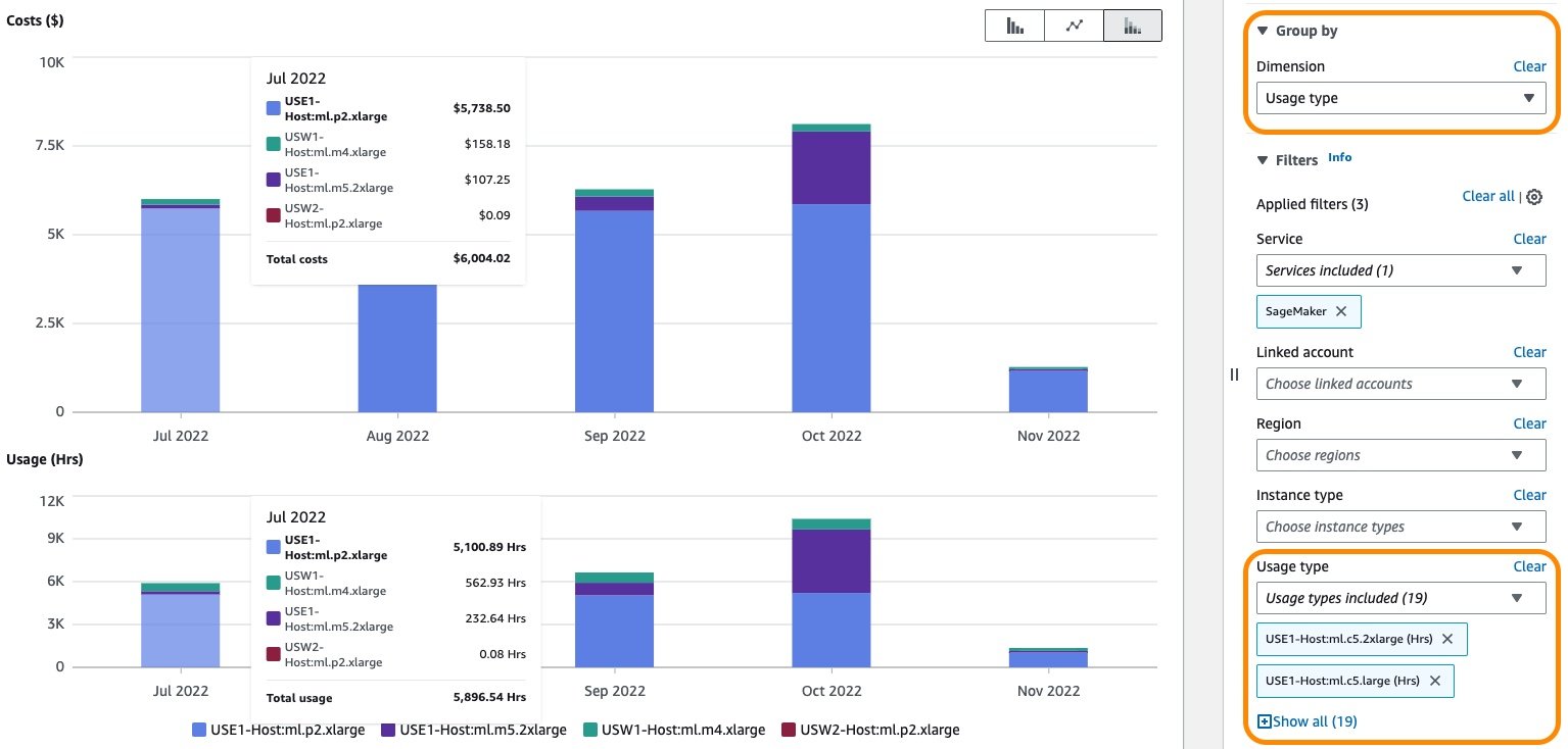
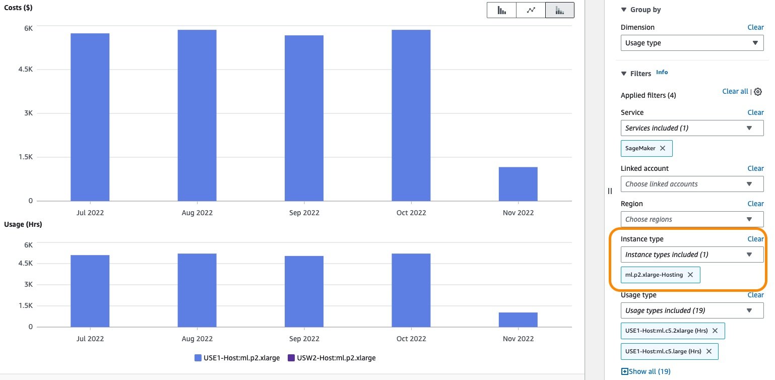
Additionally, you can explore the cost associated with one or more hosting instances by using the Instance type filter. The following screenshot shows cost and usage breakdown for hosting instance ml.p2.xlarge.
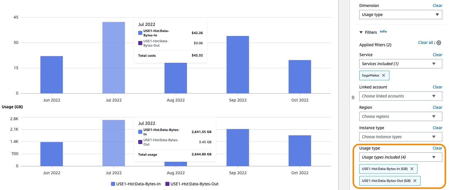
Similarly, the cost for GB data processed in and processed out can be displayed by selecting the associated usage types as an applied filter, as shown in the following screenshot.
After you have achieved your desired results with filters and groupings, you can either download your results by choosing Download as CSV or save the report by choosing Save to report library. For general guidance on using Cost Explorer, refer to AWS Cost Explorer’s New Look and Common Use Cases.
Optionally, you can enable AWS Cost and Usage Reports (AWS CUR) to gain insights into the cost and usage data for your accounts. AWS CUR contains hourly AWS consumption details. It’s stored in Amazon Simple Storage Service (Amazon S3) in the payer account, which consolidates data for all the linked accounts. You can run queries to analyze trends in your usage and take appropriate action to optimize cost. Amazon Athena is a serverless query service that you can use to analyze the data from AWS CUR in Amazon S3 using standard SQL. More information and example queries can be found in the AWS CUR Query Library.
You can also feed AWS CUR data into Amazon QuickSight, where you can slice and dice it any way you’d like for reporting or visualization purposes. For instructions, see How do I ingest and visualize the AWS Cost and Usage Report (CUR) into Amazon QuickSight.
You can obtain resource-level information such as endpoint ARN, endpoint instance types, hourly instance rate, daily usage hours, and more from AWS CUR. You can also include cost-allocation tags in your query for an additional level of granularity. The following example query returns real-time hosting resource usage for the last 3 months for the given payer account:
SELECT
      bill_payer_account_id,
      line_item_usage_account_id,
      line_item_resource_id AS endpoint_arn,
      line_item_usage_type,
      DATE_FORMAT((line_item_usage_start_date),'%Y-%m-%d') AS day_line_item_usage_start_date,
      SUM(CAST(line_item_usage_amount AS DOUBLE)) AS sum_line_item_usage_amount,
      line_item_unblended_rate,
      SUM(CAST(line_item_unblended_cost AS DECIMAL(16,8))) AS sum_line_item_unblended_cost,
      line_item_blended_rate,
      SUM(CAST(line_item_blended_cost AS DECIMAL(16,8))) AS sum_line_item_blended_cost,
      line_item_line_item_description,
      line_item_line_item_type
    FROM
      customer_all
    WHERE
      line_item_usage_start_date >= date_trunc('month',current_date - interval '3' month)
      AND line_item_product_code = 'AmazonSageMaker'
      AND line_item_line_item_type  IN ('DiscountedUsage', 'Usage', 'SavingsPlanCoveredUsage')
      AND line_item_usage_type like '%Host%'
        AND line_item_operation = 'RunInstance'
        AND bill_payer_account_id = 'xxxxxxxxxxxx'
    GROUP BY
      bill_payer_account_id,
      line_item_usage_account_id,
      line_item_resource_id,
      line_item_usage_type,
      line_item_unblended_rate,
      line_item_blended_rate,
      line_item_line_item_type,
      DATE_FORMAT((line_item_usage_start_date),'%Y-%m-%d'),
      line_item_line_item_description
      ORDER BY
      line_item_resource_id, day_line_item_usage_start_date
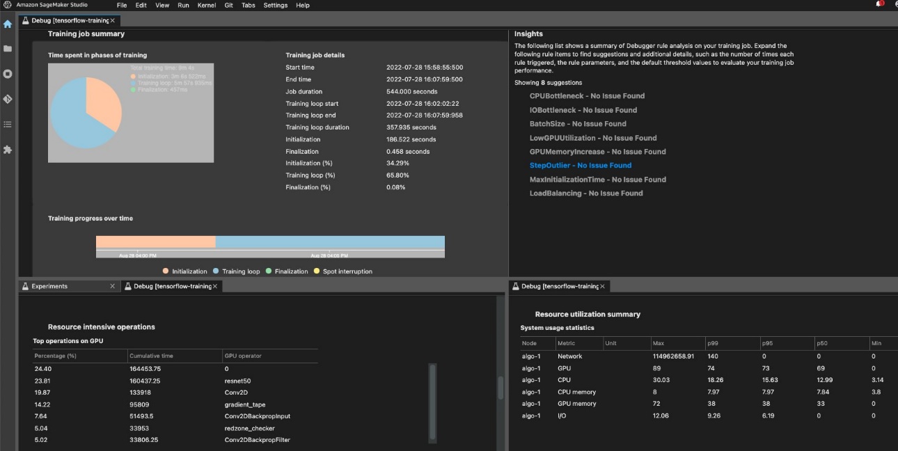
The following screenshot shows the results obtained from running the query using Athena. For more information, refer to Querying Cost and Usage Reports using Amazon Athena.

The result of the query shows that endpoint mme-xgboost-housing with ml.x4.xlarge instance is reporting 24 hours of runtime for multiple consecutive days. The instance rate is $0.24/hour and the daily cost for running for 24 hours is $5.76.
AWS CUR results can help you identify patterns of endpoints running for consecutive days in each of the linked accounts, as well as endpoints with the highest monthly cost. This can also help you decide whether the endpoints in non-production accounts can be deleted to save cost.
Optimize costs for real-time endpoints
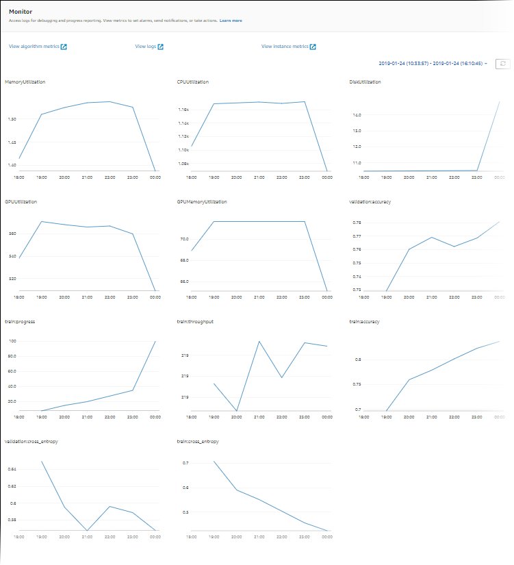
From a cost management perspective, it’s important to identify under-utilized (or over-sized) instances and bring the instance size and counts, if required, in line with workload requirements. Common system metrics like CPU/GPU utilization and memory utilization are written to Amazon CloudWatch for all hosting instances. For real-time endpoints, SageMaker makes several additional metrics available in CloudWatch. Some of the commonly monitored metrics include invocation counts and invocation 4xx/5xx errors. For a full list of metrics, refer to Monitor Amazon SageMaker with Amazon CloudWatch.
The metric CPUUtilization provides the sum of each individual CPU core’s utilization. The CPU utilization of each core range is 0–100. For example, if there are four CPUs, the CPUUtilization range is 0–400%. The metric MemoryUtilization is the percentage of memory that is used by the containers on an instance. This value range is 0–100%. The following screenshot shows an example of CloudWatch metrics CPUUtilization and MemoryUtilization for an endpoint instance ml.m4.10xlarge that comes with 40 vCPUs and 160 GiB memory.
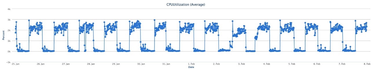
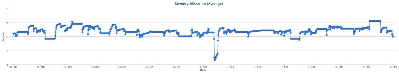
These metrics graphs show maximum CPU utilization of approximately 3,000%, which is the equivalent of 30 vCPUs. This means that this endpoint isn’t utilizing more than 30 vCPUs out of the total capacity of 40 vCPUs. Similarly, the memory utilization is below 6%. Using this information, you can possibly experiment with a smaller instance that can match this resource need. Furthermore, the CPUUtilization metric shows a classic pattern of periodic high and low CPU demand, which makes this endpoint a good candidate for auto scaling. You can start with a smaller instance and scale out first as your compute demand changes. For information, see Automatically Scale Amazon SageMaker Models.
SageMaker is great for testing new models because you can easily deploy them into an A/B testing environment using production variants, and you only pay for what you use. Each production variant runs on its own compute instance and you’re charged per instance-hour consumed for each instance while the variant is running.
SageMaker also supports shadow variants, which have the same components as a production variant and run on their own compute instance. With shadow variants, SageMaker automatically deploys the model in a test environment, routes a copy of the inference requests received by the production model to the test model in real time, and collects performance metrics such as latency and throughput. This enables you to validate any new candidate component of your model serving stack before promoting it to production.
When you’re done with your tests and aren’t using the endpoint or the variants extensively anymore, you should delete it to save cost. Because the model is stored in Amazon S3, you can recreate it as needed. You can automatically detect these endpoints and take corrective actions (such as deleting them) by using Amazon CloudWatch Events and AWS Lambda functions. For example, you can use the Invocations metric to get the total number of requests sent to a model endpoint and then detect if the endpoints have been idle for the past number of hours (with no invocations over a certain period, such as 24 hours).
If you have several under-utilized endpoint instances, consider hosting options such as multi-model endpoints (MMEs), multi-container endpoints (MCEs), and serial inference pipelines to consolidate usage to fewer endpoint instances.
For real-time and asynchronous inference model deployment, you can optimize cost and performance by deploying models on SageMaker using AWS Graviton. AWS Graviton is a family of processors designed by AWS that provide the best price performance and are more energy efficient than their x86 counterparts. For guidance on deploying an ML model to AWS Graviton-based instances and details on the price performance benefit, refer to Run machine learning inference workloads on AWS Graviton-based instances with Amazon SageMaker. SageMaker also supports AWS Inferentia accelerators through the ml.inf2 family of instances for deploying ML models for real-time and asynchronous inference. You can use these instances on SageMaker to achieve high performance at a low cost for generative artificial intelligence (AI) models, including large language models (LLMs) and vision transformers.
In addition, you can use Amazon SageMaker Inference Recommender to run load tests and evaluate the price performance benefits of deploying your model on these instances. For additional guidance on automatically detecting idle SageMaker endpoints, as well as instance right-sizing and auto scaling for SageMaker endpoints, refer to Ensure efficient compute resources on Amazon SageMaker.
SageMaker batch transform
Batch inference, or offline inference, is the process of generating predictions on a batch of observations. Offline predictions are suitable for larger datasets and in cases where you can afford to wait several minutes or hours for a response.
The cost for SageMaker batch transform is based on the per instance-hour consumed for each instance while the batch transform job is running, as outlined in Amazon SageMaker Pricing. In Cost Explorer, you can explore batch transform costs by applying a filter on the usage type. The name of this usage type is structured as REGION-Tsform:instanceType (for example, USE1-Tsform:ml.c5.9xlarge).
As shown in the following screenshot, filtering by usage type Tsform: will show a list of SageMaker batch transform usage types in an account.
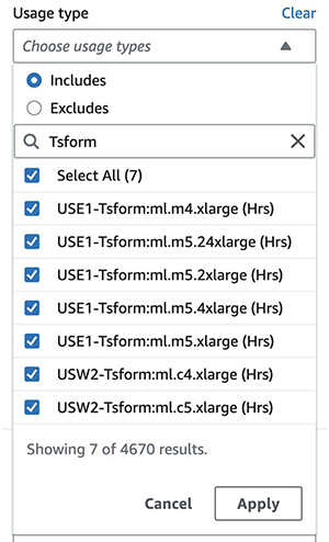
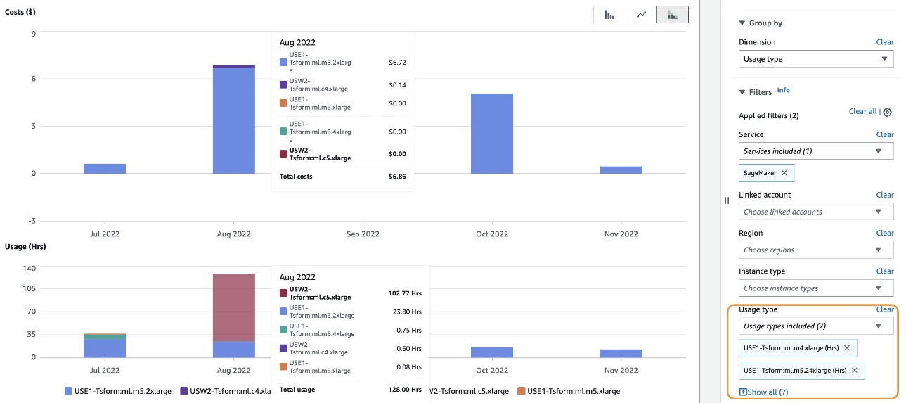
You can either select specific usage types or select Select All and choose Apply to display the cost breakdown of batch transform instance usage for the selected types. As mentioned earlier, you can also apply additional filters. The following screenshot shows cost and usage graphs for the selected batch transform usage types.
Optimize costs for batch transform
SageMaker batch transform only charges you for the instances used while your jobs are running. If your data is already in Amazon S3, then there is no cost for reading input data from Amazon S3 and writing output data to Amazon S3. All output objects are attempted to be uploaded to Amazon S3. If all are successful, then the batch transform job is marked as complete. If one or more objects fail, the batch transform job is marked as failed.
Charges for batch transform jobs apply in the following scenarios:
- The job is successful
- Failure due to
ClientError and the model container is SageMaker or a SageMaker managed framework
- Failure due to
AlgorithmError or ClientError and the model container is your own custom container (BYOC)
The following are some of the best practices for optimizing a SageMaker batch transform job. These recommendations can reduce the total runtime of your batch transform job, thereby lowering costs:
- Set BatchStrategy to
MultiRecord and SplitType to Line if you need the batch transform job to make mini batches from the input file. If it can’t automatically split the dataset into mini batches, you can divide it into mini batches by putting each batch in a separate input file, placed in the data source S3 bucket.
- Make sure that the batch size fits into the memory. SageMaker usually handles this automatically; however, when dividing batches manually, this needs to be tuned based on the memory.
- Batch transform partitions the S3 objects in the input by key and maps those objects to instances. When you have multiples files, one instance might process
input1.csv, and another instance might process input2.csv. If you have one input file but initialize multiple compute instances, only one instance processes the input file and the rest of the instances are idle. Make sure the number of files is equal to or greater than the number of instances.
- If you have a large number of small files, it may be beneficial to combine multiple files into a small number of bigger files to reduce Amazon S3 interaction time.
- If you’re using the CreateTransformJob API, you can reduce the time it takes to complete batch transform jobs by using optimal values for parameters such as MaxPayloadInMB, MaxConcurrentTransforms, or BatchStrategy:
MaxConcurrentTransforms indicates the maximum number of parallel requests that can be sent to each instance in a transform job. The ideal value for MaxConcurrentTransforms is equal to the number of vCPU cores in an instance.MaxPayloadInMB is the maximum allowed size of the payload, in MB. The value in MaxPayloadInMB must be greater than or equal to the size of a single record. To estimate the size of a record in MB, divide the size of your dataset by the number of records. To ensure that the records fit within the maximum payload size, we recommend using a slightly larger value. The default value is 6 MB.MaxPayloadInMB must not be greater than 100 MB. If you specify the optional MaxConcurrentTransforms parameter, then the value of (MaxConcurrentTransforms * MaxPayloadInMB) must also not exceed 100 MB.- For cases where the payload might be arbitrarily large and is transmitted using HTTP chunked encoding, set the MaxPayloadInMB value to 0. This feature works only in supported algorithms. Currently, SageMaker built-in algorithms do not support HTTP chunked encoding.
- Batch inference tasks are usually good candidates for horizontal scaling. Each worker within a cluster can operate on a different subset of data without the need to exchange information with other workers. AWS offers multiple storage and compute options that enable horizontal scaling. If a single instance is not sufficient to meet your performance requirements, consider using multiple instances in parallel to distribute the workload. For key considerations when architecting batch transform jobs, refer to Batch Inference at Scale with Amazon SageMaker.
- Continuously monitor the performance metrics of your SageMaker batch transform jobs using CloudWatch. Look for bottlenecks, such as high CPU or GPU utilization, memory usage, or network throughput, to determine if you need to adjust instance sizes or configurations.
- SageMaker uses the Amazon S3 multipart upload API to upload results from a batch transform job to Amazon S3. If an error occurs, the uploaded results are removed from Amazon S3. In some cases, such as when a network outage occurs, an incomplete multipart upload might remain in Amazon S3. To avoid incurring storage charges, we recommend that you add the S3 bucket policy to the S3 bucket lifecycle rules. This policy deletes incomplete multipart uploads that might be stored in the S3 bucket. For more information, see Managing your storage lifecycle.
SageMaker asynchronous inference
Asynchronous inference is a great choice for cost-sensitive workloads with large payloads and burst traffic. Requests can take up to 1 hour to process and have payload sizes of up to 1 GB, so it’s more suitable for workloads that have relaxed latency requirements.
Invocation of asynchronous endpoints differs from real-time endpoints. Rather than passing a request payload synchronously with the request, you upload the payload to Amazon S3 and pass an S3 URI as a part of the request. Internally, SageMaker maintains a queue with these requests and processes them. During endpoint creation, you can optionally specify an Amazon Simple Notification Service (Amazon SNS) topic to receive success or error notifications. When you receive the notification that your inference request has been successfully processed, you can access the result in the output Amazon S3 location.
The cost for asynchronous inference is based on the per instance-hour consumed for each instance while the endpoint is running, cost of GB-month of provisioned storage, as well as GB data processed in and out of the endpoint instance, as outlined in Amazon SageMaker Pricing. In Cost Explorer, you can filter asynchronous inference costs by applying a filter on the usage type. The name of this usage type is structured as REGION-AsyncInf:instanceType (for example, USE1-AsyncInf:ml.c5.9xlarge). Note that GB volume and GB data processed usage types are the same as real-time endpoints, as mentioned earlier in this post.
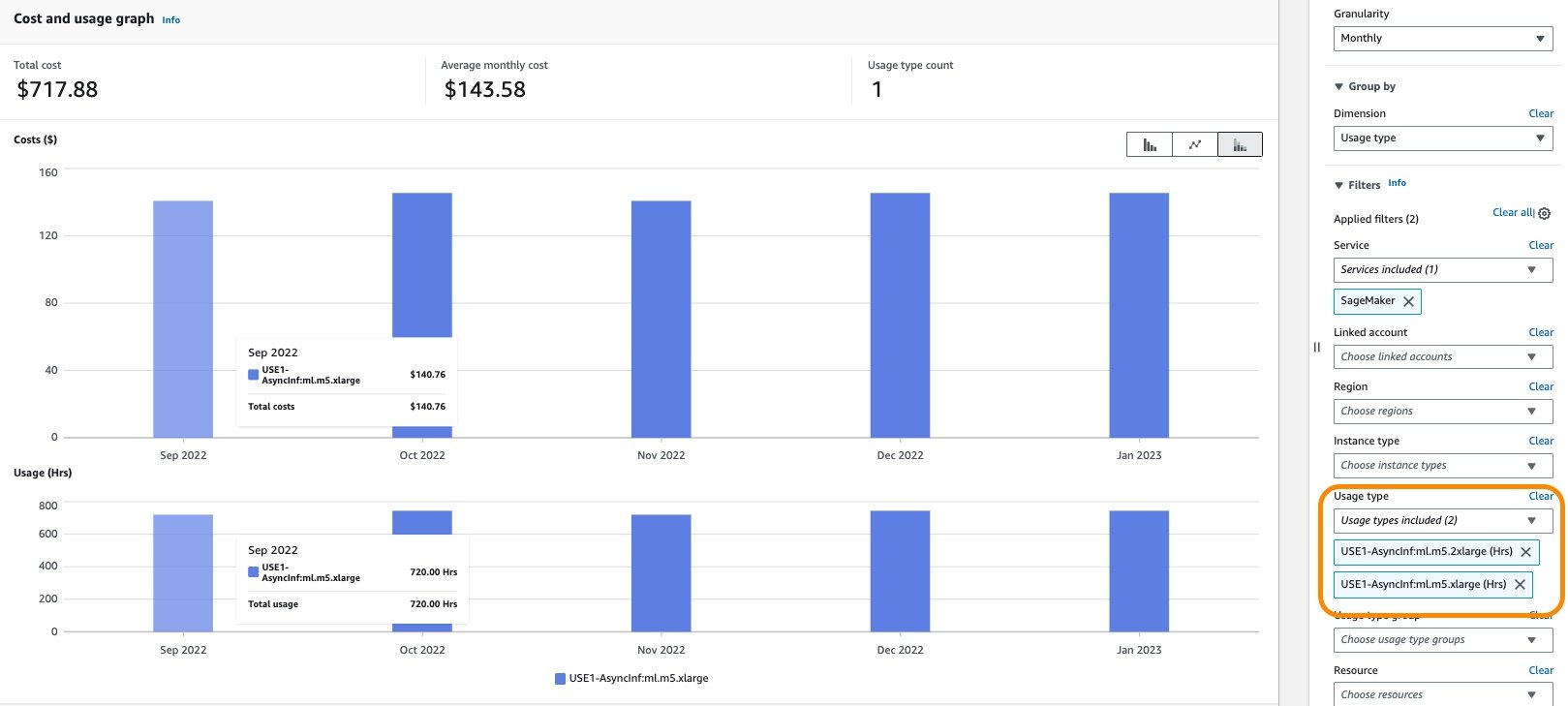
As shown in the following screenshot, filtering by the usage type AsyncInf: in Cost Explorer displays a cost breakdown by asynchronous endpoint usage types.
To see the cost and usage breakdown by instance hours, you need to de-select all the REGION-Host:VolumeUsage.gp2 usage types before applying the usage type filter. You can also apply additional filters. Resource-level information such as endpoint ARN, endpoint instance types, hourly instance rate, and daily usage hours can be obtained from AWS CUR. The following is an example of an AWS CUR query to obtain asynchronous hosting resource usage for the last 3 months:
SELECT
      bill_payer_account_id,
      line_item_usage_account_id,
      line_item_resource_id AS endpoint_arn,
      line_item_usage_type,
      DATE_FORMAT((line_item_usage_start_date),'%Y-%m-%d') AS day_line_item_usage_start_date,
      SUM(CAST(line_item_usage_amount AS DOUBLE)) AS sum_line_item_usage_amount,
      line_item_unblended_rate,
      SUM(CAST(line_item_unblended_cost AS DECIMAL(16,8))) AS sum_line_item_unblended_cost,
      line_item_blended_rate,
      SUM(CAST(line_item_blended_cost AS DECIMAL(16,8))) AS sum_line_item_blended_cost,
      line_item_line_item_description,
      line_item_line_item_type
    FROM
      customer_all
    WHERE
      line_item_usage_start_date >= date_trunc('month',current_date - interval '3' month)
      AND line_item_product_code = 'AmazonSageMaker'
      AND line_item_line_item_type  IN ('DiscountedUsage', 'Usage', 'SavingsPlanCoveredUsage')
      AND line_item_usage_type like '%AsyncInf%'
      AND line_item_operation = 'RunInstance'
    GROUP BY
      bill_payer_account_id,
      line_item_usage_account_id,
      line_item_resource_id,
      line_item_usage_type,
      line_item_unblended_rate,
      line_item_blended_rate,
      line_item_line_item_type,
      DATE_FORMAT((line_item_usage_start_date),'%Y-%m-%d'),
      line_item_line_item_description
      ORDER BY
      line_item_resource_id, day_line_item_usage_start_date
The following screenshot shows the results obtained from running the AWS CUR query using Athena.
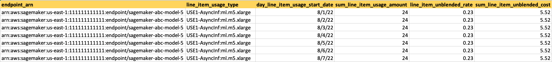
The result of the query shows that endpoint sagemaker-abc-model-5 with ml.m5.xlarge instance is reporting 24 hours of runtime for multiple consecutive days. The instance rate is $0.23/hour and the daily cost for running for 24 hours is $5.52.
As mentioned earlier, AWS CUR results can help you identify patterns of endpoints running for consecutive days, as well as endpoints with the highest monthly cost. This can also help you decide whether the endpoints in non-production accounts can be deleted to save cost.
Optimize costs for asynchronous inference
Just like the real-time endpoints, the cost for asynchronous endpoints is based on the instance type usage. Therefore, it’s important to identify under-utilized instances and resize them based on the workload requirements. In order to monitor asynchronous endpoints, SageMaker makes several metrics such as ApproximateBacklogSize, HasBacklogWithoutCapacity, and more available in CloudWatch. These metrics can show requests in the queue for an instance and can be used for auto scaling an endpoint. SageMaker asynchronous inference also includes host-level metrics. For information on host-level metrics, see SageMaker Jobs and Endpoint Metrics. These metrics can show resource utilization that can help you right-size the instance.
SageMaker supports auto scaling for asynchronous endpoints. Unlike real-time hosted endpoints, asynchronous inference endpoints support scaling down instances to zero by setting the minimum capacity to zero. For asynchronous endpoints, SageMaker strongly recommends that you create a policy configuration for target-tracking scaling for a deployed model (variant). You need to define the scaling policy that scaled on the ApproximateBacklogPerInstance custom metric and set the MinCapacity value to zero.
Asynchronous inference enables you to save on costs by auto scaling the instance count to zero when there are no requests to process, so you only pay when your endpoint is processing requests. Requests that are received when there are zero instances are queued for processing after the endpoint scales up. Therefore, for use cases that can tolerate a cold start penalty of a few minutes, you can optionally scale down the endpoint instance count to zero when there are no outstanding requests and scale back up as new requests arrive. Cold start time depends on the time required to launch a new endpoint from scratch. Also, if the model itself is big, then the time can be longer. If your job is expected to take longer than the 1-hour processing time, you may want to consider SageMaker batch transform.
Additionally, you may also consider your request’s queued time combined with the processing time to choose the instance type. For example, if your use case can tolerate hours of wait time, you can choose a smaller instance to save cost.
For additional guidance on instance right-sizing and auto scaling for SageMaker endpoints, refer to Ensure efficient compute resources on Amazon SageMaker.
Serverless inference
Serverless inference allows you to deploy ML models for inference without having to configure or manage the underlying infrastructure. Based on the volume of inference requests your model receives, SageMaker serverless inference automatically provisions, scales, and turns off compute capacity. As a result, you pay for only the compute time to run your inference code and the amount of data processed, not for idle time. For serverless endpoints, instance provisioning is not necessary. You need to provide the memory size and maximum concurrency. Because serverless endpoints provision compute resources on demand, your endpoint may experience a few extra seconds of latency (cold start) for the first invocation after an idle period. You pay for the compute capacity used to process inference requests, billed by the millisecond, GB-month of provisioned storage, and the amount of data processed. The compute charge depends on the memory configuration you choose.
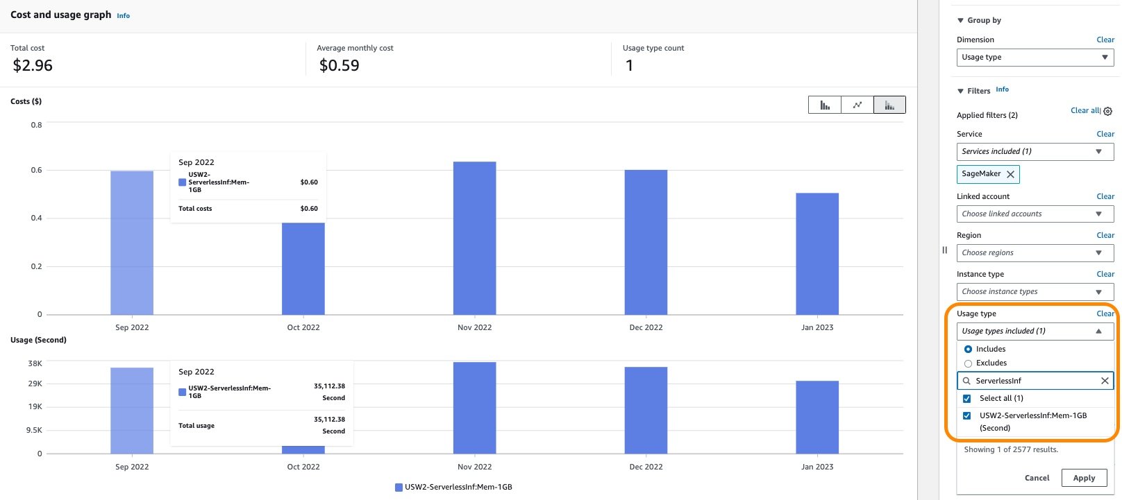
In Cost Explorer, you can filter serverless endpoints costs by applying a filter on the usage type. The name of this usage type is structured as REGION-ServerlessInf:Mem-MemorySize (for example, USE2-ServerlessInf:Mem-4GB). Note that GB volume and GB data processed usage types are the same as real-time endpoints.
You can see the cost breakdown by applying additional filters such as account number, instance type, Region, and more. The following screenshot shows the cost breakdown by applying filters for the serverless inference usage type.
Optimize cost for serverless inference
When configuring your serverless endpoint, you can specify the memory size and maximum number of concurrent invocations. SageMaker serverless inference auto-assigns compute resources proportional to the memory you select. If you choose a larger memory size, your container has access to more vCPUs. With serverless inference, you only pay for the compute capacity used to process inference requests, billed by the millisecond, and the amount of data processed. The compute charge depends on the memory configuration you choose. The memory sizes you can choose are 1024 MB, 2048 MB, 3072 MB, 4096 MB, 5120 MB, and 6144 MB. The pricing increases with the memory size increments, as explained in Amazon SageMaker Pricing, so it’s important to select the correct memory size. As a general rule, the memory size should be at least as large as your model size. However, it’s a good practice to refer to memory utilization when deciding the endpoint memory size, in addition to the model size itself.
General best practices for optimizing SageMaker inference costs
Optimizing hosting costs isn’t a one-time event. It’s a continuous process of monitoring deployed infrastructure, usage patterns, and performance, and also keeping a keen eye on new innovative solutions that AWS releases that could impact cost. Consider the following best practices:
- Choose an appropriate instance type – SageMaker supports multiple instance types, each with varying combinations of CPU, GPU, memory, and storage capacities. Based on your model’s resource requirements, choose an instance type that provides the necessary resources without over-provisioning. For information about available SageMaker instance types, their specifications, and guidance on selecting the right instance, refer to Ensure efficient compute resources on Amazon SageMaker.
- Test using local mode – In order to detect failures and debug faster, it’s recommended to test the code and container (in case of BYOC) in local mode before running the inference workload on the remote SageMaker instance. Local mode is a great way to test your scripts before running them in a SageMaker managed hosting environment.
- Optimize models to be more performant – Unoptimized models can lead to longer runtimes and use more resources. You can choose to use more or bigger instances to improve performance; however, this leads to higher costs. By optimizing your models to be more performant, you may be able to lower costs by using fewer or smaller instances while keeping the same or better performance characteristics. You can use Amazon SageMaker Neo with SageMaker inference to automatically optimize models. For more details and samples, see Optimize model performance using Neo.
- Use tags and cost management tools – To maintain visibility into your inference workloads, it’s recommended to use tags as well as AWS cost management tools such as AWS Budgets, the AWS Billing console, and the forecasting feature of Cost Explorer. You can also explore SageMaker Savings Plans as a flexible pricing model. For more information about these options, refer to Part 1 of this series.
Conclusion
In this post, we provided guidance on cost analysis and best practices when using SageMaker inference options. As machine learning establishes itself as a powerful tool across industries, training and running ML models needs to remain cost-effective. SageMaker offers a wide and deep feature set for facilitating each step in the ML pipeline and provides cost optimization opportunities without impacting performance or agility. Reach out to your AWS team for cost guidance on your SageMaker workloads.
| Refer to the following posts in this series for more information about optimizing cost for SageMaker:
|
About the Authors
 Deepali Rajale is a Senior AI/ML Specialist at AWS. She works with enterprise customers providing technical guidance with best practices for deploying and maintaining AI/ML solutions in the AWS ecosystem. She has worked with a wide range of organizations on various deep learning use cases involving NLP and computer vision. She is passionate about empowering organizations to leverage generative AI to enhance their use experience. In her spare time, she enjoys movies, music, and literature.
 Uri Rosenberg is the AI & ML Specialist Technical Manager for Europe, Middle East, and Africa. Based out of Israel, Uri works to empower enterprise customers on all things ML to design, build, and operate at scale. In his spare time, he enjoys cycling, hiking, and rock and roll climbing.
Read More


 Sathya Balakrishnan is a Senior Consultant in the Professional Services team at AWS, specializing in data and ML solutions. He works with US federal financial clients. He is passionate about building pragmatic solutions to solve customers’ business problems. In his spare time, he enjoys watching movies and hiking with his family.
 RG Thiyagarajan is a Senior Consultant in Professional Services at AWS, specializing in application migration, security, and resiliency with US federal financial clients.
 Sid Padgaonkar is the Senior Product Manager for Amazon Translate, AWS’s natural language processing service. On weekends, you will find him playing squash and exploring the food scene in the Pacific Northwest.
 Guilherme Ricci is a Senior Startup Solutions Architect on Amazon Web Services, helping startups modernize and optimize the costs of their applications. With over 10 years of experience with companies in the financial sector, he is currently working with a team of AI/ML specialists.
 Evandro Franco is an AI/ML Specialist Solutions Architect working on Amazon Web Services. He helps AWS customers overcome business challenges related to AI/ML on top of AWS. He has more than 15 years working with technology, from software development, infrastructure, serverless, to machine learning.
 Matthew McClean leads the Annapurna ML Solution Architecture team that helps customers adopt AWS Trainium and AWS Inferentia products. He is passionate about generative AI and has been helping customers adopt AWS technologies for the last 10 years.


 Neelam Koshiya is an Enterprise Solutions Architect at AWS. With a background in software engineering, she organically moved into an architecture role. Her current focus is helping enterprise customers with their cloud adoption journey for strategic business outcomes with the area of depth being AI/ML. She is passionate about innovation and inclusion. In her spare time, she enjoys reading and being outdoors.
 João Moura is an AI/ML Specialist Solutions Architect at AWS, based in Spain. He helps customers with deep learning model training and inference optimization, and more broadly building large-scale ML platforms on AWS. He is also an active proponent of ML-specialized hardware and low-code ML solutions.


 Giuseppe Angelo Porcelli is a Principal Machine Learning Specialist Solutions Architect for Amazon Web Services. With several years software engineering an ML background, he works with customers of any size to deeply understand their business and technical needs and design AI and Machine Learning solutions that make the best use of the AWS Cloud and the Amazon Machine Learning stack. He has worked on projects in different domains, including MLOps, Computer Vision, NLP, and involving a broad set of AWS services. In his free time, Giuseppe enjoys playing football.
 Bruno Pistone is an AI/ML Specialist Solutions Architect for AWS based in Milan. He works with customers of any size on helping them to deeply understand their technical needs and design AI and Machine Learning solutions that make the best use of the AWS Cloud and the Amazon Machine Learning stack. His field of expertise are Machine Learning end to end, Machine Learning Industrialization and MLOps. He enjoys spending time with his friends and exploring new places, as well as travelling to new destinations.
 Durga Sury is an ML Solutions Architect on the Amazon SageMaker Service SA team. She is passionate about making machine learning accessible to everyone. In her 4 years at AWS, she has helped set up AI/ML platforms for enterprise customers. When she isn’t working, she loves motorcycle rides, mystery novels, and long walks with her 5-year-old husky.


 Eitan Sela is a Machine Learning Specialist Solutions Architect with Amazon Web Services. He works with AWS customers to provide guidance and technical assistance, helping them build and operate machine learning solutions on AWS. In his spare time, Eitan enjoys jogging and reading the latest machine learning articles.

 Dhiraj Thakur is a Solutions Architect with Amazon Web Services. He works with AWS customers and partners to provide guidance on enterprise cloud adoption, migration, and strategy. He is passionate about technology and enjoys building and experimenting in the analytics and AI/ML space.
 Dewan Choudhury is a Software Development Engineer with Amazon Web Services. He works on Amazon SageMaker’s algorithms and JumpStart offerings. Apart from building AI/ML infrastructures, he is also passionate about building scalable distributed systems.
 Dr. Xin Huang is an Applied Scientist for Amazon SageMaker JumpStart and Amazon SageMaker built-in algorithms. He focuses on developing scalable machine learning algorithms. His research interests are in the area of natural language processing, explainable deep learning on tabular data, and robust analysis of non-parametric space-time clustering. He has published many papers in ACL, ICDM, KDD conferences, and Royal Statistical Society: Series A journal.
 Tony Cruz