Monthly Archives: May 2023

Text-to-image generation is a task in which a machine learning (ML) model generates an image from a textual description. The goal is to generate an image that closely matches the description, capturing the details and nuances of the text. This task is challenging because it requires the model to understand the semantics and syntax of the text and to generate photorealistic images. There are many practical applications of text-to-image generation in AI photography, concept art, building architecture, fashion, video games, graphic design, and much more.

Stable Diffusion is a text-to-image model that empowers you to create high-quality images within seconds. When real-time interaction with this type of model is the goal, ensuring a smooth user experience depends on the use of accelerated hardware for inference, such as GPUs or AWS Inferentia2, Amazon’s own ML inference accelerator. The steep costs involved in using GPUs typically requires optimizing the utilization of the underlying compute, even more so when you need to deploy different architectures or personalized (fine-tuned) models. Amazon SageMaker multi-model endpoints (MMEs) help you address this problem by helping you scale thousands of models into one endpoint. By using a shared serving container, you can host multiple models in a cost-effective, scalable manner within the same endpoint, and even the same GPU.

In this post, you will learn about Stable Diffusion model architectures, different types of Stable Diffusion models, and techniques to enhance image quality. We also show you how to deploy Stable Diffusion models cost-effectively using SageMaker MMEs and NVIDIA Triton Inference Server.

Prompt: portrait of a cute bernese dog, art by elke Vogelsang, 8k ultra realistic, trending on artstation, 4 k	Prompt: architecture design of living room, 8 k ultra-realistic, 4 k, hyperrealistic, focused, extreme details	Prompt: New York skyline at night, 8k, long shot photography, unreal engine 5, cinematic, masterpiece

Stable Diffusion architecture

Stable Diffusion is a text-to-image open-source model that you can use to create images of different styles and content simply by providing a text prompt. In the context of text-to-image generation, a diffusion model is a generative model that you can use to generate high-quality images from textual descriptions. Diffusion models are a type of generative model that can capture the complex dependencies between the input and output modalities text and images.

The following diagram shows a high-level architecture of a Stable Diffusion model.

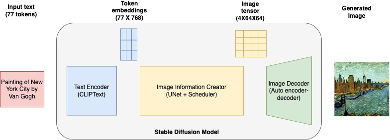
It consists of the following key elements:

• Text encoder – CLIP is a transformers-based text encoder model that takes input prompt text and converts it into token embeddings that represent each word in the text. CLIP is trained on a dataset of images and their captions, a combination of image encoder and text encoder.
• U-Net – A U-Net model takes token embeddings from CLIP along with an array of noisy inputs and produces a denoised output. This happens though a series of iterative steps, where each step processes an input latent tensor and produces a new latent space tensor that better represents the input text.
• Auto encoder-decoder – This model creates the final images. It takes the final denoised latent output from the U-Net model and converts it into images that represents the text input.

Types of Stable Diffusion models

In this post, we explore the following pre-trained Stable Diffusion models by Stability AI from the Hugging Face model hub.

stable-diffusion-2-1-base

Use this model to generate images based on a text prompt. This is a base version of the model that was trained on LAION-5B. The model was trained on a subset of the large-scale dataset LAION-5B, and mainly with English captions. We use StableDiffusionPipeline from the diffusers library to generate images from text prompts. This model can create images of dimension 512 x 512. It uses the following parameters:

• prompt – A prompt can be a text word, phrase, sentences, or paragraphs.
• negative_prompt – You can also pass a negative prompt to exclude specified elements from the image generation process and to enhance the quality of the generated images.
• guidance_scale – A higher guidance scale results in an image more closely related to the prompt, at the expense of image quality. If specified, it must be a float.

stable-diffusion-2-depth

This model is used to generate new images from existing ones while preserving the shape and depth of the objects in the original image. This stable-diffusion-2-depth model is fine-tuned from stable-diffusion-2-base, an extra input channel to process the (relative) depth prediction. We use StableDiffusionDepth2ImgPipeline from the diffusers library to load the pipeline and generate depth images. The following are the additional parameters specific to the depth model:

• image – The initial image to condition the generation of new images.
• num_inference_steps (optional) – The number of denoising steps. More denoising steps usually leads to a higher-quality image at the expense of slower inference. This parameter is modulated by strength.
• strength (optional) – Conceptually, this indicates how much to transform the reference image. The value must be between 0–1. image is used as a starting point, adding more noise to it the larger the strength. The number of denoising steps depends on the amount of noise initially added. When strength is 1, the added noise will be maximum and the denoising process will run for the full number of iterations specified in num_inference_steps. A value of 1, therefore, essentially ignores image. For more details, refer to the following code.

stable-diffusion-2-inpainting

You can use this model for AI image restoration use cases. You can also use it to create novel designs and images from the prompts and additional arguments. This model is also derived from the base model and has a mask generation strategy. It specifies the mask of the original image to represent segments to be changed and segments to leave unchanged. We use StableDiffusionUpscalePipeline from the diffusers library to apply inpaint changes on original image. The following additional parameter is specific to the depth model:

• mask_input – An image where the blacked-out portion remains unchanged during image generation and the white portion is replaced

stable-diffusion-x4-upscaler

This model is also derived from the base model, additionally trained on the 10M subset of LAION containing 2048 x 2048 images. As the name implies, it can be used to upscale lower-resolution images to higher resolutions

Use case overview

For this post, we deploy an AI image service with multiple capabilities, including generating novel images from text, changing the styles of existing images, removing unwanted objects from images, and upscaling low-resolution images to higher resolutions. Using several variations of Stable Diffusion models, you can address all of these use cases within a single SageMaker endpoint. This means that you’ll need to host large number of models in a performant, scalable, and cost-efficient way. In this post, we show how to deploy multiple Stable Diffusion models cost-effectively using SageMaker MMEs and NVIDIA Triton Inference Server. You will learn about the implementation details, optimization techniques, and best practices to work with text-to-image models.

The following table summarizes the Stable Diffusion models that we deploy to a SageMaker MME.

Solution overview

The following steps are involved in deploying Stable Diffusion models to SageMaker MMEs:

1. Use the Hugging Face hub to download the Stable Diffusion models to a local directory. This will download scheduler, text_encoder, tokenizer, unet, and vae for each Stable Diffusion model into its corresponding local directory. We use the revision="fp16" version of the model.
2. Set up the NVIDIA Triton model repository, model configurations, and model serving logic model.py. Triton uses these artifacts to serve predictions.
3. Package the conda environment with additional dependencies and the package model repository to be deployed to the SageMaker MME.
4. Package the model artifacts in an NVIDIA Triton-specific format and upload model.tar.gz to Amazon Simple Storage Service (Amazon S3). The model will be used for generating images.
5. Configure a SageMaker model, endpoint configuration, and deploy the SageMaker MME.
6. Run inference and send prompts to the SageMaker endpoint to generate images using the Stable Diffusion model. We specify the TargetModel variable and invoke different Stable Diffusion models to compare the results visually.

We have published the code to implement this solution architecture in the GitHub repo. Follow the README instructions to get started.

Serve models with an NVIDIA Triton Inference Server Python backend

We use a Triton Python backend to deploy the Stable Diffusion pipeline model to a SageMaker MME. The Python backend lets you serve models written in Python by Triton Inference Server. To use the Python backend, you need to create a Python file model.py that has the following structure: Every Python backend can implement four main functions in the TritonPythonModel class:

import triton_python_backend_utils as pb_utils
class TritonPythonModel:
"""Your Python model must use the same class name. Every Python model
that is created must have "TritonPythonModel" as the class name.
"""
def auto_complete_config(auto_complete_model_config):
def initialize(self, args):
def execute(self, requests):
def finalize(self):

Every Python backend can implement four main functions in the TritonPythonModel class: auto_complete_config, initialize, execute, and finalize.

initialize is called when the model is being loaded. Implementing initialize is optional. initialize allows you to do any necessary initializations before running inference. In the initialize function, we create a pipeline and load the pipelines using from_pretrained checkpoints. We configure schedulers from the pipeline scheduler config pipe.scheduler.config. Finally, we specify xformers optimizations to enable the xformer memory efficient parameter enable_xformers_memory_efficient_attention. We provide more details on xformers later in this post. You can refer to model.py of each model to understand the different pipeline details. This file can be found in the model repository.

The execute function is called whenever an inference request is made. Every Python model must implement the execute function. In the execute function, you are given a list of InferenceRequest objects. We pass the input text prompt to the pipeline to get an image from the model. Images are decoded and the generated image is returned from this function call.

We get the input tensor from the name defined in the model configuration config.pbtxt file. From the inference request, we get prompt, negative_prompt, and gen_args, and decode them. We pass all the arguments to the model pipeline object. Encode the image to return the generated image predictions. You can refer to the config.pbtxt file of each model to understand the different pipeline details. This file can be found in the model repository. Finally, we wrap the generated image in InferenceResponse and return the response.

Implementing finalize is optional. This function allows you to do any cleanups necessary before the model is unloaded from Triton Inference Server.

When working with the Python backend, it’s the user’s responsibility to ensure that the inputs are processed in a batched manner and that responses are sent back accordingly. To achieve this, we recommend following these steps:

1. Loop through all requests in the requests object to form a batched_input.
2. Run inference on the batched_input.
3. Split the results into multiple InferenceResponse objects and concatenate them as the responses.

Refer to the Triton Python backend documentation or Host ML models on Amazon SageMaker using Triton: Python backend for more details.

NVIDIA Triton model repository and configuration

The model repository contains the model serving script, model artifacts and tokenizer artifacts, a packaged conda environment (with dependencies needed for inference), the Triton config file, and the Python script used for inference. The latter is mandatory when you use the Python backend, and you should use the Python file model.py. Let’s explore the configuration file of the inpaint Stable Diffusion model and understand the different options specified:

name: "sd_inpaint"
backend: "python"
max_batch_size: 8
input [
  {
    name: "prompt"
    data_type: TYPE_STRING
    dims: [
      -1
    ]
  },
  {
    name: "negative_prompt"
    data_type: TYPE_STRING
    dims: [
      -1
    ]
    optional: true
  },
  {
    name: "image"
    data_type: TYPE_STRING
    dims: [
      -1
    ]
  },
  {
    name: "mask_image"
    data_type: TYPE_STRING
    dims: [
      -1
    ]
  },
  {
    name: "gen_args"
    data_type: TYPE_STRING
    dims: [
      -1
    ]
    optional: true
  }
]
output [
  {
    name: "generated_image"
    data_type: TYPE_STRING    
    dims: [
      -1
    ]
  }
]
instance_group [
  {
    kind: KIND_GPU
  }
]
parameters: {
  key: "EXECUTION_ENV_PATH",
  value: {string_value: "/tmp/conda/sd_env.tar.gz"
  }
}

The following table explains the various parameters and values:

For details about the model repository and configurations of other Stable Diffusion models, refer to the code in the GitHub repo. Each directory contains artifacts for the specific Stable Diffusion models.

Package a conda environment and extend the SageMaker Triton container

SageMaker NVIDIA Triton container images don’t contain libraries like transformer, accelerate, and diffusers to deploy and serve Stable Diffusion models. However, Triton allows you to bring additional dependencies using conda-pack. Let’s start by creating the conda environment with the necessary dependencies outlined in the environment.yml file and create a tar model artifact sd_env.tar.gz file containing the conda environment with dependencies installed in it. Run the following YML file to create a conda-pack artifact and copy the artifact to the local directory from where it will be uploaded to Amazon S3. Note that we will be uploading the conda artifacts as one of the models in the MME and invoking this model to set up the conda environment in the SageMaker hosting ML instance.

%%writefile environment.yml
name: mme_env
dependencies:
  - python=3.8
  - pip
  - pip:
      - numpy
      - torch --extra-index-url https://download.pytorch.org/whl/cu118
      - accelerate
      - transformers
      - diffusers
      - xformers
      - conda-pack

!conda env create -f environment.yml –force

Upload model artifacts to Amazon S3

SageMaker expects the .tar.gz file containing each Triton model repository to be hosted on the multi-model endpoint. Therefore, we create a tar artifact with content from the Triton model repository. We can use this S3 bucket to host thousands of model artifacts, and the SageMaker MME will use models from this location to dynamically load and serve a large number of models. We store all the Stable Diffusion models in this Amazon S3 location.

Deploy the SageMaker MME

In this section, we walk through the steps to deploy the SageMaker MME by defining container specification, SageMaker model and endpoint configurations.

Define the serving container

In the container definition, define the ModelDataUrl to specify the S3 directory that contains all the models that the SageMaker MME will use to load and serve predictions. Set Mode to MultiModel to indicate that SageMaker will create the endpoint with the MME container specifications. We set the container with an image that supports deploying MMEs with GPU. See Supported algorithms, frameworks, and instances for more details.

We see all three model artifacts in the following Amazon S3 ModelDataUrl location:

container = {"Image": mme_triton_image_uri, 
             "ModelDataUrl": model_data_url, 
             "Mode": "MultiModel"}

Create an MME object

We use the SageMaker Boto3 client to create the model using the create_model API. We pass the container definition to the create model API along with ModelName and ExecutionRoleArn:

create_model_response = sm_client.create_model(
    ModelName=sm_model_name, 
    ExecutionRoleArn=role, 
    PrimaryContainer=container
)

Define configurations for the MME

Create an MME configuration using the create_endpoint_config Boto3 API. Specify an accelerated GPU computing instance in InstanceType (we use the same instance type that we are using to host our SageMaker notebook). We recommend configuring your endpoints with at least two instances with real-life use cases. This allows SageMaker to provide a highly available set of predictions across multiple Availability Zones for the models.

create_endpoint_config_response = sm_client.create_endpoint_config(
    EndpointConfigName=endpoint_config_name,
    ProductionVariants=[
        {
            "InstanceType": instance_type,
            "InitialVariantWeight": 1,
            "InitialInstanceCount": 1,
            "ModelName": sm_model_name,
            "VariantName": "AllTraffic",
        }
    ],
)

Create an MME

Use the preceding endpoint configuration to create a new SageMaker endpoint and wait for the deployment to finish:

create_endpoint_response = sm_client.create_endpoint(
                EndpointName=endpoint_name, 
                EndpointConfigName=endpoint_config_name
)

The status will change to InService when the deployment is successful.

Generate images using different versions of Stable Diffusion models

Let’s start by invoking the base model with a prompt and getting the generated image. We pass the inputs to the base model with prompt, negative_prompt, and gen_args as a dictionary. We set the data type and shape of each input item in the dictionary and pass it as input to the model.

inputs = dict(prompt = "Infinity pool on top of a high rise overlooking Central Park",
             negative_prompt = "blur,low detail, low quality",
             gen_args = json.dumps(dict(num_inference_steps=50, guidance_scale=8))
)
payload = {
    "inputs":
        [{"name": name, "shape": [1,1], "datatype": "BYTES", "data": [data]} for name, data in inputs.items()]
}
response = runtime_sm_client.invoke_endpoint(
        EndpointName=endpoint_name,
        ContentType="application/octet-stream",
        Body=json.dumps(payload),
        TargetModel="sd_base.tar.gz", 
    )
output = json.loads(response["Body"].read().decode("utf8"))["outputs"]
decode_image(output[0]["data"][0])

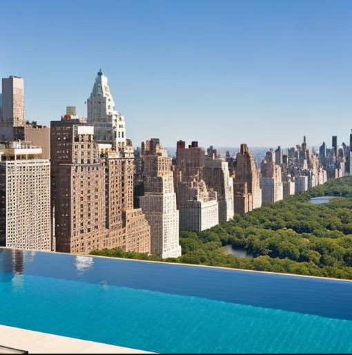
Prompt: Infinity pool on top of a high rise overlooking Central Park

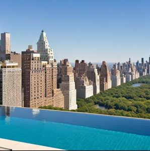
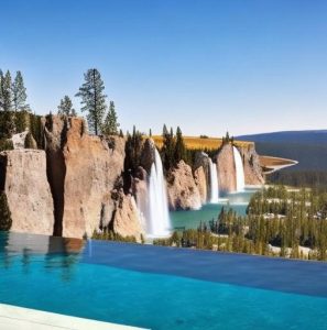
Working with this image, we can modify it with the versatile Stable Diffusion depth model. For example, we can change the style of the image to an oil painting, or change the setting from Central Park to Yellowstone National Park simply by passing the original image along with a prompt describing the changes we would like to see.

We invoke the depth model by specifying sd_depth.tar.gz in the TargetModel of the invoke_endpoint function call. In the outputs, notice how the orientation of the original image is preserved, but for one example, the NYC buildings have been transformed into rock formations of the same shape.

inputs = dict(prompt = "highly detailed oil painting of an inifinity pool overlooking central park",
              image=image,
              gen_args = json.dumps(dict(num_inference_steps=50, strength=0.9))
              )
payload = {
    "inputs":
        [{"name": name, "shape": [1,1], "datatype": "BYTES", "data": [data]} for name, data in inputs.items()]
}
response = runtime_sm_client.invoke_endpoint(
        EndpointName=endpoint_name,
        ContentType="application/octet-stream",
        Body=json.dumps(payload),
        TargetModel="sd_depth.tar.gz", 
    )
output = json.loads(response["Body"].read().decode("utf8"))["outputs"]
print("original image")
display(original_image)
print("generated image")
display(decode_image(output[0]["data"][0]))

Original image	Oil painting	Yellowstone Park

Another useful model is Stable Diffusion inpainting, which we can use to remove certain parts of the image. Let’s say you want to remove the tree in the following example image. We can do so by invoking the inpaint model sd_inpaint.tar.gz. To remove the tree, we need to pass a mask_image, which indicates which regions of the image should be retained and which should be filled in. The black pixel portion of the mask image indicates the regions that should remain unchanged, and the white pixels indicate what should be replaced.

image = encode_image(original_image).decode("utf8")
mask_image = encode_image(Image.open("sample_images/bertrand-gabioud-mask.png")).decode("utf8")
inputs = dict(prompt = "building, facade, paint, windows",
              image=image,
              mask_image=mask_image,
              negative_prompt = "tree, obstruction, sky, clouds",
              gen_args = json.dumps(dict(num_inference_steps=50, guidance_scale=10))
              )
payload = {
    "inputs":
        [{"name": name, "shape": [1,1], "datatype": "BYTES", "data": [data]} for name, data in inputs.items()]
}
response = runtime_sm_client.invoke_endpoint(
        EndpointName=endpoint_name,
        ContentType="application/octet-stream",
        Body=json.dumps(payload),
        TargetModel="sd_inpaint.tar.gz", 
    )
output = json.loads(response["Body"].read().decode("utf8"))["outputs"]
decode_image(output[0]["data"][0])

Original image	Mask image	Inpaint image

In our final example, we downsize the original image that was generated earlier from its 512 x 512 resolution to 128 x 128. We then invoke the Stable Diffusion upscaler model to upscale the image back to 512 x 512. We use the same prompt to upscale the image as what we used to generate the initial image. While not necessary, providing a prompt that describes the image helps guide the upscaling process and should lead to better results.

low_res_image = output_image.resize((128, 128))
inputs = dict(prompt = "Infinity pool on top of a high rise overlooking Central Park",
             image=encode_image(low_res_image).decode("utf8")
)

payload = {
    "inputs":
        [{"name": name, "shape": [1,1], "datatype": "BYTES", "data": [data]} for name, data in inputs.items()]
}

response = runtime_sm_client.invoke_endpoint(
        EndpointName=endpoint_name,
        ContentType="application/octet-stream",
        Body=json.dumps(payload),
        TargetModel="sd_upscale.tar.gz", 
    )
output = json.loads(response["Body"].read().decode("utf8"))["outputs"]
upscaled_image = decode_image(output[0]["data"][0])

Low-resolution image	Upscaled image

Although the upscaled image is not as detailed as the original, it’s a marked improvement over the low-resolution one.

Optimize for memory and speed

The xformers library is a way to speed up image generation. This optimization is only available for NVIDIA GPUs. It speeds up image generation and lowers VRAM usage. We have used the xformers library for memory-efficient attention and speed. When the enable_xformers_memory_efficient_attention option is enabled, you should observe lower GPU memory usage and a potential speedup at inference time.

Clean Up

Follow the instruction in the clean up section of the notebook to delete the resource provisioned part of this blog to avoid unnecessary charges. Refer Amazon SageMaker Pricing for details the cost of the inference instances.

Conclusion

In this post, we discussed Stable Diffusion models and how you can deploy different versions of Stable Diffusion models cost-effectively using SageMaker multi-model endpoints. You can use this approach to build a creator image generation and editing tool. Check out the code samples in the GitHub repo to get started and let us know about the cool generative AI tool that you build.

About the Authors

Simon Zamarin is an AI/ML Solutions Architect whose main focus is helping customers extract value from their data assets. In his spare time, Simon enjoys spending time with family, reading sci-fi, and working on various DIY house projects.

Vikram Elango is a Sr. AI/ML Specialist Solutions Architect at AWS, based in Virginia, US. He is currently focused on generative AI, LLMs, prompt engineering, large model inference optimization, and scaling ML across enterprises. Vikram helps financial and insurance industry customers with design and architecture to build and deploy ML applications at scale. In his spare time, he enjoys traveling, hiking, cooking, and camping with his family.

João Moura is an AI/ML Specialist Solutions Architect at AWS, based in Spain. He helps customers with deep learning model training and inference optimization, and more broadly building large-scale ML platforms on AWS. He is also an active proponent of ML-specialized hardware and low-code ML solutions.

Saurabh Trikande is a Senior Product Manager for Amazon SageMaker Inference. He is passionate about working with customers and is motivated by the goal of democratizing machine learning. He focuses on core challenges related to deploying complex ML applications, multi-tenant ML models, cost optimizations, and making deployment of deep learning models more accessible. In his spare time, Saurabh enjoys hiking, learning about innovative technologies, following TechCrunch, and spending time with his family.

Read More

One of the most common applications of generative AI and large language models (LLMs) in an enterprise environment is answering questions based on the enterprise’s knowledge corpus. Amazon Lex provides the framework for building AI based chatbots. Pre-trained foundation models (FMs) perform well at natural language understanding (NLU) tasks such summarization, text generation and question answering on a broad variety of topics but either struggle to provide accurate (without hallucinations) answers or completely fail at answering questions about content that they haven’t seen as part of their training data. Furthermore, FMs are trained with a point in time snapshot of data and have no inherent ability to access fresh data at inference time; without this ability they might provide responses that are potentially incorrect or inadequate.

A commonly used approach to address this problem is to use a technique called Retrieval Augmented Generation (RAG). In the RAG-based approach we convert the user question into vector embeddings using an LLM and then do a similarity search for these embeddings in a pre-populated vector database holding the embeddings for the enterprise knowledge corpus. A small number of similar documents (typically three) is added as context along with the user question to the “prompt” provided to another LLM and then that LLM generates an answer to the user question using information provided as context in the prompt. RAG models were introduced by Lewis et al. in 2020 as a model where parametric memory is a pre-trained seq2seq model and the non-parametric memory is a dense vector index of Wikipedia, accessed with a pre-trained neural retriever. To understand the overall structure of a RAG-based approach, refer to Question answering using Retrieval Augmented Generation with foundation models in Amazon SageMaker JumpStart.

In this post we provide a step-by-step guide with all the building blocks for creating an enterprise ready RAG application such as a question answering bot. We use a combination of different AWS services, open-source foundation models (FLAN-T5 XXL for text generation and GPT-j-6B for embeddings) and packages such as LangChain for interfacing with all the components and Streamlit for building the bot frontend.

We provide an AWS Cloud Formation template to stand up all the resources required for building this solution. We then demonstrate how to use LangChain for tying everything together:

• Interfacing with LLMs hosted on Amazon SageMaker.
• Chunking of knowledge base documents.
• Ingesting document embeddings into Amazon OpenSearch Service.
• Implementing the question answering task.

We can use the same architecture to swap the open-source models with the Amazon Titan models. After Amazon Bedrock launches, we will publish a follow-up post showing how to implement similar generative AI applications using Amazon Bedrock, so stay tuned.

Solution overview

We use the SageMaker docs as the knowledge corpus for this post. We convert the HTML pages on this site into smaller overlapping chunks (to retain some context continuity between chunks) of information and then convert these chunks into embeddings using the gpt-j-6b model and store the embeddings in OpenSearch Service. We implement the RAG functionality inside an AWS Lambda function with Amazon API Gateway to handle routing all requests to the Lambda. We implement a chatbot application in Streamlit which invokes the function via the API Gateway and the function does a similarity search in the OpenSearch Service index for the embeddings of user question. The matching documents (chunks) are added to the prompt as context by the Lambda function and then the function uses the flan-t5-xxl model deployed as a SageMaker endpoint to generate an answer to the user question. All the code for this post is available in the GitHub repo.

The following figure represents the high-level architecture of the proposed solution.

Figure 1: Architecture

Step-by-step explanation:

1. The User provides a question via the Streamlit web application.
2. The Streamlit application invokes the API Gateway endpoint REST API.
3. The API Gateway invokes the Lambda function.
4. The function invokes the SageMaker endpoint to convert user question into embeddings.
5. The function invokes invokes an OpenSearch Service API to find similar documents to the user question.
6. The function creates a “prompt” with the user query and the “similar documents” as context and asks the SageMaker endpoint to generate a response.
7. The response is provided from the function to the API Gateway.
8. The API Gateway provides the response to the Streamlit application.
9. The User is able to view the response on the Streamlit application,

As illustrated in the architecture diagram, we use the following AWS services:

• SageMaker and Amazon SageMaker JumpStart for hosting the two LLMs.
• OpenSearch Service for storing the embeddings of the enterprise knowledge corpus and doing similarity search with user questions.
• Lambda for implementing the RAG functionality and exposing it as a REST endpoint via the API Gateway.
• Amazon SageMaker Processing jobs for large scale data ingestion into OpenSearch.
• Amazon SageMaker Studio for hosting the Streamlit application.
• AWS Identity and Access Management roles and policies for access management.
• AWS CloudFormation for creating the entire solution stack through infrastructure as code.

In terms of open-source packages used in this solution, we use LangChain for interfacing with OpenSearch Service and SageMaker, and FastAPI for implementing the REST API interface in the Lambda.

The workflow for instantiating the solution presented in this post in your own AWS account is as follows:

1. Run the CloudFormation template provided with this post in your account. This will create all the necessary infrastructure resources needed for this solution:
   • SageMaker endpoints for the LLMs
   • OpenSearch Service cluster
   • API Gateway
   • Lambda function
   • SageMaker Notebook
   • IAM roles
2. Run the data_ingestion_to_vectordb.ipynb notebook in the SageMaker notebook to ingest data from SageMaker docs into an OpenSearch Service index.
3. Run the Streamlit application on a terminal in Studio and open the URL for the application in a new browser tab.
4. Ask your questions about SageMaker via the chat interface provided by the Streamlit app and view the responses generated by the LLM.

These steps are discussed in detail in the following sections.

Prerequisites

To implement the solution provided in this post, you should have an AWS account and familiarity with LLMs, OpenSearch Service and SageMaker.

We need access to accelerated instances (GPUs) for hosting the LLMs. This solution uses one instance each of ml.g5.12xlarge and ml.g5.24xlarge; you can check the availability of these instances in your AWS account and request these instances as needed via a Sevice Quota increase request as shown in the following screenshot.

Figure 2: Service Quota Increase Request

Use AWS Cloud Formation to create the solution stack

We use AWS CloudFormation to create a SageMaker notebook called aws-llm-apps-blog and an IAM role called LLMAppsBlogIAMRole. Choose Launch Stack for the Region you want to deploy resources to. All parameters needed by the CloudFormation template have default values already filled in, except for the OpenSearch Service password which you’d have to provide. Make a note of the OpenSearch Service username and password, we use those in subsequent steps. This template takes about 15 minutes to complete.

AWS Region	Link
us-east-1
us-west-2
eu-west-1
ap-northeast-1

After the stack is created successfully, navigate to the stack’s Outputs tab on the AWS CloudFormation console and note the values for OpenSearchDomainEndpoint and LLMAppAPIEndpoint. We use those in the subsequent steps.

Figure 3: Cloud Formation Stack Outputs

Ingest the data into OpenSearch Service

To ingest the data, complete the following steps:

1. On the SageMaker console, choose Notebooks in the navigation pane.
2. Select the notebook aws-llm-apps-blog and choose Open JupyterLab.
   

   Figure 4: Open JupyterLab

3. Choose data_ingestion_to_vectordb.ipynb to open it in JupyterLab. This notebook will ingest the SageMaker docs to an OpenSearch Service index called llm_apps_workshop_embeddings.
   

   Figure 5: Open Data Ingestion Notebook

4. When the notebook is open, on the Run menu, choose Run All Cells to run the code in this notebook. This will download the dataset locally into the notebook and then ingest it into the OpenSearch Service index. This notebook takes about 20 minutes to run. The notebook also ingests the data into another vector database called FAISS. The FAISS index files are saved locally and the uploaded to Amazon Simple Storage Service (S3) so that they can optionally be used by the Lambda function as an illustration of using an alternate vector database.
   

   Figure 6: Notebook Run All Cells

Now we’re ready to split the documents into chunks, which can then be converted into embeddings to be ingested into OpenSearch. We use the LangChain RecursiveCharacterTextSplitter class to chunk the documents and then use the LangChain SagemakerEndpointEmbeddingsJumpStart class to convert these chunks into embeddings using the gpt-j-6b LLM. We store the embeddings in OpenSearch Service via the LangChain OpenSearchVectorSearch class. We package this code into Python scripts that are provided to the SageMaker Processing Job via a custom container. See the data_ingestion_to_vectordb.ipynb notebook for the full code.

5. Create a custom container, then install in it the LangChain and opensearch-py Python packages.
6. Upload this container image to Amazon Elastic Container Registry (ECR).
7. We use the SageMaker ScriptProcessor class to create a SageMaker Processing job that will run on multiple nodes.
   • The data files available in Amazon S3 are automatically distributed across in the SageMaker Processing job instances by setting s3_data_distribution_type='ShardedByS3Key' as part of the ProcessingInput provided to the processing job.
   • Each node processes a subset of the files and this brings down the overall time required to ingest the data into OpenSearch Service.
   • Each node also uses Python multiprocessing to internally also parallelize the file processing. Therefore, there are two levels of parallelization happening, one at the cluster level where individual nodes are distributing the work (files) amongst themselves and another at the node level where the files in a node are also split between multiple processes running on the node.

      # setup the ScriptProcessor with the above parameters
     processor = ScriptProcessor(base_job_name=base_job_name,
                                 image_uri=image_uri,
                                 role=aws_role,
                                 instance_type=instance_type,
                                 instance_count=instance_count,
                                 command=["python3"],
                                 tags=tags)
     
     # setup input from S3, note the ShardedByS3Key, this ensures that 
     # each instance gets a random and equal subset of the files in S3.
     inputs = [ProcessingInput(source=f"s3://{bucket}/{app_name}/{DOMAIN}",
                               destination='/opt/ml/processing/input_data',
                               s3_data_distribution_type='ShardedByS3Key',
                               s3_data_type='S3Prefix')]
     
     
     logger.info(f"creating an opensearch index with name={opensearch_index}")
     # ready to run the processing job
     st = time.time()
     processor.run(code="container/load_data_into_opensearch.py",
                   inputs=inputs,
                   outputs=[],
                   arguments=["--opensearch-cluster-domain", opensearch_domain_endpoint,
                             "--opensearch-secretid", os_creds_secretid_in_secrets_manager,
                             "--opensearch-index-name", opensearch_index,
                             "--aws-region", aws_region,
                             "--embeddings-model-endpoint-name", embeddings_model_endpoint_name,
                             "--chunk-size-for-doc-split", str(CHUNK_SIZE_FOR_DOC_SPLIT),
                             "--chunk-overlap-for-doc-split", str(CHUNK_OVERLAP_FOR_DOC_SPLIT),
                             "--input-data-dir", "/opt/ml/processing/input_data",
                             "--create-index-hint-file", CREATE_OS_INDEX_HINT_FILE,
                             "--process-count", "2"])

8. Close the notebook after all cells run without any error. Your data is now available in OpenSearch Service. Enter the following URL in your browser’s address bar to get a count of documents in the llm_apps_workshop_embeddings index. Use the OpenSearch Service domain endpoint from the CloudFormation stack outputs in the URL below. You’d be prompted for the OpenSearch Service username and password, these are available from the CloudFormations stack.

   https://your-opensearch-domain-endpoint/llm_apps_workshop_embeddings/_count

The browser window should show an output similar to the following. This output shows that 5,667 documents were ingested into the llm_apps_workshop_embeddings index. {"count":5667,"_shards":{"total":5,"successful":5,"skipped":0,"failed":0}}

Run the Streamlit application in Studio

Now we’re ready to run the Streamlit web application for our question answering bot. This application allows the user to ask a question and then fetches the answer via the /llm/rag REST API endpoint provided by the Lambda function.

Studio provides a convenient platform to host the Streamlit web application. The following steps describes how to run the Streamlit app on Studio. Alternatively, you could also follow the same procedure to run the app on your laptop.

1. Open Studio and then open a new terminal.
2. Run the following commands on the terminal to clone the code repository for this post and install the Python packages needed by the application:

   git clone https://github.com/aws-samples/llm-apps-workshop
   cd llm-apps-workshop/blogs/rag/app
   pip install -r requirements.txt

3. The API Gateway endpoint URL that is available from the CloudFormation stack output needs to be set in the webapp.py file. This is done by running the following sed command. Replace the replace-with-LLMAppAPIEndpoint-value-from-cloudformation-stack-outputs in the shell commands with the value of the LLMAppAPIEndpoint field from the CloudFormation stack output and then run the following commands to start a Streamlit app on Studio.

   
   EP=replace-with-LLMAppAPIEndpoint-value-from-cloudformation-stack-outputs
   # replace __API_GW_ENDPOINT__ with  output from the cloud formation stack
   sed -i "s|__API_GW_ENDPOINT__|$EP|g" webapp.py
   streamlit run webapp.py

4. When the application runs successfully, you’ll see an output similar to the following (the IP addresses you will see will be different from the ones shown in this example). Note the port number (typically 8501) from the output to use as part of the URL for app in the next step.

   sagemaker-user@studio$ streamlit run webapp.py 
   
   Collecting usage statistics. To deactivate, set browser.gatherUsageStats to False.
   
   You can now view your Streamlit app in your browser.
   
   Network URL: http://169.255.255.2:8501
   External URL: http://52.4.240.77:8501

5. You can access the app in a new browser tab using a URL that is similar to your Studio domain URL. For example, if your Studio URL is https://d-randomidentifier.studio.us-east-1.sagemaker.aws/jupyter/default/lab? then the URL for your Streamlit app will be https://d-randomidentifier.studio.us-east-1.sagemaker.aws/jupyter/default/proxy/8501/webapp (notice that lab is replaced with proxy/8501/webapp). If the port number noted in the previous step is different from 8501 then use that instead of 8501 in the URL for the Streamlit app.

The following screenshot shows the app with a couple of user questions.

A closer look at the RAG implementation in the Lambda function

Now that we have the application working end to end, lets take a closer look at the Lambda function. The Lambda function uses FastAPI to implement the REST API for RAG and the Mangum package to wrap the API with a handler that we package and deploy in the function. We use the API Gateway to route all incoming requests to invoke the function and handle the routing internally within our application.

The following code snippet shows how we find documents in the OpenSearch index that are similar to the user question and then create a prompt by combining the question and the similar documents. This prompt is then provided to the LLM for generating an answer to the user question.

@router.post("/rag")
async def rag_handler(req: Request) -> Dict[str, Any]:
    # dump the received request for debugging purposes
    logger.info(f"req={req}")

    # initialize vector db and SageMaker Endpoint
    _init(req)

    # Use the vector db to find similar documents to the query
    # the vector db call would automatically convert the query text
    # into embeddings
    docs = _vector_db.similarity_search(req.q, k=req.max_matching_docs)
    logger.info(f"here are the {req.max_matching_docs} closest matching docs to the query="{req.q}"")
    for d in docs:
        logger.info(f"---------")
        logger.info(d)
        logger.info(f"---------")

    # now that we have the matching docs, lets pack them as a context
    # into the prompt and ask the LLM to generate a response
    prompt_template = """Answer based on context:nn{context}nn{question}"""

    prompt = PromptTemplate(
        template=prompt_template, input_variables=["context", "question"]
    )
    logger.info(f"prompt sent to llm = "{prompt}"")
    chain = load_qa_chain(llm=_sm_llm, prompt=prompt)
    answer = chain({"input_documents": docs, "question": req.q}, return_only_outputs=True)['output_text']
    logger.info(f"answer received from llm,nquestion: "{req.q}"nanswer: "{answer}"")
    resp = {'question': req.q, 'answer': answer}
    if req.verbose is True:
        resp['docs'] = docs

    return resp

Clean up

To avoid incurring future charges, delete the resources. You can do this by deleting the CloudFormation stack as shown in the following screenshot.

Figure 7: Cleaning Up

Conclusion

In this post, we showed how to create an enterprise ready RAG solution using a combination of AWS service, open-source LLMs and open-source Python packages.

We encourage you to learn more by exploring JumpStart, Amazon Titan models, Amazon Bedrock, and OpenSearch Service and building a solution using the sample implementation provided in this post and a dataset relevant to your business. If you have questions or suggestions, leave a comment.

About the Authors

Amit Arora is an AI and ML Specialist Architect at Amazon Web Services, helping enterprise customers use cloud-based machine learning services to rapidly scale their innovations. He is also an adjunct lecturer in the MS data science and analytics program at Georgetown University in Washington D.C.

Dr. Xin Huang is a Senior Applied Scientist for Amazon SageMaker JumpStart and Amazon SageMaker built-in algorithms. He focuses on developing scalable machine learning algorithms. His research interests are in the area of natural language processing, explainable deep learning on tabular data, and robust analysis of non-parametric space-time clustering. He has published many papers in ACL, ICDM, KDD conferences, and Royal Statistical Society: Series A.

Navneet Tuteja is a Data Specialist at Amazon Web Services. Before joining AWS, Navneet worked as a facilitator for organizations seeking to modernize their data architectures and implement comprehensive AI/ML solutions. She holds an engineering degree from Thapar University, as well as a master’s degree in statistics from Texas A&M University.

Read More