Text-to-image/video models like Midjourney, Imagen3, Stable Diffusion, and Sora can generate aesthetic, photo-realistic visuals from natural language prompts, for example, given “Several giant woolly mammoths approach, treading through a snowy meadow…”, Sora generates:
But how do we know if these models generate what we desire? For example, if the prompt is “The brown dog chases the black dog around a tree”, how can we tell if the model shows the dogs “chasing around a tree” rather than “playing in a backyard”? More generally, how should we evaluate these generative models? While humans can easily judge whether a generated image aligns with a prompt, large-scale human evaluation is costly. To address this, we introduce a new evaluation metric (VQAScore) and benchmark dataset (GenAI-Bench) [Lin et al., ECCV 2024] for automated evaluation of text-to-visual generative models. Our evaluation framework was recently employed by Google Deepmind to evaluate their Imagen3 model!
We introduce VQAScore[Lin et al., ECCV 2024] —a simple yet powerful metric to evaluate state-of-the-art generative models such as DALL-E 3, Midjourney, and Stable Diffusion (SD-XL). VQAScore aligns more closely with human judgments and significantly outperforms the popular CLIPScore [Hessel et al., 2021] on challenging compositional prompts collected from professional designers in our GenAI-Bench [Li et al., CVPR 2024].
Background
While state-of-the-art text-to-visual models perform well on simple prompts, they struggle with complex prompts which involve multiple objects and require higher-order reasoning like negation. Recent models like DALL-E 3 [Betker et al., OpenAI 2023] and Stable Diffusion [Esser et al., Stability AI 2024] address this by training on higher-quality image-text pairs (often using language models such as GPT-4 to rewrite captions) or using strong language encoders like T5 [Raffel et al., JMLR 2020].
As text-to-visual models advance, evaluating them has become a challenging task. To measure similarity between two images, perceptual metrics like Learned Perceptual Image Patch Similarity (LPIPS) [Zhang et al., CVPR 2018] uses a pre-trained image encoder to embed and compare image features, with higher similarity indicating the images look alike. For measuring similarity between a text prompt and an image (image-text alignment), the common practice is to rely on OpenAI’s pre-trained CLIP model [Radford et al., OpenAI 2021]. CLIP includes both an image encoder and a text encoder, trained on millions of image-text pairs, to embed images and texts into the same feature space, where higher similarity suggests stronger image-text alignment. This approach is commonly referred to as CLIPScore [Hessel et al., EMNLP 2021].
Previous evaluation metrics for generative models: Perceptual metrics like LPIPS use a pre-trained image encoder to embed the original and reconstructed images into two 1D vectors, and then compute their distance. As a result, perceptually similar images will have a higher LPIPS score. On the other hand, CLIPScore uses the dual encoders of a pre-trained CLIP model to embed images and texts into the same space, where semantically aligned pairs will have a higher CLIPScore.
However, CLIPScore suffers from a notorious “bag-of-words” issue. This means that when embedding texts, CLIP can ignore word order, leading to mistakes like confusing “The moon is over the cow” with “The cow is over the moon”.
Examples from the challenging image-text matching benchmark Winoground [Thrush et al., CVPR 2022], where CLIPScore often assigns higher scores to incorrect image-text pairs. In general, CLIPScore struggles with multiple objects, attribute bindings, object relationships, and complex numerical (counting) and logical reasoning. In contrast, our VQAScore excels in these challenging scenarios.
Why is CLIPScore limited? Our prior work [Lin et al., ICML 2024], along with others [Yuksekgonul et al., ICLR 2023], suggests its bottleneck lies in its discriminative training approach. The structure of CLIP’s loss function causes it to maximize similarity between an image and its caption and minimize similarity between an image and a small set of unrelated captions. However, this structure allows for shortcut — CLIP often minimizes similarity to negatives by simply recognizing main objects, ignoring finer details. In contrast, we suspect that generative vision-language models trained for image-to-text generation (e.g., image captioning) are more robust because they cannot rely on shortcuts—generating the correct text sequence requires a precise understanding of word order.
VQAScore: A Strong and Simple Text-to-Visual Metric
Based on generative vision-language models trained for visual-question-answering (VQA) tasks that generate an answer from an image and a question, we propose a simple metric, VQAScore. Given an image and a text prompt, we define their alignment as the probability of the model responding “Yes” to the question, “Does this image show ‘{text}’? Please answer yes or no.” For example, given an image and the text prompt “the cow over the moon”, we would compute the following probability:
(P(“Yes” | image, “Does this figure show ‘the cow over the moon’? Please answer yes or no.”) )
VQAScore is calculated as the probability of a visual-question-answering (VQA) model responding “Yes” to a simple yes-or-no question like, “Does this figure show [prompt]? Please answer yes or no.” VQAScore can be implemented in most VQA models trained with next-token prediction loss, where the model predicts the next token based on the current tokens. This figure illustrates the implementation of VQAScore: on the left, the image and question are tokenized and fed into an image-question encoder; on the right, an answer decoder calculates the probability of the next answer token (i.e., “Yes”) auto-regressively based on the output tokens from the image-question encoder.
Our paper [Lin et al., ECCV 2024] shows that VQAScore outperforms CLIPScore and all other evaluation metrics across benchmarks measuring correlation with human judgements on image-text alignment, including Winoground [Thrush et al., CVPR 2022], TIFA160 [Hu et al., ICCV 2023], Pick-a-pic [Kirstain et al., NeurIPS 2023]. VQAScore even outperforms metrics that use additional fine-tuning data or proprietary models like GPT-4 (Vision). These metrics can be grouped into three types:
(1) Human-feedback approaches, like ImageReward, PickScore, and Human Preference Score, fine-tune CLIP using human ratings of generated images. (2) LLM-as-a-judge approaches, like VIEScore, use LLMs such as GPT-4 (Vision) to directly output image-text alignment scores, e.g., asking the model to output a score between 0 to 100. (3) Divide-and-conquer approaches like TIFA, Davidsonian, and Gecko decompose text prompts into simpler question-answer pairs (often using LLMs like GPT-4) and then use VQA models to assess alignment based on answer accuracy.
Compared to these metrics, VQAScore offers several key advantages:
(1) No fine-tuning: VQAScore performs well using off-the-shelf VQA models without the need for fine-tuning on human feedback. (2) Token probabilityis more precise than text generation: LLM-as-a-judge methods often assign similar and random scores (like 90) to most image-text pairs, regardless of alignment. (3) No prompt decomposition: While divide-and-conquer approaches may seem promising, prompt decomposition is error-prone. For example, with the prompt “someone talks on the phone happily while another person sits angrily,” the state-of-the-art method Davidsonian wrongly asks irrelevant questions such as, “Is there another person?”
In addition, our paper also demonstrates VQAScore’s preliminary success in evaluating text-to-video and 3D generation. We are encouraged by recent work like Generative Verifier, which supports a similar approach for evaluating language models. Finally, DeepMind’s Imagen3 suggests that stronger models like Gemini could further enhance VQAScore, indicating that it scales well with future image-to-text models.
GenAI-Bench: A Compositional Text-to-Visual Generation Benchmark
During our studies, we found that previous text-to-visual benchmarks like COCO and PartiPrompt lacked sufficiently challenging prompts. To address this, we collected 1,600 real prompts from graphic designers using tools like Midjourney. This results in GenAI-Bench [Li et al., CVPR 2024], which covers a broader range of compositional reasoning and presents a tougher challenge to text-to-visual models.
GenAI-Bench [Li et al., CVPR 2024] reflects how users seek precise control in text-to-visual generation using compositional prompts. For example, users often add details by specifying compositions of objects, scenes, attributes, and relationships (spatial/action/part). Additionally, user prompts may involve higher-order reasoning, including counting, comparison, differentiation, and logic (negation/universality).
After gathering these diverse, real-world prompts, we collected 1-to-5 Likert-scale ratings on the generated images from state-of-the-art models like Midjourney and Stable Diffusion, with three annotators evaluating each image-text pair. We also discuss in the paper how these human ratings can be used to better evaluate future automated metrics.
We collect prompts from professional designers to ensure GenAI-Bench reflects real-world needs. Designers write prompts on general topics (e.g., food, animals, household objects) without copyrighted characters or celebrities. We carefully tag each prompt with its evaluated skills and hire human annotators to rate images and videos generated by state-of-the-art models.
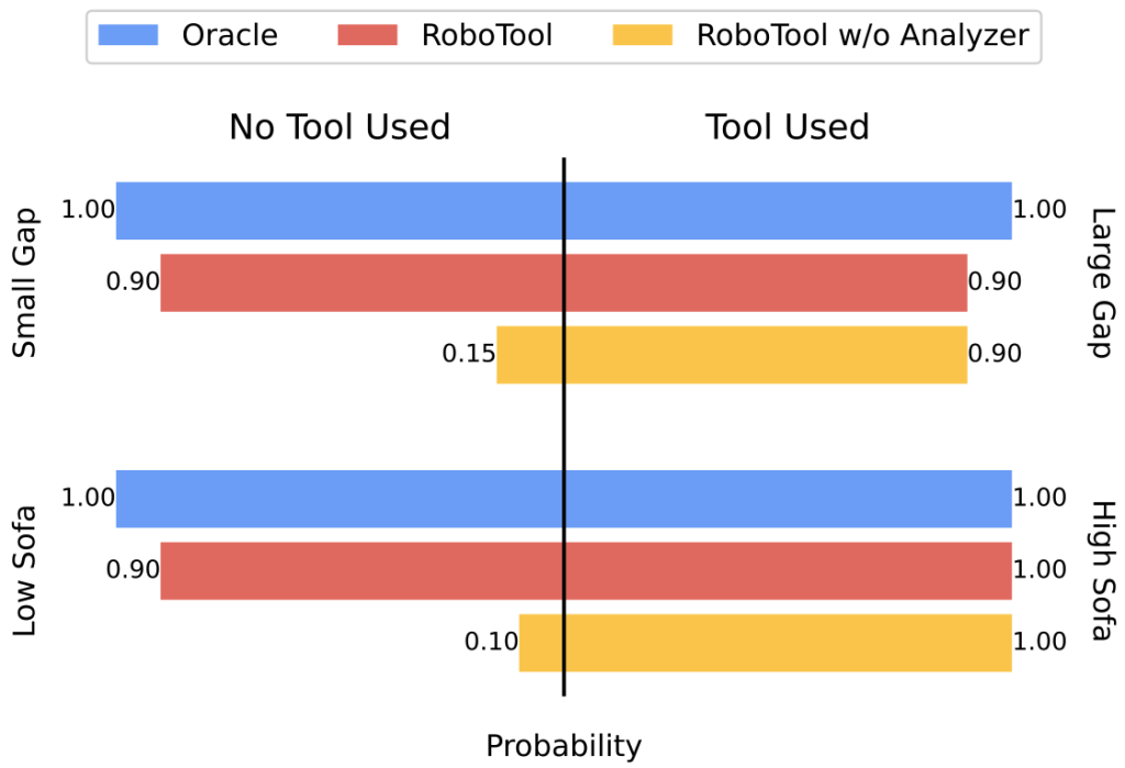
Importantly, we found that most models still struggle with GenAI-Bench prompts, indicating significant room for improvement:
State-of-the-art models such as DALL-E 3, SD-XL, Pika, and Gen2 still fail to handle compositional prompts of GenAI-Bench!
Improving Text-to-Image Generation with VQAScore
Lastly, we demonstrate how VQAScore can improve text-to-image generation in a black-box manner [Liu et al., CVPR 2024] by selecting the highest-VQAScore images from as few as three generated candidates:
VQAScore can improve DALL-E 3 on challenging GenAI-Bench prompts using its black-box API to rank the three generated candidate images. We encourage readers to refer to our paper for the full experimental setup and human evaluation results!
Conclusion
Metrics and benchmarks play a crucial role in the evolution of science. We hope that VQAScore and GenAI-Bench provide new insights into the evaluation of text-to-visual models and offer a robust, reproducible alternative to costly human evaluations.
References:
Lin et al., Evaluating Text-to-Visual Generation with Image-to-Text Generation. ECCV 2024.
Li et al., GenAI-Bench: Evaluating and Improving Compositional Text-to-Visual Generation. CVPR SynData 2024 Workshop, Best Short Paper.
Lin et al., Revisiting the Role of Language Priors in Vision-Language Models. ICML 2024.
Liu et al., Language Models as Black-Box Optimizers for Vision-Language Models. CVPR 2024.
Parashar et al., The Neglected Tails in Vision-Language Models. CVPR 2024.
Hessel et al., A Reference-free Evaluation Metric for Image Captioning. EMNLP 2021.
Heusel et al., GANs Trained by a Two Time-Scale Update Rule Converge to a Local Nash Equilibrium. NeurIPS 2017.
Betker et al., Improving Image Generation with Better Captions (DALL-E 3). OpenAI 2023.
Esser et al., Scaling Rectified Flow Transformers for High-Resolution Image Synthesis. Stability AI 2024.
Zhang et al., The Unreasonable Effectiveness of Deep Features as a Perceptual Metric. CVPR 2018.
Thrush et al., Winoground: Probing Vision and Language Models for Visio-Linguistic Compositionality. CVPR 2022.
Yuksekgonul et al., When and why vision-language models behave like bags-of-words, and what to do about it? ICLR 2023.
Advances in generative models have made it possible for AI-generated text, code, and images to mirror human-generated content in many applications. Watermarking, a technique that embeds information in the output of a model to verify its source, aims to mitigate the misuse of such AI-generated content. Current state-of-the-art watermarking schemes embed watermarks by slightly perturbing probabilities of the LLM’s output tokens, which can be detected via statistical testing during verification.
Unfortunately, our work shows that common design choices in LLM watermarking schemes make the resulting systems surprisingly susceptible to watermark removal or spoofing attacks—leading to fundamental trade-offs in robustness, utility, and usability. To navigate these trade-offs, we rigorously study a set of simple yet effective attacks on common watermarking systems and propose guidelines and defenses for LLM watermarking in practice.
Prompt
Alan Turing was born in …
Unwatermarked Z-Score: 0.16 ↓ PPL: 3.19
Alan Turing was born in1912 and diedin1954.He was anEnglishmathematician,logician, cryptanalyst,and computerscientist. In1938,Turing joinedthe Government Code and Cypher School (GC&CS), where hecontributed to the design of the bombe,a machinethat was usedto decipher the Enigma-enciphered messages…
Watermarked Z-Score: 5.98 ↑ PPL: 4.46
Alan Turing was born in1912 anddiedin 1954, attheage of41. He was the brilliant British scientist andmathematician whois largely credited with beingthefatherofmodern computer science. He is known for his contributions to mathematicalbiologyand chemistry. He was also one ofthepioneers of computerscience…
Alan Turing was born in1950and died in 1994, at the age of 43. He was the brilliant American scientist and mathematician who is largely credited with being the father of modern computer science. He is known for his contributions to mathematical biology and musicology. He was also one of the pioneers of computer science…
Alan Turing was born in1912 and died in 1954. He was a mathematician, logician, cryptologist and theoretical computer scientist. He is famous for his work on code-breaking and artificial intelligence, and his contribution to the Allied victory in World War II. Turing was born in London. He showed an interest in mathematics…
(c) Watermark-removal attack Exploiting public detection API Z-Score: 1.47 ↓ PPL: 4.57
Alan Turing was born in1912 and died in 1954. He was an English mathematician, computer scientist, cryptanalystand philosopher. Turing was a leading mathematicianand cryptanalyst. He was one of the key players in cracking the German Enigma Code during World War II. He also came up with the Turing Machine…
Table 1. Examples generated using LLAMA-2-7B with/without the KGW watermark under various attacks. The watermark will split the vocabulary into green and red lists and give preference for words in the green list. Z-score reflects the detection confidence of the watermark, and perplexity (PPL) measures text quality. (a) In the piggyback spoofing attack, we exploit watermark robustness by generating incorrect content that appears as watermarked (matching the z-score of the watermarked baseline), potentially damaging the reputation of the LLM. Incorrect tokens modified by the attacker are marked in orange and watermarked tokens in blue. (b-c) In watermark-removal attacks, attackers can effectively lower the z-score below the detection threshold while preserving a high sentence quality (low PPL) by exploiting either the (b) use of multiple keys or (c) publicly available watermark detection APIs.
What is LLM Watermarking?
Similar to image watermarks, LLM watermarking embeds invisible secret patterns into the text. Here, we briefly introduce LLMs and LLM watermarks. We use (x) to denote a sequence of tokens, (x_i in mathcal{V}) represents the (i)-th token in the sequence, and (mathcal{V}) is the vocabulary. (M_{text{orig}}) denotes the original model without a watermark, (M_{text{wm}}) is the watermarked model, and (sk in mathcal{S}) is the watermark secret key sampled from (mathcal{S}).
Language Model. State-of-the-art (SOTA) LLMs are auto-regressive models, which predict the next token based on the prior tokens. We define language models more formally below:
Definition 1 (Language Model). A language model (LM) without a watermark is a mapping: $$ M_{text{orig}}: mathcal{V}^* rightarrow mathcal{V}, $$ where the input is a sequence of length (t) tokens (x). (M_{text{orig}}(textbf{x})) first returns the probability distribution for the next token, then (x_{t+1}) is sampled from this distribution.
Figure 1. LLM predicts the next tokens auto-regressively.
Watermarks for LLMs. We focus on SOTA decoding-based robust watermarking schemes including KGW, Unigram, and Exp. In each of these methods, the watermarks are embedded by perturbing the output distribution of the original LLM. The perturbation is determined by secret watermark keys held by the LLM owner. Formally, we define the watermarking scheme:
Definition 2 (Watermarked LLMs). The watermarked LLM takes token sequence (x in mathcal{V}^* ) and secret key (sk in mathcal{S}) as input, and outputs a perturbed probability distribution for the next token. The perturbation is determined by (sk):
$$M_{text{wm}} : mathcal{V}^* times mathcal{S} rightarrow mathcal{V}$$
The watermark detection outputs the statistical testing score for the null hypothesis that the input token sequence is independent of the watermark secret key: $$f_{text{detection}} : mathcal{V}^* times mathcal{S} rightarrow mathbb{R}$$ The output score reflects the confidence of the watermark’s existence in the input.
Figure 2. Watermark is embedded by perturbing the probability distribution of the next token. The perturbation is determined by the secret key (sk).
Common Design Choices of LLM Watermarks
There are a number of common design choices in existing LLM watermarking schemes, including robustness, the use of multiple keys, and public detection APIs that have clear benefits to enhance watermark security and usability. We describe these key design choices briefly below, and then explain how an attacker can easily take advantage of these design choices to launch watermark removal or spoofing attacks.
Robustness. The goal of developing a watermark that is robust to output perturbations is to defend against watermark removal, which may be used to circumvent detection schemes for applications such as phishing or fake news generation. Robust watermark designs have been the topic of many recent works. A more robust watermark can better defend against watermark-removal attacks. However, our work shows that robustness can also enable piggyback spoofing attacks.
Multiple Keys. Many works have explored the possibility of launching watermark stealing attacks to infer the secret pattern of the watermark, which can then boost the performance of spoofing and removal attacks. A natural and effective defense against watermark stealing is using multiple watermark keys during embedding, which can improve the unbiasedness property of the watermark (it is called distortion-free in the Exp watermark). Rotating multiple secret keys is a common practice in cryptography and is also suggested by prior watermarks. More keys being used during embedding indicates better watermark unbiasedness and thus it becomes more difficult for attackers to infer the watermark pattern. However, we show that using multiple keys can also introduce new watermark-removal vulnerabilities.
Public Detection API. It is still an open question whether watermark detection APIs should be made publicly available to users. Although this makes it easier to detect watermarked text, it is commonly acknowledged that it will make the system vulnerable to attacks. We study this statement more precisely by examining the specific risk trade-offs that exist, as well as introducing a novel defense that may make the public detection API more feasible in practice.
Attacks, Defenses, and Guidelines
Although the above design choices are beneficial for enhancing the security and usability of watermarking systems, they also introduce new vulnerabilities. Our work studies a set of simple yet effective attacks on common watermarking systems and propose guidelines and defenses for LLM watermarking in practice.
In particular, we study two types of attacks—watermark-removal attacks and (piggyback or general) spoofing attacks. In the watermark-removal attack, the attacker aims to generate a high-quality response from the LLM without an embedded watermark. For the spoofing attacks, the goal is to generate a harmful or incorrect output that has the victim organization’s watermark embedded.
Piggyback Spoofing Attack Exploiting Robustness
More robust watermarks can better defend against editing attacks, but this seemingly desirable property can also be easily misused by malicious users to launch simple piggyback spoofing attacks. In piggyback spoofing attacks, a small portion of toxic or incorrect content is inserted into the watermarked material, making it seem like it was generated by a specific watermarked LLM. The toxic content will still be detected as watermarked, potentially damaging the reputation of the LLM service provider.
Attack Procedure. (i) The attacker queries the target watermarked LLM to receive a high-entropy watermarked sentence (x_{wm}), (ii) The attacker edits (x_{wm}) and forms a new piece of text (x’) and claims that (x’) is generated by the target LLM. The editing method can be defined by the attacker. Simple strategies could include inserting toxic tokens into the watermarked sentence (x_{wm}), or editing specific tokens to make the output inaccurate. As we show, editing can be done at scale by querying another LLM like GPT4 to generate fluent output.
Results. We show that piggyback spoofing can generate fluent, watermarked, but inaccurate results at scale. Specifically, we edit the watermarked sentence by querying GPT4 using the prompt "Modify less than 3 words in the following sentence and make it inaccurate or have opposite meanings."
Figure 3. Piggyback spoofing on KGW and LLAMA-2-7B. Lower perplexity (PPL) indicates higher sentence quality. Higher z-score reflects higher confidence in watermarking.
Figure 3 shows that we can successfully generate fluent results, with a slightly higher PPL. 94.17% of the piggyback results have a z-score higher than the detection threshold 4. We randomly sample 100 piggyback results and manually check that most of them (92%) are fluent and have inaccurate or opposite content from the original watermarked content. We present a spoofing sentence below. For more results, please check our manuscript.
Watermarked content, z-score: 4.93, PPL: 4.61 Earth has a history of 4.5 billion years and humans have been around for 200,000 years. Yet humans have been using computers for just over 70 years and even then the term was first used in 1945. In the age of technology, we are still just getting started. The first computer, ENIAC (Electronic Numerical Integrator And Calculator), was built at the University of Pennsylvania between 1943 and 1946. The ENIAC took up 1800 sq ft and had 18,000 vacuum tube and mechanical parts. The ENIAC was used for mathematical calculations, ballistics, and code breaking. The ENIAC was 1000 times faster than any other calculator of the time. The first computer to run a program was the Z3, built by Konrad Zuse at his house.
Piggyback attack, z-score: 4.36, PPL: 5.68 Earth has a history of 4.5 billion years and humans have been around for 200,000 years. Yet humans have been using computers for just over 700 years and even then the term was first used in 1445. In the age of technology, we are still just getting started. The first computer, ENIAC (Electronic Numerical Integrator And Calculator), was built at the University of Pennsylvania between 1943 and 1946. The ENIAC took up 1800 sq ft and had 18,000 vacuum tube and mechanical parts. The ENIAC was used for mathematical calculations, ballistics, and code breaking. The ENIAC was 1000 times slower than any other calculator of the time. The first computer to run a program was the Z3, built by Konrad Zuse at his house.
Discussion. Piggyback spoofing attacks are easy to execute in practice. Robust LLM watermarks typically do not consider such attacks during design and deployment, and existing robust watermarks are inherently vulnerable to such attacks. We consider this attack to be challenging to defend against, especially considering the examples presented above, where by only editing a single token, the entire content becomes incorrect. It is hard, if not impossible, to detect whether a particular token is from the attacker by using robust watermark detection algorithms. Recently, researchers proposed publicly detectable watermarks that plant a cryptographic signature into the generated sentence [Fairoze et al. 2024]. They mitigate such piggyback spoofing attacks at the cost of sacrificing robustness. Thus, practitioners should weigh the risks of removal vs. piggyback spoofing attacks for the model at hand.
Guideline #1. Robust watermarks are vulnerable to spoofing attacks and are not suitable as proof of content authenticity alone. To mitigate spoofing while preserving robustness, it may be necessary to combine additional measures such as signature-based fragile watermarks.
Watermark-Removal Attack Exploiting Multiple Keys
SOTA watermarking schemes aim to ensure the watermarked text retains its high quality and the private watermark patterns are not easily distinguished by maintaining an unbiasedness property: $$|mathbb{E}_{sk in mathcal{S}}[M_{text{wm}}(textbf{x}, sk)] – M_text{orig}(textbf{x})| = O(epsilon),$$ i.e., the expected distribution of watermarked output over the watermark key space (sk in S) is close to the output distribution without a watermark, differing by a distance of (epsilon). Exp is rigorously unbiased, and KGW and Unigram slightly shift the watermarked distributions.
We consider multiple keys to be used during watermark embedding to defend against watermark stealing attacks. The insight of our proposed watermark-removal attack is that, given the “unbiased” nature of watermarks, malicious users can estimate the output distribution without any watermark by repeatedly querying the watermarked LLM using the same prompt. As this attack estimates the original, unwatermarked distribution, the quality of the generated content is preserved.
Attack Procedure. (i) An attacker queries a watermarked model with an input (x) multiple times, observing (n) subsequent tokens (x_{t+1}). (ii) The attacker then creates a frequency histogram of these tokens and samples according to the frequency. This sampled token matches the result of sampling on an unwatermarked output distribution with a nontrivial probability. Consequently, the attacker can progressively eliminate watermarks while maintaining a high quality of the synthesized content.
Results. We study the trade-off between resistance against watermark stealing and watermark-removal attacks by evaluating a recent watermark stealing attack [Jovanović et al. 2024], where we query the watermarked LLM to obtain 2.2 million tokens to “steal” the watermark pattern and then launch spoofing attacks using the estimated watermark pattern. In our watermark removal attack, we consider that the attacker has observations with different keys.
Figure 4a. Z-Score and attack success rate (ASR) of watermark stealing on KGW watermark and LLAMA-2-7B model with different watermark keys (n).
Figure 4b. Z-Score and attack success rate (ASR) of watermark-removal on KGW watermark and LLAMA-2-7B model with different watermark keys (n).
Figure 4c. Perplexity (PPL) of watermark-removal on KGW watermark and LLAMA-2-7B model with different watermark keys (n).
As shown in Figure 4a, using multiple keys can effectively defend against watermark stealing attacks. With a single key, the ASR is 91%. We observe that using three keys can effectively reduce the ASR to 13%, and using more than 7 keys, the ASR of the watermark stealing is close to zero. However, using more keys also makes the system vulnerable to our watermark-removal attacks as shown in Figure 4b. When we use more than 7 keys, the detection scores of the content produced by our watermark removal attacks closely resemble those of unwatermarked content and are much lower than the detection thresholds, with ASRs higher than 97%. Figure 4c suggests that using more keys improves the quality of the output content. This is because, with a greater number of keys, there is a higher probability for an attacker to accurately estimate the unwatermarked distribution.
Discussion. Many prior works have suggested using multiple keys to defend against watermark stealing attacks. However, we reveal that a conflict exists between improving resistance to watermark stealing and the feasibility of removing watermarks. Our results show that finding a “sweet spot” in terms of the number of keys to use to mitigate both the watermark stealing and the watermark-removal attacks is not trivial. Given this tradeoff, we suggest that LLM service providers consider “defense-in-depth” techniques such as anomaly detection, query rate limiting, and user identification verification.
Guideline #2. Using a larger number of watermarking keys can defend against watermark stealing attacks, but increases vulnerability to watermark-removal attacks. Limiting users’ query rates can help to mitigate both attacks.
Attacks Exploiting Public Detection APIs
Fially, we show that publicly available detection APIs can enable both spoofing and removal attacks. The insight is that by querying the detection API, the attacker can gain knowledge about whether a specific token is carrying the watermark or not. Thus, the attacker can select the tokens based on the detection result to launch spoofing and removal attacks.
Attack Procedure. (i) An attacker feeds a prompt into the watermarked LLM (removal attack) or into a local LLM (spoofing attack), which generates the response in an auto-regressive manner. For the token (x_i) the attacker will generate a list of possible replacements for (x_i). (ii) The attacker will query the detection using these replacements and sample a token based on their probabilities and detection scores to remove or spoof the watermark while preserving a high output quality. This replacement list can be generated by querying the watermarked LLM, querying a local model, or simply returned by the watermarked LLM (e.g., enabled by OpenAI’s API top_logprobs=5).
Results. We evaluate the detection scores for both the watermark-removal and the spoofing attacks. Furthermore, for the watermark-removal attack, where the attackers care more about the output quality, we report the output PPL.
Figure 5a. Z-Score/P-Value of watermark removal using detection APIs on LLAMA-2-7B and different watermarks.
Figure 5b. The perplexity of watermark removal using detection APIs on LLAMA-2-7B and different watermarks.
Figure 5c. Z-Score/P-Value of watermark spoofing using detection APIs on LLAMA-2-7B and different watermarks.
As shown in Figure 5a and Figure 5b, watermark-removal attacks exploiting the detection API significantly reduce detection confidence while maintaining high output quality. For instance, for the KGW watermark on LLAMA-2-7B model, we achieve a median z-score of 1.43, which is much lower than the threshold 4. The PPL is also close to the watermarked outputs (6.17 vs. 6.28). We observe that the Exp watermark has higher PPL than the other two watermarks. A possible reason is that Exp watermark is deterministic, while other watermarks enable random sampling during inference. Our attack also employs sampling based on the token probabilities and detection scores, thus we can improve the output quality for the Exp watermark. The spoofing attacks also significantly boost the detection confidence even though the content is not from the watermarked LLM, as depicted in Figure 5c.
Defending Detection with Differential Privacy. In light of the issues above, we propose an effective defense using ideas from differential privacy (DP) to counteract the detection API based spoofing attacks. DP adds random noise to function results evaluated on private datasets such that the results from neighboring datasets are indistinguishable. Similarly, we consider adding Gaussian noise to the distance score in the watermark detection, making the detection ((epsilon, delta))-DP, and ensuring that attackers cannot tell the difference between two queries by replacing a single token in the content, thus increasing the hardness of launching the attacks.
Figure 6a. Spoofing attack success rate (ASR) and detection accuracy (ACC) without and with DP watermark detection under different noise parameters.
Figure 6b. Z-scores of original text without attack, spoofing attack without DP defense, and spoofing attacks with DP defense. We use the best (sigma=4) from Figure 6a.
As shown in Figure 6, with a noise scale of (sigma=4), the DP detection’s accuracy drops from the original 98.2% to 97.2% on KGW and LLAMA-2-7B, while the spoofing ASR becomes 0%. The results are consistent for other watermarks and models.
Discussion. The detection API, available to the public, aids users in differentiating between AI and human-created materials. However, it can be exploited by attackers to gradually remove watermarks or launch spoofing attacks. We propose a defense utilizing the ideas in differential privacy. Even though the attacker can still obtain useful information by increasing the detection sensitivity, our defense significantly increases the difficulty of spoofing attacks. However, this method is less effective against watermark-removal attacks that exploit the detection API because attackers’ actions will be close to random sampling, which, even though with lower success rates, remains an effective way of removing watermarks. Therefore, we leave developing a more powerful defense mechanism against watermark-removal attacks exploiting detection API as future work. We recommend companies providing detection services should detect and curb malicious behavior by limiting query rates from potential attackers, and also verify the identity of the users to protect against Sybil attacks.
Guideline #3. Public detection APIs can enable both spoofing and removal attacks. To defend against these attacks, we propose a DP-inspired defense, which combined with techniques such as anomaly detection, query rate limiting, and user identification verification can help to make public detection more feasible in practice.
Conclusion
Although LLM watermarking is a promising tool for auditing the usage of LLM-generated text, fundamental trade-offs exist in the robustness, usability, and utility of existing approaches. In particular, our work shows that it is easy to take advantage of common design choices in LLM watermarks to launch attacks that can easily remove the watermark or generate falsely watermarked text. Our study finds that these vulnerabilities are common to existing LLM watermarks and provides caution for the field in deploying current solutions in practice without carefully considering the impact and trade-offs of watermarking design choices. To establish more reliable future LLM watermarking systems, we also suggest guidelines for designing and deploying LLM watermarks along with possible defenses motivated by the theoretical and empirical analyses of our attacks. For more results and discussions, please see our manuscript.
A central question in the discussion of large language models (LLMs) concerns the extent to which they memorize their training data versus how they generalize to new tasks and settings. Most practitioners seem to (at least informally) believe that LLMs do some degree of both: they clearly memorize parts of the training data—for example, they are often able to reproduce large portions of training data verbatim [Carlini et al., 2023]—but they also seem to learn from this data, allowing them to generalize to new settings. The precise extent to which they do one or the other has massive implications for the practical and legal aspects of such models [Cooper et al., 2023]. Do LLMs truly produce new content, or do they only remix their training data? Should the act of training on copyrighted data be deemed an unfair use of data, or should fair use be judged by some notion of model memorization? When dealing with humans, we distinguish plagiarizing content from learning from it, but how should this extend to LLMs? The answer inherently relates to the definition of memorization for LLMs and the extent to which they memorize their training data.
However, even defining memorization for LLMs is challenging, and many existing definitions leave much to be desired. In our recent paper (project page), we propose a new definition of memorization based on a compression argument. Our definition posits that
a phrase present in the training data is memorized if we can make the model reproduce the phrase using a prompt (much) shorter than the phrase itself.
Operationalizing this definition requires finding the shortest adversarial input prompt that is specifically optimized to produce a target output. We call this ratio of input-to-output tokens the Adversarial Compression Ratio (ACR). In other words, memorization is inherently tied to whether a certain output can be represented in a compressed form beyond what language models can do with typical text. We argue that such a definition provides an intuitive notion of memorization. If a certain phrase exists within the LLM training data (e.g., is not itself generated text) and it can be reproduced with fewer input tokens than output tokens, then the phrase must be stored somehow within the weights of the LLM. Although it may be more natural to consider compression in terms of the LLM-based notions of input/output perplexity, we argue that a simple compression ratio based on input/output token counts provides a more intuitive explanation to non-technical audiences and has the potential to serve as a legal basis for important questions about memorization and permissible data use. In addition to its intuitive nature, our definition has several other desirable qualities. We show that it appropriately ascribes many famous quotes as being memorized by existing LLMs (i.e., they have high ACR values). On the other hand, we find that text not in the training data of an LLM, such as samples posted on the internet after the training period, are not compressible, that is their ACR is low.
We examine several unlearning methods using ACR to show that they do not substantially affect the memorization of the model. That is, even after explicit finetuning, models asked to “forget” certain pieces of content are still able to reproduce them with a high ACR—in fact, not much smaller than with the original model. Our approach provides a simple and practical perspective on what memorization can mean, providing a useful tool for functional and legal analysis of LLMs.
Why We Need A New Definition
With LLMs ingesting more and more data, questions about their memorization are attracting attention [e.g., Carlini et al., 2019, 2023;Nasr et al., 2023;Zhang et al., 2023]. There remains a pressing need to accurately define memorization in a way that serves as a practical tool to ascertain the fair use of public data from a legal standpoint. To ground the problem, consider the court’s role in determining whether an LLM is breaching copyright. What constitutes a breach of copyright remains contentious, and prior work defines this on a spectrum from ‘training on a data point itself constitutes violation’ to ‘copyright violation only occurs if a model verbatim regurgitates training data.’ To formalize our argument for a new notion of memorization, we start with three definitions from prior work to highlight some of the gaps in the current thinking about memorization.
Discoverable memorization [Carlini et al., 2023], which says a string is memorized if the first few words elicit the rest of the quote exactly, has three particular problems. It is very permissive, easy to evade, and requires validation data to set parameters. Another notion is Extractable Memorization [Nasr et al., 2023], which says that if there exists a prompt that elicits the string in response. This falls too far on the other side of the issue by being very restrictive—what if the prompt includes the entire string in question, or worse, the instructions to repeat it? LLMs that are good at repeating will follow that instruction and output any string they are asked to. The risk is that it is possible to label any element of the training set as memorized, rendering this definition unfit in practice. Another definition is Counterfactual Memorization [Zhang et al., 2023], which aims to separate memorization from generalization and is tested through retraining many LLMs. Given the cost of training LLMs, such a definition is impractical for legal use.
In addition to these definitions from prior work on LLM memorization, several other seemingly viable approaches to memorization exist. Ultimately, we argue all of these frameworks—the definitions in existing work and the approaches described below—are each missing key elements of a good definition for assessing fair use of data.
Membership is not memorization. Perhaps if a copyrighted piece of data is in the training set at all, we might consider it a problem. However, there is a subtle but crucial difference between training set membership and memorization. In particular, the ongoing lawsuits in the field [e.g., as covered by Metz and Robertson, 2024] leave open the possibility that reproducing another’s creative work is problematic, but training on samples from that data may not be. This is common practice in the arts—consider that a copycat comedian telling someone else’s jokes is stealing, but an up-and-comer learning from tapes of the greats is doing nothing wrong. So while membership inference attacks (MIAs) [e.g. Shokri et al., 2017] may look like tests for memorization and they are even intimately related to auditing machine unlearning [Carlini et al., 2021, Pawelczyk et al., 2023, Choi et al., 2024], they have three issues as tests for memorization. Specifically, they are very restrictive, they are hard to arbitrate, and evaluation techniques are brittle.
Adversarial Compression Ratio
Our definition of memorization is based on answering the following question: Given a piece of text, how short is the minimal prompt that elicits that text exactly? In this section, we formally define and introduce our MiniPrompt algorithm that we use to answer our central question.
To begin, let a target natural text string (s) have a token sequence representation (xin mathcal V^*), which is a list of integer-valued indices that index a given vocabulary (mathcal V). We use (|cdot|) to count the length of a token sequence. A tokenizer (T:smapsto x) maps from strings to token sequences. Let (M) be an LLM that takes a list of tokens as input and outputs the next token probabilities. Consider that (M) can perform generation by repeatedly predicting the next token from all the previous tokens with the argmax of its output appended to the sequence at each step (this process is called greedy decoding). With a slight abuse of notation, we will also call the greedy decoding result the output of (M). Let (y) be the token sequence generated by (M), which we call a completion or response: (y = M(x)), which in natural language says that the model generates (y) when prompted with (x) or that (x) elicits (y) as a response from (M). So our compression ratio ACR is defined for a target sequence (y) as ACR((M, y) = frac{|y|}{|x^*|}), where (x^* = text{argmin}_{x} |x|) s.t. (M(x) = y).
Definition [(tau)-Compressible Memorization] Given a generative model (M), a sample (y) from the training data is (tau)-memorized if the ACR((M, y) > tau(y)).
The threshold (tau(y)) is a configurable parameter of this definition. We might choose to compare the ACR to the compression ratio of the text when run through a general-purpose compression program (explicitly assumed not to have memorized any such text) such as GZIP [Gailly and Adler, 1992] or SMAZ [Sanfilippo, 2006]. This amounts to setting (tau(y)) equal to the SMAZ compression ratio of (y), for example. Alternatively, one might even use the compression ratio of the arithmetic encoding under another LLM as a comparison point, for example, if it was known with certainty that the LLM was never trained on the target output and hence could not have memorized it [Delétang et al., 2023]. In reality, copyright attribution cases are always subjective, and the goal of this work is not to argue for the right threshold function but rather to advocate for the adversarial compression framework for arbitrating fair data use. Thus, we use (tau = 1), which we believe has substantial practical value. 1
Our definition and the compression ratio lead to two natural ways to aggregate over a set of examples. First, we can average the ratio over all samples/test strings and report the average compression ratio (this is (tau)-independent). Second, we can label samples with a ratio greater than one as memorized and discuss the portion memorized over some set of test cases (for our choice of (tau =1 )).
Empirical Findings
Model Size vs. Memorization: Since prior work has proposed alternative definitions of memorization that show that bigger models memorize more [Carlini et al., 2023], we ask whether our definition leads to the same finding. We find the same trends under our definition, meaning our view of memorization is consistent with existing scientific findings.
Unlearning for Privacy: We further experiment with models finetuned on synthetic data, which show that completion-based tests (i.e., the model’s ability to generate a specific output) often fail to fully reflect the model’s memorization. However, the ACR captures the persistence of memorization even after moderate attempts at unlearning.
Four Categorties of Data for Validation: We also validate the ACR as a metric using four different types of data: random sequences, famous quotes, Wikipedia sentences, and recent Associated Press (AP) articles. The goal is to ensure that the ACR aligns with intuitive expectations of memorization. Our results show that random sequences and recent AP articles, which the models were not trained on, are not compressible (i.e., not memorized). Famous quotes, which are repeated in the training data, show high compression ratios, indicating memorization. Wikipedia sentences fall between the two extremes, as some of them are memorized. These results validate that ACR meaningfully identifies memorization in data that is more common or repeated in the training set, while appropriately labelling unseen data as not-memorized.
When proposing new definitions, we are tasked with justifying why a new one is needed as well as showing its ability to capture a phenomenon of interest. This stands in contrast to developing detection/classification tools whose accuracy can easily be measured using labeled data. It is difficult by nature to define memorization as there is no set of ground truth labels that indicate which samples are memorized. Consequently, the criteria for a memorization definition should rely on how useful it is. Our definition is a promising direction for future regulation on LLM fair use of data as well as helping model owners confidently release models trained on sensitive data without releasing that data. Deploying our framework in practice may require careful thought about how to set the compression threshold but as it relates to the legal setting this is not a limitation as law suits always have some subjectivity [Downing, 2024]. Furthermore, as evidence in a court, this metric would not provide a binary test on which a suit could be decided, rather it would be a piece of a batch of evidence, in which some is more probative than others. Our hope is to provide regulators, model owners, and the courts a mechanism to measure the extent to which a model contains a particular string within its weights and make discussion about data usage more grounded and quantitative.
References
Nicholas Carlini, Chang Liu, Úlfar Erlingsson, Jernej Kos, and Dawn Song. The secret sharer: Evaluating and testing unintended memorization in neural networks. In 28thUSENIX security symposium (USENIX security 19), pages 267–284, 2019.
Nicholas Carlini, Steve Chien, Milad Nasr, Shuang Song, Andreas Terzis, and Florian Tramer. Membership inference attacks from first principles. arXiv preprint arXiv:2112.03570, 2021.
Nicholas Carlini, Daphne Ippolito, Matthew Jagielski, Katherine Lee, Florian Tramer, and Chiyuan Zhang. Quantifying memorization across neural language models, 2023.
Dami Choi, Yonadav Shavit, and David K Duvenaud. Tools for verifying neural models’ training data. Advances in Neural Information Processing Systems, 36, 2024.
A Feder Cooper, Katherine Lee, James Grimmelmann, Daphne Ippolito, Christo- pher Callison-Burch, Christopher A Choquette-Choo, Niloofar Mireshghallah, Miles Brundage, David Mimno, Madiha Zahrah Choksi, et al. Report of the 1st workshop on generative ai and law. arXiv preprint arXiv:2311.06477, 2023.
Grégoire Delétang, Anian Ruoss, Paul-Ambroise Duquenne, Elliot Catt, Tim Genewein, Christopher Mattern, Jordi Grau-Moya, Li Kevin Wenliang, Matthew Aitchison, Laurent Orseau, et al. Language modeling is compression. arXiv preprint arXiv:2309.10668, 2023.
Kate Downing. Copyright fundamentals for AI researchers. In Proceedings of the Twelfth International Conference on Learning Representations (ICLR), 2024. URL https://iclr.cc/media/iclr-2024/Slides/21804.pdf.
Jean-Loup Gailly and Mark Adler. gzip. https://www.gnu.org/software/gzip/, 1992. Accessed: 2024-05-21.
Cade Metz and Katie Robertson. Openai seeks to dismiss parts of the new york times’s lawsuit. The New York Times, 2024. URL https://www.nytimes.com/2024/02/27/ technology/openai-new-york-times-lawsuit.html#: ̃:text=In%20its%20suit% 2C%20The%20Times,someone%20to%20hack%20their%20chatbot.
Milad Nasr, Nicholas Carlini, Jonathan Hayase, Matthew Jagielski, A Feder Cooper, Daphne Ippolito, Christopher A Choquette-Choo, Eric Wallace, Florian Tram`er, and Katherine Lee. Scalable extraction of training data from (production) language models. arXiv preprint arXiv:2311.17035, 2023.
Martin Pawelczyk, Seth Neel, and Himabindu Lakkaraju. In-context unlearning: Language models as few shot unlearners. arXiv preprint arXiv:2310.07579, 2023.
Reza Shokri, Marco Stronati, Congzheng Song, and Vitaly Shmatikov. Membership inference attacks against machine learning models. In 2017 IEEE symposium on security and privacy (SP), pages 3–18. IEEE, 2017.
Chiyuan Zhang, Daphne Ippolito, Katherine Lee, Matthew Jagielski, Florian Tramèr, and Nicholas Carlini. Counterfactual memorization in neural language models. Advances in Neural Information Processing Systems, 36:39321–39362, 2023.
Footnotes
1 There exist prompts like “count from (1) to (1000),” for which a chat model (M) is able to generate (1, 2, ldots, 1000),” which results in a very high ACR. However, for copyright purposes, we argue that this category of algorithmic prompts is in the gray area where determining memorization is difficult and beyond the scope of this paper, given our primary application to creative works.
Causal inference is the process of determining whether and how a cause leads to an effect, typically using statistical methods to distinguish correlation from causation. Learning causal relationships from data is an important task across a wide variety of domains ranging from healthcare and drug development, to online advertising and e-commerce. As a result, there has been much work in the literature on economics, statistics, computer science, and public policy on designing algorithms and methodologies for causal inference.
While most of the focus has been on questions which are statistical in nature, one must also take game-theoretic incentives into consideration when doing causal inference about strategic individuals who have a preference over the treatment they receive. For example, it may be hard to infer causal relationships in randomized control trials when there is non-compliance by participants in the study (i.e. when participants do not adhere to the treatment they are assigned). More generally, causal learning may be difficult whenever individuals are free to self-select their own treatments and there is sufficient heterogeneity between individuals with different preferences. Even when compliance can be enforced, individuals may strategize by modifying the attributes they present to the causal inference process in order to be assigned a more desirable treatment.
This annotated reading list is intended to serve as a brief summary of work on causal inference in the presence of strategic agents. While this list is not comprehensive, we hope that it will be a useful starting point for members of the machine learning community to learn more about this exciting research area at the intersection of causal inference and game theory.
The reading list is organized as follows: (1, 3) study non-compliance in randomized trials, (2-4) focus on instrumental variable methods, (4-6) consider incentive misalignment between the individual running the causal inference procedure and the subjects of the procedure, (7,8) study cross-unit interference, and (9,10) are about synthetic control methods.
[Robins 1998]: This paper provides an overview of methods to correct for non-compliance in randomized trials (i.e., non-adherence by trial participants to the treatment assignment protocol).
[Angrist et al. 1996]: This seminal paper outlines the concept of instrumental variables (IVs) and describes how they can be used to estimate causal effects. An IV is a variable that affects the treatment variable but is unrelated to the outcome variable except through its effect on the treatment. IV methods leverage the fact that variation in IVs is independent of any confounding in order to estimate the causal effect of the treatment.
[Ngo et al. 2021]: Unlike prior work on non-compliance in clinical trials, this work leverages tools from information design to reveal information about the effectiveness of the treatments in such a way that participants become incentivized to comply with the treatment recommendations over time.
[Harris et al. 2022]: This paper studies the problem of making decisions about a population of strategic agents. The authors make the novel observation that the assessment rule deployed by the principal is a valid instrument, which allows them to apply standard methods for instrumental variable regression to learn causal relationships in the presence of strategic behavior.
[Miller et al. 2020]: This paper considers the problem of strategic classification, where a principal (i.e. decision maker) makes decisions about a population of strategic agents. Given knowledge of the principal’s deployed assessment rule, the agents may strategically modify their observable features in order to receive a more desirable assessment (e.g., a better interest rate on a loan). The authors are the first to show that designing good incentives for agent improvement (i.e. encouraging strategizing in a way which actually benefits the agent) is at least as hard as orienting edges in the corresponding causal graph.
[Wang et al. 2023]: Incentive misalignment between patients and providers may occur when average treated outcomes are used as quality metrics. Such misalignment is generally undesirable in healthcare domains, as it may lead to decreased patient welfare. To mitigate this issue, this work proposes an alternative quality metric, the total treatment effect, which accounts for counterfactual untreated outcomes. The authors show that rewarding the total treatment effect maximizes total patient welfare.
[Wager and Xu 2021]: Motivated by applications such as ride-sharing and tuition subsidies, this work studies settings in which interventions on one unit (e.g. a person or product) may have effects on others (i.e., cross-unit interference). The authors focus on the problem of setting supply-side payments in a centralized marketplace. They use a mean-field modeling-based approach to model the cross-unit interference, and design a class of experimentation schemes which allow them to optimize payments without disturbing the market equilibrium.
[Li et al. 2023]: Like [Wager and Xu 2021], this paper studies the effects of cross-unit interference, although the interference considered here comes from congestion in a service system. As a result, the interference considered here is dynamic, in contrast to the static interference considered in the previous entry.
[Abadie and Gardeazabal 2003]: This is the first paper on synthetic control methods (SCMs), a popular technique for estimating counterfactuals from longitudinal data. In the SCM setup, there is a pre-intervention time period during which all units are under control, followed by a post-intervention time period when all units undergo exactly one intervention (either the treatment or control). Given a test unit (who was given the treatment) and a set of donor units (who remained under control), SCMs use the pre-treatment data to learn a relationship (usually linear or convex) between the test and donor units. This relationship is then extrapolated to the post-intervention time period in order to estimate the counterfactual trajectory for the test unit under control.
[Ngo et al. 2023]: A common assumption in the literature on SCMs is that of “overlap”: the outcomes for the test unit can be written as a combination (e.g., linear or convex) of the donor units. This work sheds light on this often overlooked assumption and shows that (i) when units select their own treatments and (ii) there is sufficient heterogeneity between units who prefer different treatments, then overlap does not hold. Like [Ngo et al. 2021], the authors use tools from information design and multi-armed bandits to incentivize units to explore different treatments in a way which ensures that the overlap condition will gradually become satisfied over time.
Recently, our CMU-MATH team proudly clinched 2nd place in the Artificial Intelligence Mathematical Olympiad (AIMO) out of 1,161 participating teams, earning a prize of $65,536! This prestigious competition aims to revolutionize AI in mathematical problem-solving, with the ultimate goal of building a publicly-shared AI model capable of winning a gold medal in the International Mathematical Olympiad (IMO). Dive into our blog to discover the winning formula that set us apart in this significant contest.
Background: The AIMO competition
The Artificial Intelligence Mathematical Olympiad (AIMO) Prize, initiated by XTX Markets, is a pioneering competition designed to revolutionize AI’s role in mathematical problem-solving. It pushes the boundaries of AI by solving complex mathematical problems akin to those in the International Mathematical Olympiad (IMO). The advisory committee of AIMO includes Timothy Gowers and Terence Tao, both winners of the Fields Medal. Attracting attention from world-class mathematicians as well as machine learning researchers, the AIMO sets a new benchmark for excellence in the field.
AIMO has introduced a series of progress prizes. The first of these was a Kaggle competition, with the 50 test problems hidden from competitors. The problems are comparable in difficulty to the AMC12 and AIME exams for the USA IMO team pre-selection. The private leaderboard determined the final rankings, which then determined the distribution of $253,952 in the one-million dollar prize pool among the top five teams. Each submitted solution was allocated either a P100 GPU or 2xT4 GPUs, with up to 9 hours to solve the 50 problems.
Just to give an idea about how the problems look like, AIMO provided a 10-problem training set open to the public. Here are two example problems in the set:
Let (k, l > 0) be parameters. The parabola (y = kx^2 – 2kx + l) intersects the line (y = 4) at two points (A) and (B). These points are distance 6 apart. What is the sum of the squares of the distances from (A) and (B) to the origin?
Each of the three-digits numbers (111) to (999) is coloured blue or yellow in such a way that the sum of any two (not necessarily different) yellow numbers is equal to a blue number. What is the maximum possible number of yellow numbers there can be?
The first problem is about analytic geometry. It requires the model to understand geometric objects based on textual descriptions and perform symbolic computations using the distance formula and Vieta’s formulas. The second problem falls under extremal combinatorics, a topic beyond the scope of high school math. It’s notoriously challenging because there’s no general formula to apply; solving it requires creative thinking to exploit the problem’s structure. It’s non-trivial to master all these required capabilities even for humans, let alone language models.
In general, the problems in AIMO were significantly more challenging than those in GSM8K, a standard mathematical reasoning benchmark for LLMs, and about as difficult as the hardest problems in the challenging MATH dataset. The limited computational resources—P100 and T4 GPUs, both over five years old and much slower than more advanced hardware—posed an additional challenge. Thus, it was crucial to employ appropriate models and inference strategies to maximize accuracy within the constraints of limited memory and FLOPs.
Our winning formula
Unlike most teams that relied on a single model for the competition, we utilized a dual-model approach. Our final solutions were derived through a weighted majority voting system, which consists of generating multiple solutions with a policy model, assigning a weight to each solution using a reward model, and then choosing the answer with the highest total weight. Specifically, we paired a policy model—designed to generate problem solutions in the form of computer code—with a reward model—which scored the outputs of the policy model. Our final solutions were derived through a weighted majority voting system, where the answers were generated by the policy model and the weights were determined by the scores from the reward model. This strategy stemmed from our study on compute-optimal inference, demonstrating that weighted majority voting with a reward model consistently outperforms naive majority voting given the same inference budget.
Both models in our submission were fine-tuned from the DeepSeek-Math-7B-RL checkpoint. Below, we detail the fine-tuning process and inference strategies for each model.
Policy model: Program-aided problem solver based on self-refinement
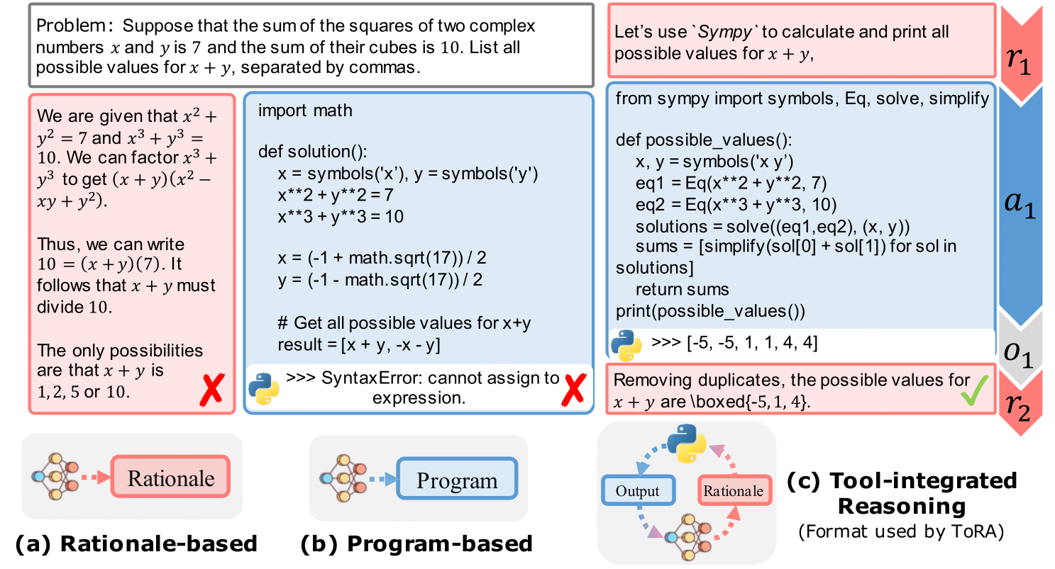
The policy model served as the primary problem solver in our approach. We noted that LLMs can perform mathematical reasoning using both text and programs. Natural language excels in abstract reasoning but falls short in precise computation, symbolic manipulation, and algorithmic processing. Programs, on the other hand, are adept at rigorous operations and can leverage specialized tools like equation solvers for complex calculations. To harness the benefits of both methods, we implemented the Program-Aided Language Models (PAL) or more precisely Tool-Augmented Reasoning (ToRA) approach, originally proposed by CMU & Microsoft. This approach combines natural language reasoning with program-based problem-solving. The model first generates rationales in text form, followed by a computer program which executes to derive a numerical answer
Figure 1: The tool-integrated reasoning format (from ToRA paper)
To train the model, we needed a suitable problem set (the given “training set” of this competition is too small for fine-tuning) with “ground truth” solutions in ToRA format for supervised fine-tuning. Given the problem difficulty (comparable to AMC12 and AIME exams) and the special format (integer answers only), we used a combination of AMC, AIME, and Odyssey-Math as our problem set, removing multiple-choice options and filtering out problems with non-integer answers. This resulted in a dataset of 2,600 problems. We prompted GPT-4o (and DeepSeek-Coder-V2) with few-shot examples to generate 64 solutions for each problem, retaining those that led to correct answers. Our final dataset contained 41,160 problem-solution pairs. We performed supervised fine-tuning on the open-sourced DeepSeek-Math-7B-RL model for 3 epochs with a learning rate of 2e-5.
During inference, we employed the self-refinement technique (which is another widely adopted technique proposed by CMU!), providing feedback to the policy model on the execution results of the generated program (e.g., invalid output, execution failure) and allowing the model to refine the solution accordingly.
Below we present our ablation study on the techniques we employed for the policy model. We used the accuracy on a selected subset of the MATH test set as the evaluation metric. It’s easy to see the combination of techniques that lead to large performance gains compared with naive baselines.
Model
Output format
Inference strategy
Accuracy
DeepSeek RL 7b
Text-only
Greedy decoding
54.02%
DeepSeek RL 7b
ToRA
Greedy decoding
58.05%
DeepSeek RL 7b
ToRA
Greedy + Self-refine
60.73%
DeepSeek RL 7b
ToRA
Maj@16 + Self-refine
70.46%
DeepSeek RL 7b
ToRA
Maj@64 + Self-refine
72.48%
Our finetuned model
ToRA
Maj@16 + Self-refine
74.50%
Our finetuned model
ToRA
Maj@64 + Self-refine
76.51%
Table: Ablation study of our techniques on a selected MATH subset (in which the problems are similar to AIMO problems). Maj@(n) denotes majority voting over (n) sampled solutions.
Notably, the first-place team also used ToRA with self-refinement. However, they curated a much larger problem set of 60,000 problems and used GPT-4 to generate solutions in the ToRA format. Their dataset was more than 20x larger than ours. The cost to generate solutions was far beyond our budget as an academic team (over $100,000 based on our estimation). Our problem set was based purely on publicly available data, and we spent only ~$1,000 for solution generation.
Reward model: Solution scorer using label-balance training
While the policy model was a creative problem solver, it could sometimes hallucinate and produce incorrect solutions. On the publicly available 10-problem training set, our policy model only correctly solved two problems using standard majority voting with 32 sampled solutions. Interestingly, for another 2 problems, the model generated correct solutions that failed to be selected due to wrong answers dominating in majority voting.
This observation highlighted the potential of the reward model. The reward model was a solution scorer that took the policy model’s output and generated a score between 0 and 1. Ideally, it assigned high scores to correct solutions and low scores to incorrect ones, aiding in the selection of correct answers during weighted majority voting.
The reward model was fine-tuned from a DeepSeek-Math-7B-RL model on a labeled dataset containing both correct and incorrect problem-solution pairs. We utilized the same problem set as for the policy model training and expanded it by incorporating problems from the MATH dataset with integer answers. Simple as it may sound, generating high-quality data and training a strong reward model was non-trivial. We considered the following two essential factors for the reward model training set:
Label balance: The dataset should contain both correct (positive examples) and incorrect solutions (negative examples) for each problem, with a balanced number of correct and incorrect solutions.
Diversity: The dataset should include diverse solutions for each problem, encompassing different correct approaches and various failure modes.
Sampling solutions from a single model cannot meet those factors. For example, while our fine-tuned policy model achieved very high accuracy on the problem set, it was unable to generate any incorrect solutions and lacked diversity amongst correct solutions. Conversely, sampling from a weaker model, such as DeepSeek-Math-7B-Base, rarely yielded correct solutions. To create a diverse set of models with varying capabilities, we employed two novel strategies:
Interpolate between strong and weak models. For MATH problems, we interpolated the model parameters of a strong model (DeepSeek-Math-7B-RL) and a weak model (DeepSeek-Math-7B-Base) to get models with different level of capabilities. Denote by (mathbf{theta}_{mathrm{strong}}) and (mathbf{theta}_{mathrm{weak}}) the model parameters of the strong and weak model. We considered interpolated models with parameters (mathbf{theta}_{alpha}=alphamathbf{theta}_{mathrm{strong}}+(1-alpha)mathbf{theta}_{mathrm{weak}}) and set (alphain{0.3, 0.4, cdots, 1.0}), obtaining 8 models. Those models exhibited different problem solving accuracies on MATH. We sampled two solutions from each model for each problem, yielding diverse outputs with balanced correct and incorrect solutions. This technique was motivated by the research on model parameter merging (e.g., model soups) and represented an interesting application of this idea, i.e., generating models with different levels of capabilities.
Leverage intermediate checkpoints. For the AMC, AIME, and Odyssey, recall that our policy model had been fine-tuned on those problems for 3 epochs. The final model and its intermediate checkpoints naturally provided us with multiple models exhibiting different levels of accuracy on these problems. We leveraged these intermediate checkpoints, sampling 12 solutions from each model trained for 0, 1, 2, and 3 epochs.
These strategies allowed us to obtain a diverse set of models almost for free, sampling varied correct and incorrect solutions. We further filtered the generated data by removing wrong solutions with non-integer answers since it was trivial to determine that those answers are incorrect during inference. In addition, for each problem, we maintained equal numbers of correct and incorrect solutions to ensure label balance and avoid a biased reward model. The final dataset contains 7000 unique problems and 37880 labeled problem-solution pairs. We finetuned DeepSeek-Math-7B-RL model for 2 epochs with learning rate 2e-5 on the curated dataset.
Figure 2: Weighted majority voting system based on the policy and reward models.
We validated the effectiveness of our reward model on the public training set. Notably, by pairing the policy model with the reward model and applying weighted majority voting, our method correctly solved 4 out of the 10 problems – while a single policy model could only solve 2 using standard majority voting.
Concluding remarks: Towards machine-based mathematical reasoning
With the models and techniques described above, our CMU-MATH team solved 22 out of 50 problems in the private test set, snagging the second place and establishing the best performance of an academic team. This outcome marks a significant step towards the goal of machine-based mathematical reasoning.
However, we also note that the accuracy achieved by our models still trails behind that of proficient human competitors who can easily solve over 95% of AIMO problems, indicating substantial room for improvement. There are a wide range of directions to be explored:
Advanced inference-time algorithms for mathematical reasoning. Our dual-model approach is a robust technique to enhance model reasoning at inference time. Recent research from our team suggests that more advanced inference-time algorithms, e.g., tree search methods, could even surpass weighted majority voting. Although computational constraints limited our ability to deploy this technique in the AIMO competition, future explorations on optimizing these inference-time algorithms can potentially lead to better mathematical reasoning approaches.
Integration of Automated Theorem Proving. Integrating automated theorem proving (ATP) tools, such as Lean, represents another promising frontier. ATP tools can provide rigorous logical frameworks and support for deeper mathematical analyses, potentially elevating the precision and reliability of problem-solving strategies employed by LLMs. The synergy between LLMs and ATP could lead to breakthroughs in complex problem-solving scenarios, where deep logical reasoning is essential.
Leveraging Larger, More Diverse Datasets. The competition reinforced a crucial lesson about the pivotal role of data in machine learning. Rich, diverse datasets, especially those comprising challenging mathematical problems, are vital for training more capable models. We advocate for the creation and release of larger datasets focused on mathematical reasoning, which would not only benefit our research but also the broader AI and mathematics communities.
Finally, we would like to thank Kaggle and XTX Markets for organizing this wonderful competition. We have open-sourced our code and datasets used in our solution to ensure reproducibility and facilitate future research. We invite the community to explore, utilize, and build upon our work, which is available in our GitHub repository. For further details about our results, please feel free to reach out to us!
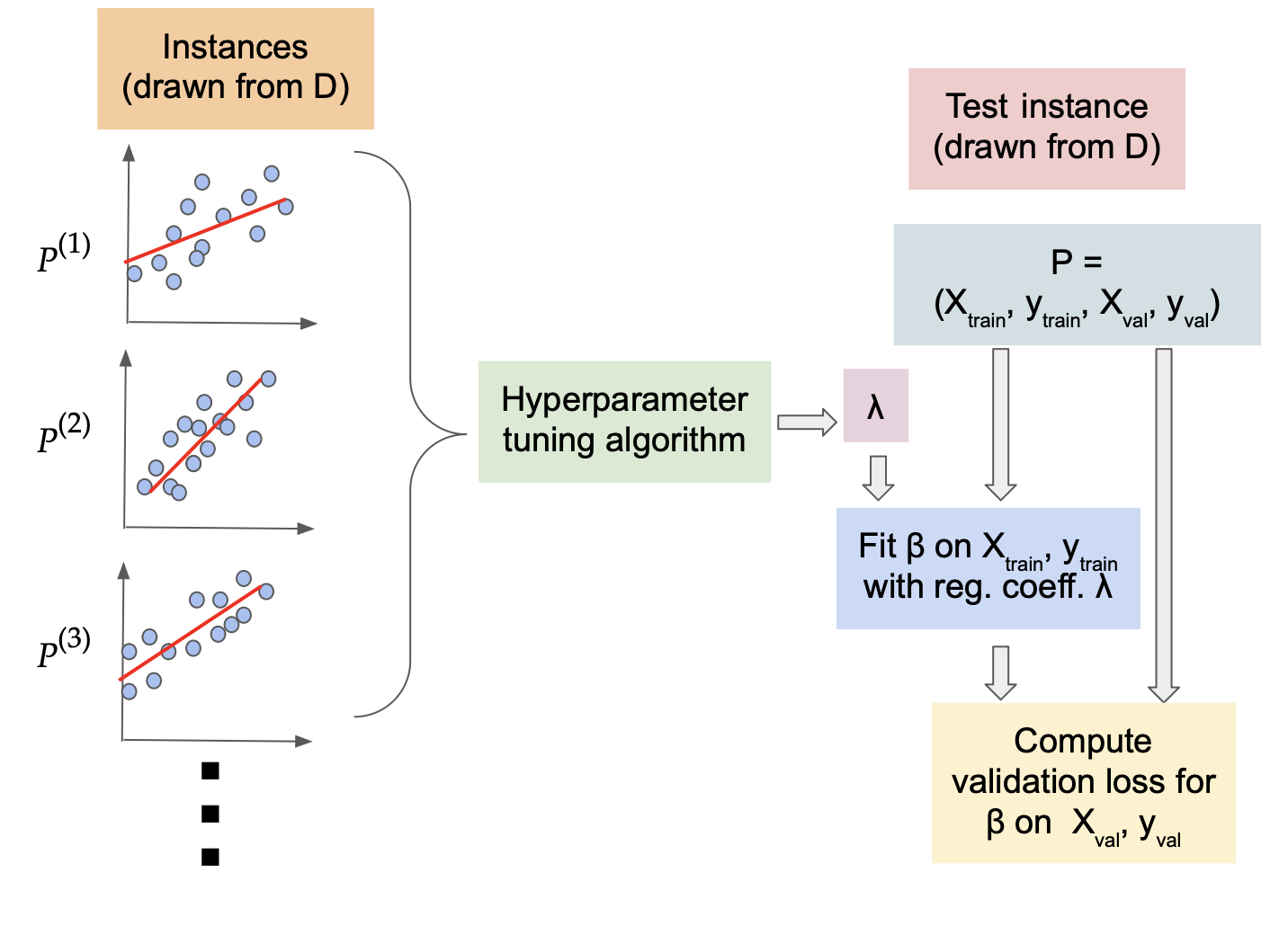
A series of regression instances in a pharmaceutical application. Can we learn how to set the regularization parameter (lambda) from similar domain-specific data?
Overview. Perhaps the simplest relation between a real dependent variable (y) and a vector of features (X) is a linear model (y = beta X). Given some training examples or datapoints consisting of pairs of features and dependent variables ((X_1, y_1),(X_2, y_2),dots,(X_m,y_m)), we would like to learn (beta) which would give the best prediction (y’) given features (X’) of an unseen example. This process of fitting a linear model (beta) to the datapoints is called linear regression. This simple yet effective model finds ubiquitous applications, ranging from biological, behavioral, and social sciences to environmental studies and financial forecasting, to make reliable predictions on future data. In ML terminology, linear regression is a supervised learning algorithm with low variance and good generalization properties. It is much less data-hungry than typical deep learning models, and performs well even with small amounts of training data. Further, to avoid overfitting the model to the training data, which reduces the prediction performance on unseen data, one typically uses regularization, which modifies the objective function of the linear model to reduce impact of outliers and irrelevant features (read on for details).
The most common method for linear regression is “regularized least squares”, where one finds the (beta) which minimizes
$$||y – beta X||_2^2 + lambda ||beta||.$$
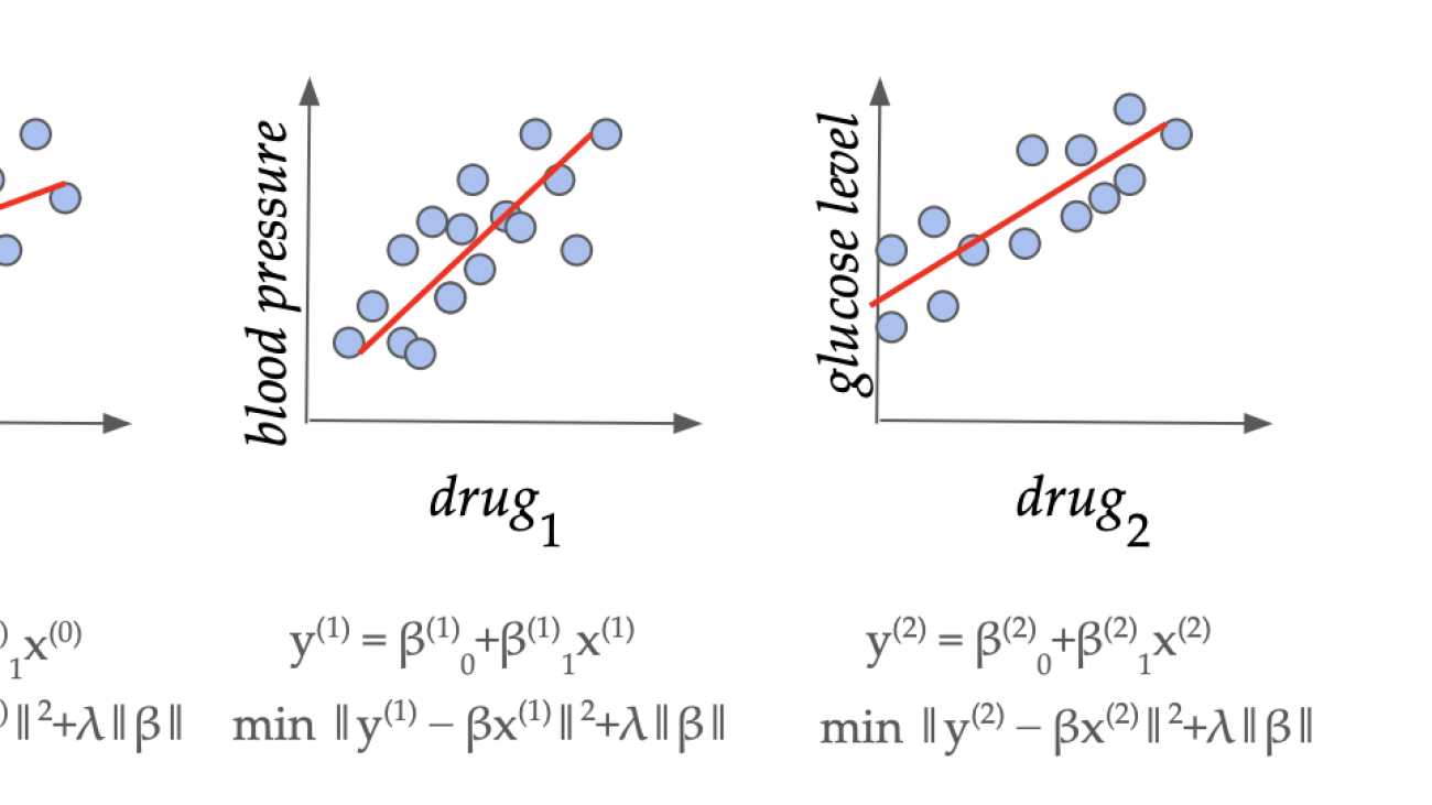
Here the first term captures the error of (beta) on the training set, and the second term is a norm-based penalty to avoid overfitting (e.g. reducing impact of outliers in data). How to set (lambda) appropriately in this fundamental method depends on the data domain and is a longstanding open question. In typical modern applications, we have access to several similar datasets (X^{(0)},y^{(0)}, X^{(1)},y^{(1)}, dots) from the same application domain. For example, there are often multiple drug trial studies in a pharmaceutical company for studying the different effects of similar drugs. In this work, we show that we can indeed learn a good domain-specific value of (lambda) with strong theoretical guarantees of accuracy on unseen datasets from the same domain, and give bounds on how much data is needed to achieve this.
As our main result, we show that if the data has (p) features (i.e., the dimension of feature vector (X_i) is (p), then after seeing (O(p/epsilon^2)) datasets, we can learn a value of (lambda) which has error (averaged over the domain) within (epsilon) of the best possible value of (lambda) for the domain. We also extend our results to sequential data, binary classification (i.e. (y) is binary valued) and non-linear regression.
Problem Setup. Linear regression with norm-based regularization penalty is one of the most popular techniques that one encounters in introductory courses to statistics or machine learning. It is widely used for data analysis and feature selection, with numerous applications including medicine, quantitative finance (the linear factor model), climate science, and so on. The regularization penalty is typically a weighted additive term (or terms) of the norms of the learned linear model (beta), where the weight is carefully selected by a domain expert. Mathematically, a dataset has dependent variable (y) consisting of (m) examples, and predictor variables (X) with (p) features for each of the (m) datapoints. The linear regression approach (with squared loss) consists of solving a minimization problem
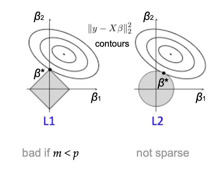
where the highlighted term is the regularization penalty. Here (lambda_1, lambda_2ge 0) are the regularization coefficients constraining the L1 and L2 norms, respectively, of the learned linear model (beta). For general (lambda_1) and (lambda_2) the above algorithm is popularly known as the Elastic Net, while setting (lambda_1 = 0) recovers Ridge regression and setting (lambda_2 = 0) corresponds to LASSO. Ridge and LASSO regression are both individually popular methods in practice, and the Elastic Net incorporates the advantages of both.
Despite the central role these coefficients play in linear regression, the problem of setting them in a principled way has been a challenging open problem for several decades. In practice, one typically uses “grid search” cross-validation, which involves (1) splitting the dataset into several subsets consisting of training and validation sets, (2) training several models (corresponding to different values of regularization coefficients) on each training set, and (3) comparing the performance of the models on the corresponding validation sets. This approach has several limitations.
First, this is very computationally intensive, especially with the large datasets that typical modern applications involve, as one needs to train and evaluate the model for a large number of hyperparameter values and training-validation splits. We would like to avoid repeating this cumbersome process for similar applications.
Second, theoretical guarantees on how well the coefficients learned by this procedure will perform on unseen examples are not known, even when the test data are drawn from the same distribution as the training set.
Finally, this can only be done for a finite set of hyperparameter values and it is not clear how the selected parameter compares to the best parameter from the continuous domain of coefficients. In particular, the loss as a function of the regularization parameter is not known to be Lipschitz.
Our work addresses all three of the above limitations simultaneously in the data-driven setting, which we motivate and describe next.
The importance of regularization
A visualization of the L1 and L2 regularized regressions.
The regularization coefficients (lambda_1) and (lambda_2) play a crucial role across fields: In machine learning, controlling the norm of model weights (beta) implies provable generalization guarantees and prevents over-fitting in practice. In statistical data analysis, their combined use yields parsimonious and interpretable models. In Bayesian statistics they correspond to imposing specific priors on (beta). Effectively, (lambda_2) regularizes (beta) by uniformly shrinking all coefficients, while (lambda_1) encourages the model vector to be sparse. This means that while they do yield learning-theoretic and statistical benefits, setting them to be too high will cause models to under-fit to the data. The question of how to set the regularization coefficients becomes even more unclear in the case of the Elastic Net, as one must juggle trade-offs between sparsity, feature correlation, and bias when setting both (lambda_1) and (lambda_2) simultaneously.
The data-driven algorithm design paradigm
In many applications, one has access to not just a single dataset, but a large number of similar datasets coming from the same domain. This is increasingly true in the age of big data, where an increasing number of fields are recording and storing data for the purpose of pattern analysis. For example, a drug company typically conducts a large number of trials for a variety of different drugs. Similarly, a climate scientist monitors several different environmental variables and continuously collects new data. In such a scenario, can we exploit the similarity of the datasets to avoid doing cumbersome cross-validation each time we see a new dataset? This motivates the data-driven algorithm design setting, introduced in the theory of computing community by Gupta and Roughgarden as a tool for design and analysis of algorithms that work well on typical datasets from an application domain (as opposed to worst-case analysis). This approach has been successfully applied to several combinatorial problems including clustering, mixed integer programming, automated mechanism design, and graph-based semi-supervised learning (Balcan, 2020). We show how to apply this analytical paradigm to tuning the regularization parameters in linear regression, extending the scope of its application beyond combinatorial problems [1, 2].
The learning model
A model for studying repeated regression instances from the same domain.
Formally, we model data coming from the same domain as a fixed (but unknown) distribution (D) over the problem instances. To capture the well-known cross-validation setting, we consider each problem instance of the form (P=(X_{text{train}}, y_{text{train}}, X_{text{val}}, y_{text{val}})). That is, the random process that generates the datasets and the (random or deterministic) process that generates the splits given the data, have been combined under (D). The goal of the learning process is to take (N) problem samples generated from the distribution (D), and learn regularization coefficients (hat{lambda}=(lambda_1, lambda_2)) that would generalize well over unseen problem instances drawn from (D). That is, on an unseen test instance (P’=(X’_{text{train}}, y’_{text{train}}, X’_{text{val}}, y’_{text{val}})), we will fit the model (beta) using the learning regularization coefficients (hat{lambda}) on (X’_{text{train}}, y’_{text{train}}), and evaluate the loss on the set (X’_{text{val}}, y’_{text{val}}). We seek the value of (hat{lambda}) that minimizes this loss, in expectation over the draw of the random test sample from (D).
How much data do we need?
The model (beta) clearly depends on both the dataset ((X,y)), and the regularization coefficients (lambda_1, lambda_2). A key tool in data-driven algorithm design is the analysis of the “dual function”, which is the loss expressed as a function of the parameters, for a fixed problem instance. This is typically easier to analyze than the “primal function” (loss for a fixed parameter, as problem instances are varied) in data-driven algorithm design problems. For Elastic Net regression, the dual is the validation loss on a fixed validation set for models trained with different values of (lambda_1, lambda_2) (i.e. two-parameter function) for a fixed training set. Typically the dual functions in combinatorial problems exhibit a piecewise structure, where the behavior of the loss function can have sharp transitions across the pieces. For example, in clustering this piecewise behavior could correspond to learning a different cluster in each piece. Prior research has shown that if we can bound the complexity of the boundary and piece functions in the dual function, then we can give a sample complexity guarantee, i.e. we can answer the question “how much data is sufficient to learn a good value of the parameter?”
An illustration of the piecewise structure of the Elastic Net dual loss function. Here (r_1) and (r_2) are polynomial boundary functions, and (f_{*,*}) are piece functions which are fixed rational functions given the signs of boundary functions.
Somewhat surprisingly, we show that the dual loss function exhibits a piecewise structure even in linear regression, a classic continuous optimization problem. Intuitively, the pieces correspond to different subsets of the features being “active”, i.e. having non-zero coefficients in the learned model (beta). Specifically, we show that the piece boundaries of the dual function are polynomial functions of bounded degree, and the loss within each piece is a rational function (ratio of two polynomial functions) again of bounded degree. We use this structure to establish a bound on the learning-theoretic complexity of the dual function; more precisely, we bound its pseudo-dimension (a generalization of the VC dimension to real-valued functions).
Theorem. The pseudo-dimension of the Elastic Net dual loss function is (Theta(p)), where (p) is the feature dimension.
(Theta(p)) notation here means we have an upper bound of (O(p)) as well as a lower bound (Omega(p)) on the pseudo-dimension. Roughly speaking, the pseudo-dimension captures the complexity of the function class from a learning perspective, and corresponds to the number of samples needed to guarantee small generalization error (average error on test data). Remarkably, we show an asymptotically tight bound on the pseudo-dimension by establishing a (Omega(p)) lower bound which is technically challenging and needs an explicit construction of a collection of “hard” instances. Tight lower bounds are not known for several typical problems in data-driven algorithm design. Our bound depends only on (p) (the number of features) and is independent of the number of datapoints (m). An immediate consequence of our bound is the following sample complexity guarantee:
Theorem. Given any distribution (D) (fixed, but unknown), we can learn regularization parameters (hat{lambda}) which obtain error within any (epsilon>0) of the best possible parameter with probability (1-delta) using only (O(1/epsilon^2(p+log 1/delta))) problem samples.
One way to understand our results is to instantiate them in the cross-validation setting. Consider the commonly used techniques of leave-one-out cross validation (LOOCV) and Monte Carlo cross validation (repeated random test-validation splits, typically independent and in a fixed proportion). Given a dataset of size (m_{text{tr}}), LOOCV would require (m_{text{tr}}) regression fits which can be computationally expensive for large datasets. Alternately, we can consider draws from a distribution (D_{text{LOO}}) which generates problem instances P from a fixed dataset ((X, y) in R^{m+1times p} times R^{m+1}) by uniformly selecting (j in [m + 1]) and setting (P = (X_{−j∗}, y_{−j} , X_{j∗}, y_j )). Our result now implies that roughly (O(p/epsilon^2)) iterations are enough to determine an Elastic Net parameter (hat{lambda}) with loss within (epsilon) (with high probability) of the parameter (lambda^*) obtained from running the full LOOCV. Similarly, we can define a distribution (D_{text{MC}}) to capture the Monte Carlo cross validation procedure and determine the number of iterations sufficient to get an (epsilon)-approximation of the loss corresponding parameter selection with an arbitrarily large number of runs. Thus, in a very precise sense, our results answer the question of how much cross-validation is enough to effectively implement the above techniques.
Sequential data and online learning
A more challenging variant of the problem assumes that the problem instances arrive sequentially, and we need to set the parameter for each instance using only the previously seen instances. We can think of this as a game between an online adversary and the learner, where the adversary wants to make the sequence of problems as hard as possible. Note that we no longer assume that the problem instances are drawn from a fixed distribution, and this setting allows problem instances to depend on previously seen instances which is typically more realistic (even if there is no actual adversary generating worst-case problem sequences). The learner’s goal is to perform as well as the best fixed parameter in hindsight, and the difference is called the “regret” of the learner.
To obtain positive results, we make a mild assumption on the smoothness of the data: we assume that the prediction values (y) are drawn from a bounded density distribution. This captures a common data pre-processing step of adding a small amount of uniform noise to the data for model stability, e.g. by setting the jitter parameter in the popular Python library scikit-learn. Under this assumption, we show further structure on the dual loss function. Roughly speaking, we show that the location of the piece boundaries of the dual function across the problem instances do not concentrate in a small region of the parameter space.This in turn implies (using Balcan et al., 2018) the existence of an online learner with average expected regret (O(1/sqrt{T})), meaning that we converge to the performance of the best fixed parameter in hindsight as the number of online rounds (T) increases.
Extension to binary classification, including logistic regression
Linear classifiers are also popular for the task of binary classification, where the (y) values are now restricted to (0) or (1). Regularization is also crucial here to learn effective models by avoiding overfitting and selecting important variables. It is particularly common to use logistic regression, where the squared loss above is replaced by the logistic loss function,
The exact loss minimization problem is significantly more challenging in this case, and it is correspondingly difficult to analyze the dual loss function. We overcome this challenge by using a proxy dual function which approximates the true loss function, but has a simpler piecewise structure. Roughly speaking, the proxy function considers a fine parameter grid of width (epsilon) and approximates the loss function at each point on the grid. Furthermore, it is piecewise linear and known to approximate the true loss function to within an error of (O(epsilon^2)) at all points (Rosset, 2004).
Our main result for logistic regression is that the generalization error with (N) samples drawn from the distribution (D) is bounded by (O(sqrt{(m^2+log 1/epsilon)/N}+epsilon^2+sqrt{(log 1/delta)/N})), with (high) probability (1-delta) over the draw of samples. (m) here is the size of the validation set, which is often small or even constant. While this bound is incomparable to the pseudo-dimension-based bounds above, we do not have lower bounds in this setting and tightness of our results in an interesting open question.
So far, we have assumed that the dependent variable (y) has a linear dependence on the predictor variables. While this is a great first thing to try in many applications, very often there is a non-linear relationship between the variables. As a result, linear regression can result in poor performance in some applications. A common alternative is to use Kernelized Least Squares Regression, where the input (X) is implicitly mapped to high (or even infinite) dimensional feature space using the “kernel trick”. As a corollary of our main results, we can show that the pseudo-dimension of the dual loss function in this case is (O(m)), where (m) is the size of the training set in a single problem instance. Our results do not make any assumptions on the (m) samples within a problem instance/dataset; if these samples within problem instances are further assumed to be i.i.d. draws from some data distribution (distinct from problem distribution (D)), then well-known results imply that (m = O(k log p)) samples are sufficient to learn the optimal LASSO coefficient ((k) denotes the number of non-zero coefficients in the optimal regression fit).
Some final remarks
We consider how to tune the norm-based regularization parameters in linear regression. We pin down the learning-theoretic complexity of the loss function, which may be of independent interest. Our results extend to online learning, linear classification, and kernel regression. A key direction for future research is developing an efficient implementation of the algorithms underlying our approach.
More broadly, regularization is a fundamental technique in machine learning, including deep learning where it can take the form of dropout rates, or parameters in the loss function, with significant impact on the performance of the overall algorithm. Our research opens up the exciting question of tuning learnable parameters even in continuous optimization problems. Finally, our research captures an increasingly typical scenario with the advent of the data era, where one has access to repeated instances of data from the same application domain.
For further details about our cool results and the mathematical machinery we used to derive them, check out our papers linked below!
TL;DR: Off-the-shelf text spotting and re-identification models fail in basic off-road racing settings, even more so during muddy events. Making matters worse, there aren’t any public datasets to tune or improve models in this domain. To this end, we introduce datasets, benchmarks, and methods for the challenging off-road racing setting.
In the dynamic world of sports analytics, machine learning (ML) systems play a pivotal role, transforming vast arrays of visual data into actionable insights. These systems are adept at navigating through thousands of photos to tag athletes, enabling fans and participants alike to swiftly locate images of specific racers or moments from events. This technology has seamlessly integrated intovarioussports, significantly enhancing the spectator experience and operational efficiency. Yet, not all sports environments cater equally to the capabilities of current ML models. Off-road motorcycle racing, characterized by its unpredictable and untamed wilderness settings, poses unique challenges that push the boundaries of what existing computer vision systems can handle.
Imagine the conditions under which off-road races are conducted: racers blitz through waist-deep mud holes, endure torrential rains, navigate through blinding dust clouds, and much more. Such extreme environmental factors introduce variables like mud occlusion, complex poses (racers frequently crash), glare, motion blur, and variable lighting conditions, which significantly degrade the performance of conventional text spotting and person re-identification (ReID) models. Typical models, trained on more ‘sterile’ conditions, falter when faced with the task of identifying racers and their numbers in the chaotic and mud-splattered scenes typical of off-road racing events. Take, for example, these images of the same racer, taken only minutes apart:
Figure 1: Four images of a single racer taken during the same event. Accurately matching a rider throughout the event is extremely difficult due to the very high variation in appearance caused by mud, odd poses, and much more.
The lack of public datasets tailored to these rugged conditions exacerbates the problem, leaving researchers and practitioners without the resources needed to tune and enhance models for better performance in off-road racing, or equally unconstrained, scenarios. Recognizing this gap, our work aims to bridge it by introducing new datasets and benchmarks specifically designed for the challenging setting of off-road motorcycle racing. This blog post will delve into the unique challenges presented by off-road racing environments, describe our efforts in creating datasets that capture these conditions, and discuss methods and benchmarks for improving computer vision models to robustly handle the extreme variability inherent in off-road racing. I’ll even give a brief overview of some new weakly supervised methods for improving models in these challenging areas, with very little labeled data. Join in as we explore the uncharted territories of machine learning applications in off-road motorcycle racing, pushing the limits of what’s possible in sports analytics and beyond.
The Challenges
Figure 2: More examples of the challenging conditions presented by off-road racing, causing the performance of existing models and methods to fall below an acceptable threshold.
Off-road motorcycle racing is an adrenaline-pumping sport that takes athletes and their machines through some of the most challenging terrains nature have to offer. Unlike the relatively predictable environments of track racing or urban marathons, off-road racing is fraught with unpredictability and extreme conditions. The very essence of what makes it thrilling for participants and spectators alike—mud, dust, water, uneven terrain—presents a formidable challenge for computer vision systems. Here, we delve into the specific hurdles that these conditions pose for text spotting and re-identification models in off-road racing scenarios.
Dirt is pervasive in off-road racing, manifesting itself as mud or dust. As races progress, vehicles and riders become increasingly coated in dirt, which can obscure critical identifying features such as racer numbers or distinguishing gear colors. The dynamic nature of off-road racing means that athletes are rarely in simple, upright poses. Instead, they navigate the course through jumps, sharp turns, and even crashes. The outdoor settings of off-road races often move rapidly from deep dark forests to bright glaring fields, thus introducing variable lighting conditions. Similarly, the high speeds at which racers move combined with the stylistic choices of some photographers can lead to motion blur. In each of these cases, traditional (OCR) and re-identification (ReID) models, trained primarily on clean, unobstructed images, struggle to recognize text or identify individuals.
The Datasets and Initial Benchmarks
To tackle the formidable challenges presented by off-road motorcycle racing, we embarked on a mission to create and introduce datasets that accurately capture the essence and extremities of this sport. Recognizing the gap in existing computer vision resources, our datasets—off-road Racer Number Dataset (RND) and MUddy Racer re-iDentification Dataset (MUDD)—are meticulously curated to serve as a robust foundation for developing and benchmarking models capable of operating in the harsh, unpredictable conditions of off-road racing. These datasets, as well as benchmarking code, are publically available for both of these datasets. You can find RND here and MUDD here.
Figure 3 details the text spotting results on the RND dataset. Results are broken down by the various types of occlusion in the dataset. Even on the cleanest data (i.e. the data with no occlusion), the best fine-tuned models reach a maximum E2E F1 score of 0.6, leaving a lot to be desired. Introducing any of the aforementioned challenges (i.e.) reduces this even further, down to the worse end-to-end F1 score of 0.29. The models tested were the Yet Another Mask Text Spotter (YAMTS) and Swin Text Spotter, and YAMTS was consistently the best performing. Fine-tuning reduces the negative effect of the various occlusion types (i.e. the blue bar changes less as a percentage of performance than the orange across the various occlusions), yet occlusion still causes significant performance degradation.
Figure 3: Text Detection and Recognition results on the RND dataset (higher is better). Results are broken down by the types of occlusion present in the data. The left plot details the detection performance, whereas the right plot details the end-to-end text recognition F1 score, where a prediction is correct only if the detection and predicted text match exactly. While vanilla fine-tuning helps a lot and reduces the negative effects of occlusion, mud still remains an unsolved challenge. More advancements are needed for high performing off-road racing OCR techniques.
Figure 4 breaks down the performance of our best ReID models. In the standard ReID evaluation setting, a sample from a query set is used to return a ranking over a gallery set. We report the rank1 accuracy along with the mean average precision (mAP). Figure 2 looks at two variations of the query and gallery sets, one query set of all the muddy images, and one without, and the same for the gallery set. In the simplest setting (No Mud -> No Mud), model performance is getting reasonably good, around 0.9 mAP. However, mud drops this performance by as much as 30%. The models tested were the Omni-Scale Network (OSNet) and Resnet 50. Figure 4 reports results from OSNet as it was most performant.
Figure 4: Rank@1 accuracy and mean average precision (mAP) on the MUDD dataset. The query and gallery sets are broken into two groups based on the presence of mud. While the ReID model performs well among clean data, mud causes a performance drop of as much as 30%.
In summary, the off-road racing setting is difficult, even in the best case. Once dirt and mud enter the equation, models require advancement before they reach the threshold of usability in a real-world application.
Improving These Systems
A “Mud-Like” Data Augmentation
Figure 5: Examples of a new data augmentation strategy, referred to as speckling. The idea behind this is to imitate the “splotchy” nature of mud splatters. This data augmentation improves re-id and text spotting performance by 4% and 7% respectively.
The first step in building robustness to mud is to introduce a data augmentation strategy: speckling. As shown in previous examples, mud often accumulates in small chunks. To emulate this, we introduce speckling, where we randomly change many small patches of the input imagery into the pixel mean. This is similar to random erasing but at a much smaller scale with a large number of patches being erased in each image. This technique leads to a 4% improvement in Rank-1 accuracy for person re-identification on the MUDD dataset, and while it does not meaningfully affect the detection F1 score of text spotting on RND, it does improve the end-to-end F1 score by 7%. While we also use the standard color jitter data augmentation to help robustness to the color changes induced as a racer gets dirty, more research is needed to determine if a more specific color augmentation can prove useful.
Learning from Weak Labels
Another intricacy of sports imagery that we can take advantage of is the natural groupings that often exist. For example, prior marathon imagery has been manually grouped by humans, such that each group (which we will refer to as a bag) consists of images that all contain a specific individual. However, which specific individual is the one of interest in each image is unknown. In motorcycle racing, we have the same data, as well as customer purchase history. Most customers purchase photos of a single racer, therefore the list of purchased photos again becomes a bag of a specific individual, although which individuals in the image is unknown. This type of label is visualized in Figure 4.
Figure 6: Weakly labeled person re-identification. Each bag represents all crops of individuals in a group of photos, where each photo group is known to contain photos containing one specific individual. However, each photo also contains multiple people, and there is no way to tell which person in each image is the one of interest.
We introduce Contrastive Multiple Instance Learning (CMIL) to address this challenge. This method works by generating bag representations from all of the instance representations that comprise that bag. Then, the bag representations are used to optimize a model via triplet loss or classification loss. In other words, we optimize the model to accurately classify bags, not individuals. This does not align with our test time goal, however, of classifying individuals. But surprisingly, our bag classification models naturally generate useful individual representations. Figure 5 gives an overview of the CMIL model. On the MUDD dataset, CMIL improves over the next-best weakly labeledperson re-identification methodology by 4% rank-1 accuracy, and over a model that trusts the bag-level labels to be accurate person-level labels by over 20%.
Figure 7: The CMIL method which enables learning effective person (racer) re-identification models, even when only given data weakly labeled in bags as described in Figure 6. The key idea in making this possible is to compare bag embeddings instead of instance embeddings.
Conclusion
Off-road racing poses major challenges to existing text spotting and person re-identification methods and models, rendering them unfit for practical application. Our first steps at improving computer performance in these areas include introducing two datasets for the corresponding problems, introducing a new data augmentation technique, and bringing contrastive learning to the multiple instance learning framework. We hope that these initial works spur more innovation in off-road applications.
TLDR; Design biases in NLP systems, such as performance differences for different populations, often stem from their creator’s positionality, i.e., views and lived experiences shaped by identity and background. Despite the prevalence and risks of design biases, they are hard to quantify because researcher, system, and dataset positionality are often unobserved.
We introduce NLPositionality, a framework for characterizing design biases and quantifying the positionality of NLP datasets and models. We find that datasets and models align predominantly with Western, White, college-educated, and younger populations. Additionally, certain groups such as nonbinary people and non-native English speakers are further marginalized by datasets and models as they rank least in alignment across all tasks.
Figure 1. Carl from the U.S. and Aditya from India both want to use Perspective API, but it works better for Carl than it does for Aditya. This is because toxicity researchers’ positionalities lead them to make design choices that make toxicity datasets, and thus Perspective API, to have positionalities that are Western-centric.
Imagine the following scenario (see Figure 1): Carl, who works for the New York Times, and Aditya, who works for the Times of India, both want to use Perspective API. However, Perspective API fails to label instances containing derogatory terms in Indian contexts as “toxic”, leading it to work better overall for Carl than Aditya. This is because toxicity researchers’ positionalities lead them to make design choices that make toxicity datasets, and thus Perspective API, to have Western-centric positionalities.
In this study, we developed NLPositionality, a framework to quantify the positionalities of datasets and models. Prior work has introduced the concept of model positionality, defining it as “the social and cultural position of a model with regard to the stakeholders with which it interfaces.” We extend this definition to add that datasets also encode positionality, in a similar way as models. Thus, model and dataset positionality results in perspectives embedded within language technologies, making them less inclusive towards certain populations.
In this work, we highlight the importance of considering design biases in NLP. Our findings showcase the usefulness of our framework in quantifying dataset and model positionality. In a discussion of the implications of our results, we consider how positionality may manifest in other NLP tasks.
Figure 2. Overview of the NLPositionality Framework. Collection (steps 1-4): A subset of datasets’ instances are re-annotated via diverse volunteers recruited on LabintheWild. Processing (step 5): We compare the labels collected from LabintheWild with the dataset’s original labels and models’ predictions. Analysis (step 6): We compute the Pearson’s r correlation between the LabintheWild annotations by demographic for the dataset’s original labels and the models’ predictions. We apply the Bonferroni correction to account for multiple hypothesis testing.Figure 3. Example Annotation. An example instance from the Social Chemistry dataset that was sent to LabintheWild along with the mean of the received annotation scores across various demographics.
NLPositionality:Quantifying Dataset and Model Positionality
Our NLPositionality framework follows a two-step process for characterizing the design biases and positionality of datasets and models. We present an overview of the NLPositionality framework in Figure 2.
First, a subset of data for a task is re-annotated by annotators from around the world to obtain globally representative data in order to quantify positionality. An example of a reannotation is included in Figure 3. We perform reannotation for two tasks: hate speech detection (i.e., harmful speech targeting specific group characteristics) and social acceptability (i.e., how acceptable certain actions are in society). For hate speech detection, we study the DynaHate dataset along with the following models: Perspective API, Rewire API, ToxiGen RoBERTa, and GPT-4 zero shot. For social acceptability, we study the Social Chemistry dataset along with the following models: the Delphi model and GPT-4 zero shot.
Then, the positionality of the dataset or model is computed by calculating the Pearson’s r scores between responses of the dataset or model with the responses of different demographic groups for identical instances. These scores are then compared with one another to determine how models and datasets are biased.
While relying on demographics as a proxy for positionality is limited, we use demographic information for an initial exploration in uncovering design biases in datasets and models.
Table 1: Positionality of NLP datasets and models quantified using Pearson’s r correlation coefficients. # denotes the number of annotations associated with a demographic group. α denotes Krippendorff’s alpha of a demographic group for a task. * denotes statistical significance (p<2.04e−05 after Bonferroni correction). For each dataset or model, we denote the minimum and maximum Pearson’s r value for each demographic category in red and blue respectively.
The demographic groups collected from LabintheWild are represented as rows in the table; the Pearson’s r scores between the demographic groups’ labels and each model and/or dataset are located in the last three and five columns within the social acceptability and toxicity and hate speech sections respectively. For example, in the fifth row and the third column, there is the value 0.76. This indicates Social Chemistry has a Pearson’s r value of 0.76 with English-speaking countries, indicating a stronger correlation with this population.
Experimental Results
Our results are displayed in Table 1. Overall, across all tasks, models, and datasets, we find statistically significant moderate correlations with Western, educated, White, and young populations, indicating that language technologies are WEIRD (Western, Educated, Industrialized, Rich, Democratic) to an extent, though each to varying degrees. Also, certain demographics consistently rank lowest in their alignment with datasets and models across both tasks compared to other demographics of the same type.
Social acceptability. Social Chemistry is most aligned with people who grow up and live in English speaking countries, who have a college education, are White, and are 20-30 years old. Delphi also exhibits a similar pattern, but to a lesser degree. While it strongly aligns with people who grow up and live in English-speaking countries, who have a college education (r=0.66), are White, and are 20-30 years old. We also observe a similar pattern with GPT-4. It has the highest Pearson’s r value for people who grow up and live in English-speaking countries, are college-educated, are White and are between 20-30 years old.
Non-binary people align less to both Social Chemistry, Delphi, and GPT-4 compared to men and women. Black, Latinx, and Native American populations consistently rank least in correlation to education level and ethnicity.
Hate speech detection. Dynahate is highly correlated with people who grow up in English-speaking countries, who have a college education, are White, and are 20-30 years old. Perspective API also tends to align with WEIRD populations, though to a lesser degree than DynaHate. Perspective API exhibits some alignment with people who grow up and live in English-speaking, have a college education, are White, and are 20-30 years old. Rewire API similarly shows this bias. It has a moderate correlation with people who grow up and live in English-speaking countries, have a college education, are White, and are 20-30 years old. A Western bias is also shown in ToxiGen RoBERTa. ToxiGen RoBERTa shows some alignment with people who grow up and live in English-speaking countries, have a college education, are White and are between 20-30 years of age. We also observe similar behavior with GPT-4. The demographics with some of the higher Pearson’s r values in its category are people who grow up and live in English-speaking countries, are college-educated, are White, and are 20-30 years old. It shows stronger alignment with Asian-Americans compared to White people.
Non-binary people align less with Dynahate, PerspectiveAPI, Rewire API, ToxiGen RoBERTa, andGPT-4 compared to other genders. Also, people are Black, Latinx, and NativeAmerican rank least in alignment for education and ethnicity respectively.
What can we do about dataset and model positionality?
Based on these findings, we have recommendations for researchers on how to handle dataset and model positionality:
Keep a record of all design choices made while building datasets and models. This can improve reproducibility and aid others in understanding the rationale behind the decisions, revealing some of the researcher’s positionality.
Report your positionality and the assumptions you make.
Use methods to center the perspectives of communities who are harmed by design biases. This can be done using approaches such as participatory design as well as value-sensitive design.
Make concerted efforts to recruit annotators from diverse backgrounds. Since new design biases could be introduced in this process, we recommend following the practice of documenting the demographics of annotators to record a dataset’s positionality.
Be mindful of different perspectives by sharing datasets with disaggregated annotations and finding modeling techniques that can handle inherent disagreements or distributions, instead of forcing a single answer in the data.
Finally, we argue that the notion of “inclusive NLP” does not mean that all language technologies have to work for everyone. Specialized datasets and models are immensely valuable when the data collection process and other design choices are intentional and made to uplift minority voices or historically underrepresented cultures and languages, such as Masakhane-NER and AfroLM.
Evaluating models in federated networks is challenging due to factors such as client subsampling, data heterogeneity, and privacy. These factors introduce noise that can affect hyperparameter tuning algorithms and lead to suboptimal model selection.
Hyperparameter tuning is critical to the success of cross-device federated learning applications. Unfortunately, federated networks face issues of scale, heterogeneity, and privacy, which introduce noise in the tuning process and make it difficult to faithfully evaluate the performance of various hyperparameters. Our work (MLSys’23) explores key sources of noise and surprisingly shows that even small amounts of noise can have a significant impact on tuning methods—reducing the performance of state-of-the-art approaches to that of naive baselines. To address noisy evaluation in such scenarios, we propose a simple and effective approach that leverages public proxy data to boost the evaluation signal. Our work establishes general challenges, baselines, and best practices for future work in federated hyperparameter tuning.
Federated Learning: An Overview
In federated learning (FL), user data remains on the device and only model updates are communicated. (Source: Wikipedia)
Cross-device federated learning (FL) is a machine learning setting that considers training a model over a large heterogeneous network of devices such as mobile phones or wearables. Three key factors differentiate FL from traditional centralized learning and distributed learning:
Scale. Cross-device refers to FL settings with many clients with potentially limited local resources e.g. training a language model across hundreds to millions of mobile phones. These devices have various resource constraints, such as limited upload speed, number of local examples, or computational capability.
Heterogeneity. Traditional distributed ML assumes each worker/client has a random (identically distributed) sample of the training data. In contrast, in FL client datasets may be non-identically distributed, with each user’s data being generated by a distinct underlying distribution.
Privacy. FL offers a baseline level of privacy since raw user data remains local on each client. However, FL is still vulnerable to post-hoc attacks where the public output of the FL algorithm (e.g. a model or its hyperparameters) can be reverse-engineered and leak private user information. A common approach to mitigate such vulnerabilities is to use differential privacy, which aims to mask the contribution of each client. However, differential privacy introduces noise in the aggregate evaluation signal, which can make it difficult to effectively select models.
Federated Hyperparameter Tuning
Appropriately selecting hyperparameters (HPs) is critical to training quality models in FL. Hyperparameters are user-specified parameters that dictate the process of model training such as the learning rate, local batch size, and number of clients sampled at each round. The problem of tuning HPs is general to machine learning (not just FL). Given an HP search space and search budget, HP tuning methods aim to find a configuration in the search space that optimizes some measure of quality within a constrained budget.
Let’s first look at an end-to-end FL pipeline that considers both the processes of training and hyperparameter tuning. In cross-device FL, we split the clients into two pools for training and validation. Given a hyperparameter configuration ((lambda_s, lambda_c)), we train a model using the training clients (explained in section “FL Training”). We then evaluate this model on the validation clients, obtaining an error rate/accuracy metric. We can then use the error rate to adjust the hyperparameters and train a new model.
A standard pipeline for tuning hyperparameters in cross-device FL.
The diagram above shows two vectors of hyperparameters (lambda_s, lambda_c). These correspond to the hyperparameters of two optimizers: one is server-side and the other is client-side. Next, we describe how these hyperparameters are used during FL training.
FL Training
A typical FL algorithm consists of several rounds of training where each client performs local training followed by aggregation of the client updates. In our work, we experiment with a general framework called FedOPT which was presented in Adaptive Federated Optimization (Reddi et al. 2021). We outline the per-round procedure of FedOPT below:
The server broadcasts the model (theta) to a sampled subset of (K) clients.
Each client (in parallel) trains (theta) on their local data (X_k) using ClientOPTand obtains an updated model (theta_k).
Each client sends (theta_k) back to the server.
The server averages all the received models \(theta’ = frac{1}{K} sum_k p_ktheta_k).
To update (theta), the server computes the difference (theta – theta’) and feeds it as a pseudo-gradient into ServerOPT (rather than computing a gradient w.r.t. some loss function).
The FedOPT framework and the five hyperparameters ((lambda_s, lambda_c)) we consider tuning. (Source: edited from Wikipedia)
Steps 2 and 5 of FedOPT each require a gradient-based optimization algorithm (called ClientOPT and ServerOPT) which specify how to update (theta) given some update vector. In our work, we focus on an instantiation of FedOPT called FedAdam, which uses Adam (Kingma and Ba 2014) as ServerOPT and SGD as ClientOPT. We focus on tuning five FedAdam hyperparameters: two for client training (SGD’s learning rate and batch size) and three for server aggregation (Adam’s learning rate, 1st-moment decay, and 2nd-moment decay).
FL Evaluation
Now, we discuss how FL settings introduce noise to model evaluation. Consider the following example below. We have (K=4) configurations (grey, blue, red, green) and we want to figure out which configuration has the best average accuracy across (N=5) clients. More specifically, each “configuration” is a set of HP values (learning rate, batch size, etc.) that are fed into an FL training algorithm (more details in the next section). This produces a model we can evaluate. If we can evaluate every model on every client then our evaluation is noiseless. In this case, we would be able to accurately determine that the green model performs the best. However, generating all the evaluations as shown below is not practical, as evaluation costs scale with both the number of configurations and clients.
HP tuning without noise. Every configuration is evaluated on every client, which allows us to find the best (green) configuration.
Below, we show an evaluation procedure that is more realistic in FL. As the primary challenge in cross-device FL is scale, we evaluate models using only a random subsample of clients. This is shown in the figure by red ‘X’s and shaded-out phones. We cover three additional sources of noise in FL which can negatively interact with subsampling and introduce even more noise into the evaluation procedure:
Data heterogeneity. FL clients may have non-identically distributed data, meaning that the evaluations on various models can differ between clients. This is shown by the different histograms next to each client. Data heterogeneity is intrinsic to FL and is critical for our observations on noisy evaluation; if all clients had identical datasets, there would be no need to sample more than one client.
Systems heterogeneity. In addition to data heterogeneity, clients may have heterogeneous system capabilities. For example, some clients have better network reception and computational hardware, which allows them to participate in training and evaluation more frequently. This biases performance towards these clients, leading to a poor overall model.
Differential privacy. Using the evaluation output (i.e. the top-performing model), a malicious party can infer whether or not a particular client participated in the FL procedure. At a high level, differential privacy aims to mask user contributions by adding noise to the aggregate evaluation metric. However, this additional noise can make it difficult to faithfully evaluate HP configurations.
In the figure above, evaluations can lead to suboptimal model selection when we consider client subsampling, data heterogeneity, and differential privacy. The combination of all these factors leads us to incorrectly choose the red model over the green one.
Experimental Results
The first goal of our work is to investigate the impact of four sources of noisy evaluation that we outlined in the section “FL Evaluation”. In more detail, these are our research questions:
How does subsampling validation clients affect HP tuning performance?
How do the following factors interact with/exacerbate issues of subsampling?
data heterogeneity (shuffling validation clients’ datasets)
systems heterogeneity (biased client subsampling)
privacy (adding Laplace noise to the aggregate evaluation)
In noisy settings, how do SOTA methods compare to simple baselines?
Surprisingly, we show that state-of-the-art HP tuning methods can perform catastrophically poorly, even worse than simple baselines (e.g., random search). While we only show results for CIFAR10, results on three other datasets (FEMNIST, StackOverflow, and Reddit) can be found in our paper. CIFAR10 is partitioned such that each client has at most two out of the ten total labels.
Noise hurts random search
This section investigates questions 1 and 2 using random search (RS) as the hyperparameter tuning method. RS is a simple baseline that randomly samples several HP configurations, trains a model for each one, and returns the highest-performing model (i.e. the example in “FL Evaluation”, if the configurations were sampled independently from the same distribution). Generally, each hyperparameter value is sampled from a (log) uniform or normal distribution.
Random search with varying only client subsampling (left) and varying both client subsampling and data heterogeneity (right).
Client subsampling. We run RS while varying the client subsampling rate from a single client to the full validation client pool. “Best HPs” indicates the best HPs found across all trials of RS. As we subsample less clients (left), random search performs worse (higher error rate).
Data heterogeneity. We run RS on three separate validation partitions with varying degrees of data heterogeneity based on the label distributions on each client. Client subsampling generally harms performance but has a greater impact on performance when the data is heterogeneous (IID Fraction = 0 vs. 1).
Random search with varying systems heterogeneity (left) and privacy budget (right). Both factors interact negatively with client subsampling.
Systems heterogeneity. We run RS and bias the client sampling to reflect four degrees of systems heterogeneity. Based on the model that is currently being evaluated, we assign a higher probability of sampling clients who perform well on this model. Sampling bias leads to worse performance since the biased evaluations are overly optimistic and do not reflect performance over the entire validation pool.
Privacy. We run RS with 5 different evaluation privacy budgets (varepsilon). We add noise sampled from (text{Lap}(M/(varepsilon |S|))) to the aggregate evaluation, where (M) is the number of evaluations (16), (varepsilon) is the privacy budget (each curve), and (|S|) is the number of clients sampled for an evaluation (x-axis). A smaller privacy budget requires sampling a larger raw number of clients to achieve reasonable performance.
Noise hurts complex methods more than RS
Seeing that noise adversely affects random search, we now focus on question 3: Do the same observations hold for more complex tuning methods? In the next experiment, we compare 4 representative HP tuning methods.
Tree-Structured Parzen Estimator (TPE) is a selection-based method. These methods build a surrogate model that predicts the performance of various hyperparameters rather than predictions for the task at hand (e.g. image or language data).
Hyperband (HB) is an allocation-based method. These methods allocate more resources to the most promising configurations. Hyperband initially samples a large number of configurations but stops training most of them after the first few rounds.
Examples of (a) selection-based and (b) allocation-based HP tuning methods. (a) uses a surrogate model of the search space to sample the next configuration (numbered in order of exploration), while (b) randomly samples many configurations and adaptively allocates resources to the most promising ones. (Source: Hyperband (Li et al. 2018))
We report the error rate of each HP tuning method (y-axis) at a given budget of rounds (x-axis). Surprisingly, we find that the relative ranking of these methods can be reversed when the evaluation is noisy. With noise, the performance of all methods degrades, but the degradation is particularly extreme for HB and BOHB. Intuitively, this is because these two methods already inject noise into the HP tuning procedure via early stopping which interacts poorly with additional sources of noise. Therefore, these results indicate a need for HP tuning methods that are specialized for FL, as many of the guiding principles for traditional hyperparameter tuning may not be effective at handling noisy evaluation in FL.
We compare 4 HP tuning methods in noiseless vs. noisy FL settings. In the noiseless setting (left), we always sample all the validation clients and do not consider privacy. In the noisy setting (right), we sample 1% of validation clients and have a generous privacy budget of (varepsilon=100).
Proxy evaluation outperforms noisy evaluation
In practical FL settings, a practitioner may have access to public proxy data which can be used to train models and select hyperparameters. However, given two distinct datasets, it is unclear how well hyperparameters can transfer between them. First, we explore the effectiveness of hyperparameter transfer between four datasets. Below, we see that the CIFAR10-FEMNIST and StackOverflow-Reddit pairs (top left, bottom right) show the clearest transfer between the two datasets. One likely reason for this is that these task pairs use the same model architecture: CIFAR10 and FEMNIST are both image classification tasks while StackOverflow and Reddit are next-word prediction tasks.
We experimented with 4 datasets in our work (CIFAR10, FEMNIST, StackOverflow, and Reddit). For each pair of datasets, we randomly sample 128 configurations and plot each configuration at the coordinates corresponding to the error rate on the two datasets.
Given the appropriate proxy dataset, we show that a simple method called one-shot proxy random search can perform extremely well. The algorithm has two steps:
Run a random search using the proxy data to both train and evaluate HPs. We assume the proxy data is both public and server-side, so we can always evaluate HPs without subsampling clients or adding privacy noise.
The output configuration from 1. is used to train a model on the training client data. Since we pass only a single configuration to this step, validation client datadoes not affect hyperparameter selection at all.
In each experiment, we choose one of these datasets to be partitioned among the clients and use the other three datasets as server-side proxy datasets. Our results show that proxy data can be an effective solution.Even if the proxy dataset is not an ideal match for the public data, it may be the only available solution under a strict privacy budget. This is shown in the FEMNIST plot where the orange/red lines (text datasets) perform similarly to the (varepsilon=10) curve.
We compare tuning HPs using noisy evaluations on the private dataset (with 1% client subsampling and varying the privacy budget (varepsilon) versus noiseless evaluations on the proxy dataset. The proxy HP tuning methods appear as horizontal lines because they are one-shot.
Conclusion
In conclusion, our study suggests several best practices for federated HP tuning:
Use simple HP tuning methods.
Sample a sufficiently large number of validation clients.
Evaluate a representative set of clients.
If available, proxy data can be an effective solution.
Furthermore, we identify several directions for future work in federated HP tuning:
Tailoring HP tuning methods for differential privacy and FL. Early stopping methods are inherently noisy/biased and the large number of evaluations they use is at odds with privacy. Another useful direction is to investigate HP methods specific to noisy evaluation.
More detailed cost evaluation. In our work, we only considered the number of training rounds as our resource budget. However, practical FL settings consider a wide variety of costs, such as total communication, amount of local training, or total time to train a model.
Combining proxy and client data for HP tuning. A key issue of using public proxy data for HP tuning is that the best proxy dataset is not known in advance. One direction to address this is to design methods that combine public and private evaluations to mitigate bias from proxy data and noise from private data. Another promising direction is to rely on the abundance of public data and design a method that can select the best proxy dataset.
TLDR: We introduce RoboTool, enabling robots to use tools creatively with large language models, which solves long-horizon hybrid discrete-continuous planning problems with the environment- and embodiment-related constraints.
Tool use is an essential hallmark of advanced intelligence. Some animals can use tools to achieve goals that are infeasible without tools. For example, crows solve a complex physical puzzle using a series of tools, and apes use a tree branch to crack open nuts or fish termites with a stick. Beyond using tools for their intended purpose and following established procedures, using tools in creative and unconventional ways provides more flexible solutions, albeit presents far more challenges in cognitive ability.
Animals use tools creatively.
In robotics, creative tool use is also a crucial yet very demanding capability because it necessitates the all-around ability to predict the outcome of an action, reason what tools to use, and plan how to use them. In this work, we want to explore the question, can we enable such creative tool-use capability in robots?We identify that creative robot tool use solves a complex long-horizon planning task with constraints related to environment and robot capacity. For example, ”grasp a milk carton” while the milk carton’s location is out of the robotic arm’s workspace or ”walking to the other sofa” while there exists a gap in the way that exceeds the quadrupedal robot’s walking capability.
Task and motion planning (TAMP) is a common framework for solving such long-horizon planning tasks. It combines low-level continuous motion planning in classic robotics and high-level discrete task planning to solve complex planning tasks that are difficult to address by any of these domains alone. Existing literature shows that it can handle tool use in a static environment with optimization-based approaches such as logic-geometric programming. However, this optimization approach generally requires a long computation time for tasks with many objects and task planning steps due to the increasing search space. In addition, classical TAMP methods are limited to the family of tasks that can be expressed in formal logic and symbolic representation, making them not user-friendly for non-experts.
Recently, large language models (LLMs) have been shown to encode vast knowledge beneficial to robotics tasks in reasoning, planning, and acting. TAMP methods with LLMs can bypass the computation burden of the explicit optimization process in classical TAMP. Prior works show that LLMs can adeptly dissect tasks given either clear or ambiguous language descriptions and instructions. However, it is still unclear how to use LLMs to solve more complex tasks that require reasoning with implicit constraints imposed by the robot’s embodiment and its surrounding physical world.
Methods
In this work, we are interested in solving language-instructed long-horizon robotics tasks with implicitly activated physical constraints. By providing LLMs with adequate numerical semantic information in natural language, we observe that LLMs can identify the activated constraints induced by the spatial layout of objects in the scene and the robot’s embodiment limits, suggesting that LLMs may maintain knowledge and reasoning capability about the 3D physical world. Furthermore, our comprehensive tests reveal that LLMs are not only adept at employing tools to transform otherwise unfeasible tasks into feasible ones but also display creativity in using tools beyond their conventional functions, based on their material, shape, and geometric features.
To solve the aforementioned problem, we introduce RoboTool, a creative robot tool user built on LLMs, which uses tools beyond their standard affordances. RoboTool accepts natural language instructions comprising textual and numerical information about the environment, robot embodiments, and constraints to follow. RoboTool produces code that invokes the robot’s parameterized low-level skills to control both simulated and physical robots. RoboTool consists of four central components, with each handling one functionality, as depicted below:
Overview of RoboTool, a creative robot tool user built on LLMs, which consists of four central components: Analyzer, Planner, Calculator, and Coder.
Analyzer, which processes the natural language input to identify key concepts that could impact the task’s feasibility.
Planner, which receives both the original language input and the identified key concepts to formulate a comprehensive strategy for completing the task.
Calculator, which is responsible for determining the parameters, such as the target positions required for each parameterized skill.
Coder, which converts the comprehensive plan and parameters into executable code. All of these components are constructed using GPT-4.
Benchmark
In this work, we aim to explore three challenging categories of creative tool use for robots: tool selection, sequential tool use, and tool manufacturing. We design six tasks for two different robot embodiments: a quadrupedal robot and a robotic arm.
A robot creative tool-use benchmark that includes three challenging behaviors: tool selection, sequential tool use, and tool manufacturing.
Tool selection (Sofa-Traversing and Milk-Reaching) requires the reasoning capability to choose the most appropriate tools among multiple options. It demands a broad understanding of object attributes such as size, material, and shape, as well as the ability to analyze the relationship between these properties and the intended objective.
Sequential tool use (Sofa-Climbing and Can-Grasping) entails utilizing a series of tools in a specific order to reach a desired goal. Its complexity arises from the need for long-horizon planning to determine the best sequence for tool use, with successful completion depending on the accuracy of each step in the plan.
Tool manufacturing (Cube-Lifting and Button-Pressing) involves accomplishing tasks by crafting tools from available materials or adapting existing ones. This procedure requires the robot to discern implicit connections among objects and assemble components through manipulation.
Results
We compare RoboTool with four baselines, including one variant of Code-as-Policies (Coder) and three variants of our proposed, including RoboTool without Analyzer, RoboTool without Calculator, and Planner-Coder. Our evaluation results show that RoboTool consistently achieves success rates that are either comparable to or exceed those of the baselines across six tasks in simulation. RoboTool’s performance in the real world drops by 0.1 in comparison to the simulation result, mainly due to the perception errors and execution errors associated with parameterized skills, such as the quadrupedal robot falling down the soft sofa. Nonetheless, RoboTool (Real World) still surpasses the simulated performance of all baselines.
Success rates of RoboTool and baselines. Each value is averaged across 10 runs. All methods except for RoboTool (Real World) are evaluated in simulation. The performance drop in the real world is due to perception errors and execution errors.
We define three types of errors: tool-use error indicating whether the correct tool is used, logical error focusing on planning errors such as using tools in the wrong order or ignoring the provided constraints, and numerical error including calculating the wrong target positions or adding incorrect offsets. By comparing RoboTool and RoboTool w/o Analyzer, we show that the Analyzer helps reduce the tool-use error. Moreover, the Calculator significantly reduces the numerical error.
Error breakdown. The tool-use error indicates whether the correct tool is used. The logical error mainly focuses on planning errors. The numerical error includes calculating the wrong parameters for the skills.
By discerning the critical concept, RoboTool enables discriminative tool-use behaviors — using tools only when necessary — showing more accurate grounding related to the environment and embodiment instead of being purely dominated by the prior knowledge in the LLMs.
Analyzer enables discriminative tool use — using tools only when necessary.
Coder outputs executable Python code as policy.
Takeaways
Our proposed RoboTool can solve long-horizon hybrid discrete-continuous planning problems with the environment- and embodiment-related constraints in a zero-shot manner.
We provide an evaluation benchmark to test various aspects of creative tool-use capability, including tool selection, sequential tool use, and tool manufacturing.


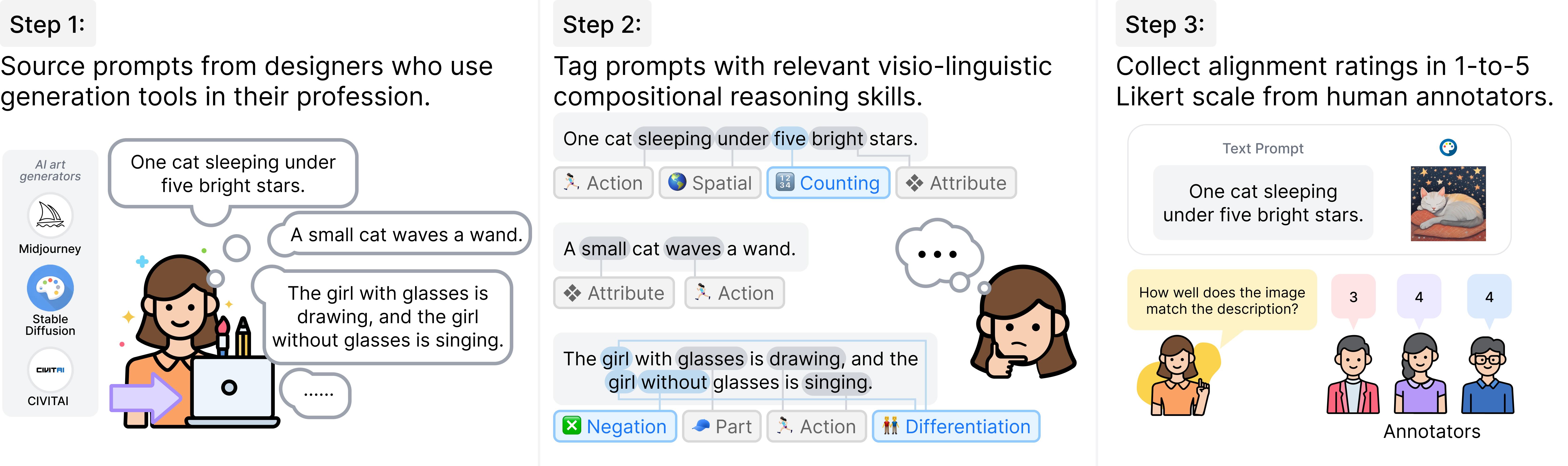

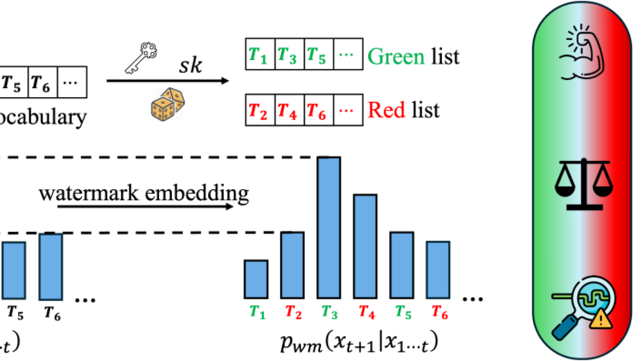


 Robustness. The goal of developing a watermark that is robust to output perturbations is to defend against watermark removal, which may be used to circumvent detection schemes for applications such as phishing or fake news generation. Robust watermark designs have been the topic of many recent works. A more robust watermark can better defend against watermark-removal attacks. However, our work shows that robustness can also enable piggyback spoofing attacks.
 Multiple Keys. Many works have explored the possibility of launching watermark stealing attacks to infer the secret pattern of the watermark, which can then boost the performance of spoofing and removal attacks. A natural and effective defense against watermark stealing is using multiple watermark keys during embedding, which can improve the unbiasedness property of the watermark (it is called distortion-free in the
  Public Detection API. It is still an open question whether watermark detection APIs should be made publicly available to users. Although this makes it easier to detect watermarked text, it is commonly acknowledged that it will make the system vulnerable to attacks. We study this statement more precisely by examining the specific risk trade-offs that exist, as well as introducing a novel defense that may make the public detection API more feasible in practice.