A series of regression instances in a pharmaceutical application. Can we learn how to set the regularization parameter (lambda) from similar domain-specific data?
Overview. Perhaps the simplest relation between a real dependent variable (y) and a vector of features (X) is a linear model (y = beta X). Given some training examples or datapoints consisting of pairs of features and dependent variables ((X_1, y_1),(X_2, y_2),dots,(X_m,y_m)), we would like to learn (beta) which would give the best prediction (y’) given features (X’) of an unseen example. This process of fitting a linear model (beta) to the datapoints is called linear regression. This simple yet effective model finds ubiquitous applications, ranging from biological, behavioral, and social sciences to environmental studies and financial forecasting, to make reliable predictions on future data. In ML terminology, linear regression is a supervised learning algorithm with low variance and good generalization properties. It is much less data-hungry than typical deep learning models, and performs well even with small amounts of training data. Further, to avoid overfitting the model to the training data, which reduces the prediction performance on unseen data, one typically uses regularization, which modifies the objective function of the linear model to reduce impact of outliers and irrelevant features (read on for details).
The most common method for linear regression is “regularized least squares”, where one finds the (beta) which minimizes
$$||y – beta X||_2^2 + lambda ||beta||.$$
Here the first term captures the error of (beta) on the training set, and the second term is a norm-based penalty to avoid overfitting (e.g. reducing impact of outliers in data). How to set (lambda) appropriately in this fundamental method depends on the data domain and is a longstanding open question. In typical modern applications, we have access to several similar datasets (X^{(0)},y^{(0)}, X^{(1)},y^{(1)}, dots) from the same application domain. For example, there are often multiple drug trial studies in a pharmaceutical company for studying the different effects of similar drugs. In this work, we show that we can indeed learn a good domain-specific value of (lambda) with strong theoretical guarantees of accuracy on unseen datasets from the same domain, and give bounds on how much data is needed to achieve this.
As our main result, we show that if the data has (p) features (i.e., the dimension of feature vector (X_i) is (p), then after seeing (O(p/epsilon^2)) datasets, we can learn a value of (lambda) which has error (averaged over the domain) within (epsilon) of the best possible value of (lambda) for the domain. We also extend our results to sequential data, binary classification (i.e. (y) is binary valued) and non-linear regression.
Problem Setup. Linear regression with norm-based regularization penalty is one of the most popular techniques that one encounters in introductory courses to statistics or machine learning. It is widely used for data analysis and feature selection, with numerous applications including medicine, quantitative finance (the linear factor model), climate science, and so on. The regularization penalty is typically a weighted additive term (or terms) of the norms of the learned linear model (beta), where the weight is carefully selected by a domain expert. Mathematically, a dataset has dependent variable (y) consisting of (m) examples, and predictor variables (X) with (p) features for each of the (m) datapoints. The linear regression approach (with squared loss) consists of solving a minimization problem
$$hat{beta}^{X,y}_{lambda_1,lambda_2}=text{argmin}_{betainmathbb{R}^p}||y-Xbeta||^2+lambda_1||beta||_1+lambda_2||beta||_2^2,$$
where the highlighted term is the regularization penalty. Here (lambda_1, lambda_2ge 0) are the regularization coefficients constraining the L1 and L2 norms, respectively, of the learned linear model (beta). For general (lambda_1) and (lambda_2) the above algorithm is popularly known as the Elastic Net, while setting (lambda_1 = 0) recovers Ridge regression and setting (lambda_2 = 0) corresponds to LASSO. Ridge and LASSO regression are both individually popular methods in practice, and the Elastic Net incorporates the advantages of both.
Despite the central role these coefficients play in linear regression, the problem of setting them in a principled way has been a challenging open problem for several decades. In practice, one typically uses “grid search” cross-validation, which involves (1) splitting the dataset into several subsets consisting of training and validation sets, (2) training several models (corresponding to different values of regularization coefficients) on each training set, and (3) comparing the performance of the models on the corresponding validation sets. This approach has several limitations.
- First, this is very computationally intensive, especially with the large datasets that typical modern applications involve, as one needs to train and evaluate the model for a large number of hyperparameter values and training-validation splits. We would like to avoid repeating this cumbersome process for similar applications.
- Second, theoretical guarantees on how well the coefficients learned by this procedure will perform on unseen examples are not known, even when the test data are drawn from the same distribution as the training set.
- Finally, this can only be done for a finite set of hyperparameter values and it is not clear how the selected parameter compares to the best parameter from the continuous domain of coefficients. In particular, the loss as a function of the regularization parameter is not known to be Lipschitz.
Our work addresses all three of the above limitations simultaneously in the data-driven setting, which we motivate and describe next.
The importance of regularization
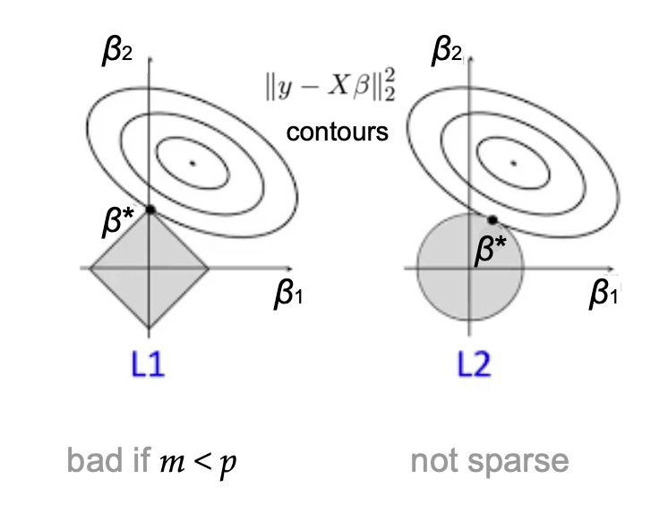
A visualization of the L1 and L2 regularized regressions.
The regularization coefficients (lambda_1) and (lambda_2) play a crucial role across fields: In machine learning, controlling the norm of model weights (beta) implies provable generalization guarantees and prevents over-fitting in practice. In statistical data analysis, their combined use yields parsimonious and interpretable models. In Bayesian statistics they correspond to imposing specific priors on (beta). Effectively, (lambda_2) regularizes (beta) by uniformly shrinking all coefficients, while (lambda_1) encourages the model vector to be sparse. This means that while they do yield learning-theoretic and statistical benefits, setting them to be too high will cause models to under-fit to the data. The question of how to set the regularization coefficients becomes even more unclear in the case of the Elastic Net, as one must juggle trade-offs between sparsity, feature correlation, and bias when setting both (lambda_1) and (lambda_2) simultaneously.
The data-driven algorithm design paradigm
In many applications, one has access to not just a single dataset, but a large number of similar datasets coming from the same domain. This is increasingly true in the age of big data, where an increasing number of fields are recording and storing data for the purpose of pattern analysis. For example, a drug company typically conducts a large number of trials for a variety of different drugs. Similarly, a climate scientist monitors several different environmental variables and continuously collects new data. In such a scenario, can we exploit the similarity of the datasets to avoid doing cumbersome cross-validation each time we see a new dataset? This motivates the data-driven algorithm design setting, introduced in the theory of computing community by Gupta and Roughgarden as a tool for design and analysis of algorithms that work well on typical datasets from an application domain (as opposed to worst-case analysis). This approach has been successfully applied to several combinatorial problems including clustering, mixed integer programming, automated mechanism design, and graph-based semi-supervised learning (Balcan, 2020). We show how to apply this analytical paradigm to tuning the regularization parameters in linear regression, extending the scope of its application beyond combinatorial problems [1, 2].
The learning model
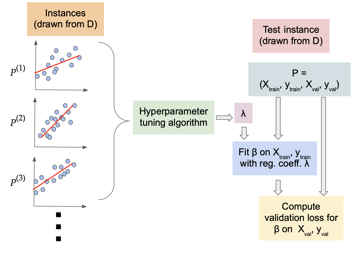
Formally, we model data coming from the same domain as a fixed (but unknown) distribution (D) over the problem instances. To capture the well-known cross-validation setting, we consider each problem instance of the form (P=(X_{text{train}}, y_{text{train}}, X_{text{val}}, y_{text{val}})). That is, the random process that generates the datasets and the (random or deterministic) process that generates the splits given the data, have been combined under (D). The goal of the learning process is to take (N) problem samples generated from the distribution (D), and learn regularization coefficients (hat{lambda}=(lambda_1, lambda_2)) that would generalize well over unseen problem instances drawn from (D). That is, on an unseen test instance (P’=(X’_{text{train}}, y’_{text{train}}, X’_{text{val}}, y’_{text{val}})), we will fit the model (beta) using the learning regularization coefficients (hat{lambda}) on (X’_{text{train}}, y’_{text{train}}), and evaluate the loss on the set (X’_{text{val}}, y’_{text{val}}). We seek the value of (hat{lambda}) that minimizes this loss, in expectation over the draw of the random test sample from (D).
How much data do we need?
The model (beta) clearly depends on both the dataset ((X,y)), and the regularization coefficients (lambda_1, lambda_2). A key tool in data-driven algorithm design is the analysis of the “dual function”, which is the loss expressed as a function of the parameters, for a fixed problem instance. This is typically easier to analyze than the “primal function” (loss for a fixed parameter, as problem instances are varied) in data-driven algorithm design problems. For Elastic Net regression, the dual is the validation loss on a fixed validation set for models trained with different values of (lambda_1, lambda_2) (i.e. two-parameter function) for a fixed training set. Typically the dual functions in combinatorial problems exhibit a piecewise structure, where the behavior of the loss function can have sharp transitions across the pieces. For example, in clustering this piecewise behavior could correspond to learning a different cluster in each piece. Prior research has shown that if we can bound the complexity of the boundary and piece functions in the dual function, then we can give a sample complexity guarantee, i.e. we can answer the question “how much data is sufficient to learn a good value of the parameter?”
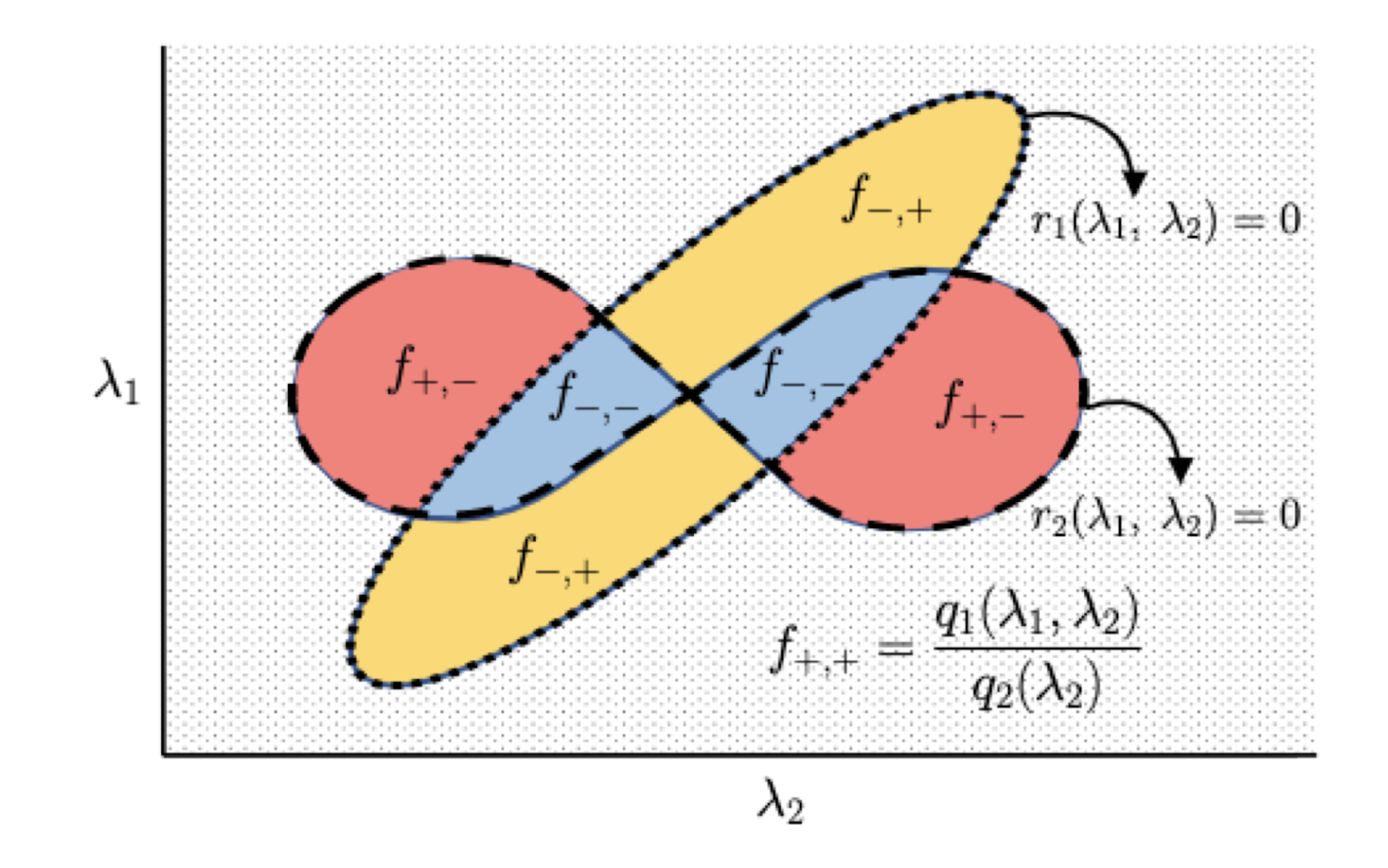
An illustration of the piecewise structure of the Elastic Net dual loss function. Here (r_1) and (r_2) are polynomial boundary functions, and (f_{*,*}) are piece functions which are fixed rational functions given the signs of boundary functions.
Somewhat surprisingly, we show that the dual loss function exhibits a piecewise structure even in linear regression, a classic continuous optimization problem. Intuitively, the pieces correspond to different subsets of the features being “active”, i.e. having non-zero coefficients in the learned model (beta). Specifically, we show that the piece boundaries of the dual function are polynomial functions of bounded degree, and the loss within each piece is a rational function (ratio of two polynomial functions) again of bounded degree. We use this structure to establish a bound on the learning-theoretic complexity of the dual function; more precisely, we bound its pseudo-dimension (a generalization of the VC dimension to real-valued functions).
Theorem. The pseudo-dimension of the Elastic Net dual loss function is (Theta(p)), where (p) is the feature dimension.
(Theta(p)) notation here means we have an upper bound of (O(p)) as well as a lower bound (Omega(p)) on the pseudo-dimension. Roughly speaking, the pseudo-dimension captures the complexity of the function class from a learning perspective, and corresponds to the number of samples needed to guarantee small generalization error (average error on test data). Remarkably, we show an asymptotically tight bound on the pseudo-dimension by establishing a (Omega(p)) lower bound which is technically challenging and needs an explicit construction of a collection of “hard” instances. Tight lower bounds are not known for several typical problems in data-driven algorithm design. Our bound depends only on (p) (the number of features) and is independent of the number of datapoints (m). An immediate consequence of our bound is the following sample complexity guarantee:
Theorem. Given any distribution (D) (fixed, but unknown), we can learn regularization parameters (hat{lambda}) which obtain error within any (epsilon>0) of the best possible parameter with probability (1-delta) using only (O(1/epsilon^2(p+log 1/delta))) problem samples.
One way to understand our results is to instantiate them in the cross-validation setting. Consider the commonly used techniques of leave-one-out cross validation (LOOCV) and Monte Carlo cross validation (repeated random test-validation splits, typically independent and in a fixed proportion). Given a dataset of size (m_{text{tr}}), LOOCV would require (m_{text{tr}}) regression fits which can be computationally expensive for large datasets. Alternately, we can consider draws from a distribution (D_{text{LOO}}) which generates problem instances P from a fixed dataset ((X, y) in R^{m+1times p} times R^{m+1}) by uniformly selecting (j in [m + 1]) and setting (P = (X_{−j∗}, y_{−j} , X_{j∗}, y_j )). Our result now implies that roughly (O(p/epsilon^2)) iterations are enough to determine an Elastic Net parameter (hat{lambda}) with loss within (epsilon) (with high probability) of the parameter (lambda^*) obtained from running the full LOOCV. Similarly, we can define a distribution (D_{text{MC}}) to capture the Monte Carlo cross validation procedure and determine the number of iterations sufficient to get an (epsilon)-approximation of the loss corresponding parameter selection with an arbitrarily large number of runs. Thus, in a very precise sense, our results answer the question of how much cross-validation is enough to effectively implement the above techniques.
Sequential data and online learning
A more challenging variant of the problem assumes that the problem instances arrive sequentially, and we need to set the parameter for each instance using only the previously seen instances. We can think of this as a game between an online adversary and the learner, where the adversary wants to make the sequence of problems as hard as possible. Note that we no longer assume that the problem instances are drawn from a fixed distribution, and this setting allows problem instances to depend on previously seen instances which is typically more realistic (even if there is no actual adversary generating worst-case problem sequences). The learner’s goal is to perform as well as the best fixed parameter in hindsight, and the difference is called the “regret” of the learner.
To obtain positive results, we make a mild assumption on the smoothness of the data: we assume that the prediction values (y) are drawn from a bounded density distribution. This captures a common data pre-processing step of adding a small amount of uniform noise to the data for model stability, e.g. by setting the jitter parameter in the popular Python library scikit-learn. Under this assumption, we show further structure on the dual loss function. Roughly speaking, we show that the location of the piece boundaries of the dual function across the problem instances do not concentrate in a small region of the parameter space.This in turn implies (using Balcan et al., 2018) the existence of an online learner with average expected regret (O(1/sqrt{T})), meaning that we converge to the performance of the best fixed parameter in hindsight as the number of online rounds (T) increases.
Extension to binary classification, including logistic regression
Linear classifiers are also popular for the task of binary classification, where the (y) values are now restricted to (0) or (1). Regularization is also crucial here to learn effective models by avoiding overfitting and selecting important variables. It is particularly common to use logistic regression, where the squared loss above is replaced by the logistic loss function,
$$l_{text{RLR}}(beta,(X,y))=frac{1}{m}sum_{i=1}^mlog(1+exp(-y_ix_i^Tbeta)).$$
The exact loss minimization problem is significantly more challenging in this case, and it is correspondingly difficult to analyze the dual loss function. We overcome this challenge by using a proxy dual function which approximates the true loss function, but has a simpler piecewise structure. Roughly speaking, the proxy function considers a fine parameter grid of width (epsilon) and approximates the loss function at each point on the grid. Furthermore, it is piecewise linear and known to approximate the true loss function to within an error of (O(epsilon^2)) at all points (Rosset, 2004).
Our main result for logistic regression is that the generalization error with (N) samples drawn from the distribution (D) is bounded by (O(sqrt{(m^2+log 1/epsilon)/N}+epsilon^2+sqrt{(log 1/delta)/N})), with (high) probability (1-delta) over the draw of samples. (m) here is the size of the validation set, which is often small or even constant. While this bound is incomparable to the pseudo-dimension-based bounds above, we do not have lower bounds in this setting and tightness of our results in an interesting open question.
Beyond the linear case: kernel regression
So far, we have assumed that the dependent variable (y) has a linear dependence on the predictor variables. While this is a great first thing to try in many applications, very often there is a non-linear relationship between the variables. As a result, linear regression can result in poor performance in some applications. A common alternative is to use Kernelized Least Squares Regression, where the input (X) is implicitly mapped to high (or even infinite) dimensional feature space using the “kernel trick”. As a corollary of our main results, we can show that the pseudo-dimension of the dual loss function in this case is (O(m)), where (m) is the size of the training set in a single problem instance. Our results do not make any assumptions on the (m) samples within a problem instance/dataset; if these samples within problem instances are further assumed to be i.i.d. draws from some data distribution (distinct from problem distribution (D)), then well-known results imply that (m = O(k log p)) samples are sufficient to learn the optimal LASSO coefficient ((k) denotes the number of non-zero coefficients in the optimal regression fit).
Some final remarks
We consider how to tune the norm-based regularization parameters in linear regression. We pin down the learning-theoretic complexity of the loss function, which may be of independent interest. Our results extend to online learning, linear classification, and kernel regression. A key direction for future research is developing an efficient implementation of the algorithms underlying our approach.
More broadly, regularization is a fundamental technique in machine learning, including deep learning where it can take the form of dropout rates, or parameters in the loss function, with significant impact on the performance of the overall algorithm. Our research opens up the exciting question of tuning learnable parameters even in continuous optimization problems. Finally, our research captures an increasingly typical scenario with the advent of the data era, where one has access to repeated instances of data from the same application domain.
For further details about our cool results and the mathematical machinery we used to derive them, check out our papers linked below!
[1] Balcan, M.-F., Khodak, M., Sharma, D., & Talwalkar, A. (2022). Provably tuning the ElasticNet across instances. Advances in Neural Information Processing Systems, 35. [2] Balcan, M.-F., Nguyen, A., & Sharma, D. (2023). New Bounds for Hyperparameter Tuning of Regression Problems Across Instances. Advances in Neural Information Processing Systems, 36.