Introducing hierarchical deletion to easily clean up unused resources in Amazon Forecast

Amazon Forecast just launched the ability to hierarchically delete resources at a parent level without having to locate the child resources. You can stay focused on building value-adding forecasting systems and not worry about trying to manage individual resources that are created in your workflow. Forecast uses machine learning (ML) to generate more accurate demand forecasts, without requiring any prior ML experience. Forecast brings the same technology used at Amazon.com to developers as a fully managed service, removing the need to manage resources or rebuild your systems.

When importing data, training a predictor, and creating forecasts, Forecast generates resources related to the dataset group. For example, when a predictor is generated using a dataset group, the predictor is the child resource and the dataset group is the parent resource. Previously, it was difficult to delete resources while building your forecasting system because you had to delete the child resources first, and then delete the parent resources. This was especially difficult and time-consuming because deleting resources required you to understand the various resource hierarchies, which weren’t immediately visible.

As you experiment and create multiple dataset groups, predictors, and forecasts, the resource hierarchy can become complicated. However, this streamlined hierarchical deletion method allows you to quickly clean up resources without having to worry about understanding the resource hierarchy.

In this post, we walk through the Forecast console experience of deleting all the resource types that are supported by Forecast. You can also perform hierarchical deletion by referencing the Deleting Resources page. To delete individual or child resources one at a time, you can continue to use the existing APIs such as DeleteDataset, DeleteDatasetGroup, DeleteDatasetImportJob, DeleteForecast, DeleteForecastExportJob, DeletePredictor and DeletePredictorBacktestExportJob.

Delete dataset group resources

To delete a dataset group when it doesn’t have any child resources, a simple dialog is displayed. You can delete the chosen resource by entering delete and choosing Delete.

When a dataset group has underlying child resources such as predictors, predictor backtest export jobs, forecasts, and forecast export jobs, a different dialog is displayed. After you enter delete and choose Delete, all these child resources are deleted, including the selected dataset group resource.

Delete dataset resources

For a dataset resource without child resources, you see a simple dialog is during the delete operation.

When a dataset has child dataset import jobs, the following dialog is displayed.

Delete predictor resources

For a predictor resource without child resources, the following simple dialog is displayed.

When the predictor resource has underlying child resources such as predictor backtest export jobs, forecasts, or forecast export jobs, the following dialog is displayed. If you proceed with the delete action, all these child resources are deleted, including the selected predictor resource.

Delete a forecast resource

For a forecast resource without child resources, the following dialog is displayed.

When a forecast resource has underlying child resources such as forecast export jobs, the following dialog is displayed.

Delete dataset import job, predictor backtest export job, or forecast export job resources

The dataset import job, predictor backtest export job, and forecast export job resources don’t have any child resources. Therefore, when you choose to delete any of these resources via the Forecast console, a simple delete dialog is displayed. When you proceed with the delete, only the selected resources are deleted.

For example, when deleting a dataset import job resource, the following dialog is displayed.

Conclusion

You now have more flexibility when deleting a resource or an entire hierarchy of resources. To get started with this capability, see the Deleting Resources page and go through the notebook in our GitHub repo that walks you through how to perform hierarchical deletion. You can use this capability in all Regions where Forecast is publicly available. For more information about Region availability, see AWS Regional Services.


About the Authors

Alex Kim is a Sr. Product Manager for Amazon Forecast. His mission is to deliver AI/ML solutions to all customers who can benefit from it. In his free time, he enjoys all types of sports and discovering new places to eat.


Ranga Reddy Pallelra works as an SDE on the Amazon Forecast team. In his current role, he works on large-scale distributed systems with a focus on AI/ML. In his free time, he enjoys listening to music, watching movies, and playing racquetball.


Shannon Killingsworth is a UX Designer for Amazon Forecast and Amazon Personalize. His current work is creating console experiences that are usable by anyone, and integrating new features into the console experience. In his spare time, he is a fitness and automobile enthusiast.

Read More

PLAS: Latent Action Space for Offline Reinforcement Learning

Figure 1: Overview: To avoid out-of-distribution actions in the Offline Reinforcement Learning problem, we propose to implicitly constrain the policy by modifying the action space instead of enforcing explicit constraints. The policy is trained to output a latent action which will be passed into a decoder pretrained with the dataset. We demonstrate that our method provides competitive performance in both simulation and real-robot experiments.

Offline RL: Learning a policy from a static dataset

The goal of Reinforcement Learning (RL) is to learn to perform a task by interacting with the environment. It has achieved significant success in a lot of applications such as games and robotics. One major challenge in RL is that it requires a huge amount of interactive data collected in the environment to learn a policy. However, data collection is expensive and potentially dangerous in many real-world applications, such as robotics in safety-critical situations (e.g., around humans) or healthcare problems. Worse, RL algorithms also usually assume that the dataset used to update the policy comes from the current policy or its own training process.

To use data more wisely, we may consider Offline Reinforcement Learning. The goal of offline RL is to learn a policy from a static dataset of transitions without further data collection. Although we may still need a large amount of data, the assumption of static datasets allows more flexibility in data collection. For example, in robotics, we can include human demonstrations, reuse rollouts from previous experiments, and share data within the community. In this way, the dataset is more likely to be scaled up in size even when data collection is expensive.

Figure 2: In contrast to a common reinforcement learning pipeline that collects data and updates the policy alternatively, Offline Reinforcement Learning aims to learn a policy from a static dataset without further data collection.

One important feature of offline RL is that it requires no assumption about the performance of the policy that is used to collect the dataset. This is in contrast to behavior cloning, where we assume that the dataset is collected by an expert, so that we can directly “copy” the actions given states without reasoning about the future reward. In offline RL, the dataset could be collected by a policy (or several policies) with arbitrary performance.

At first glance, off-policy algorithms seem to be able to meet the above requirements. Off-policy algorithms save the agent’s interactions during training in a replay buffer and train the policy by sampling transitions from the replay buffer (Lillicrap 2015, Haarnoja 2018). However, as shown in previous work (Fujimoto 2018b), when we apply off-policy algorithms to a static dataset, the performance can be very poor due to out-of-distribution actions. In the off-policy algorithm, the Q-function is updated by the Bellman operator:

$$ mathcal{T} hat{Q}^pi(s_t, a_t) = mathbb{E}_{r_t, s_{t+1}}[r_t + gamma hat{Q}^pi(s_{t+1}, pi(s_{t+1}))] $$

As explained in Fujimoto (2018b), if the policy selects an action (pi(s_{t+1})) that is not included in this static dataset, then the term (hat{Q}^pi(s_{t+1},pi(s_{t+1}))) may have a large extrapolation error. The extrapolation error will be accumulated by the Bellman operator and exacerbated by the policy updates. These errors eventually lead to significant overestimation bias that can hurt the performance. This has always been an issue for Q-learning-based methods (Thrun 1993, Fujimoto 2018a), but it is especially problematic when applied on a static dataset because the policy is not able to try out and correct the overly-optimistic actions. The problem is more significant when the action space is large, such as continuous action space with high dimensions.

Objectives for Offline RL algorithms to avoid out-of-distribution actions

To fix the issue discussed above and to fully utilize the dataset, we need two objectives in offline RL. First, the policy should be constrained to select actions within the support of the dataset. The policy that represents the probability distribution (p(a|s)) of the dataset is usually called the behavior policy, denoted as (pi_B). We aim to maximize the return of the policy (G_t) subject to the constraint that (pi_B(a|s)) is larger than a threshold (epsilon):

$$ max_{asim pi(cdot|s)} mathbb{E}[G_t]$$
$$ s.t. pi_B(a|s) > epsilon$$

An illustration of this constraint is shown in Figure 3 below. Given a behavior policy ( pi_B(a|s) ) on the top figure, the agent policy ( pi) should only choose actions within the green region where ( pi_B(a|s) > epsilon). On the other hand, the constraint cannot be overly restrictive.  Specifically, the policy should not be affected by the density of (pi_B). In the example in Figure 3, the policy should have the flexibility to choose any action within the green region even if it deviates from the most probable action of (pi_B) and the “shape” of the distribution (pi) is very different from the shape of (pi_B).

Figure 3: An illustration of the two objectives of offline RL: Given a behavior policy distribution at a state (s) (top), the policy (bottom) should (1) only choose actions within the green region where (pi_B > epsilon) (2) not be restricted by the density of the behavior policy (pi_B).

Figure 4 below shows a more intuitive example. Consider an agent in a grid world. Suppose that the agent has a dataset of transitions marked as blue dots and arrows. The agent aims to find a path to get to the goal without the information of the other parts of the map. As shown on the left figure, it cannot select out-of-distribution actions because it might be dangerous. As shown on the right figure, if action (a_1) appears 10 times in the dataset, and action (a_0) appears 5 times in the dataset, it should not choose action (a_1) just because it appears more often in the dataset; as shown, this might be a suboptimal action for the task.

Figure 4: An intuitive explanation of the two objectives in offline RL: (1) Left: Choosing out-of-distribution actions may lead to a dangerous state. (2) Right: The action selection given a state should not be biased by the probability of the actions of the dataset.

Previous methods struggled with achieving both of these objectives. For example, BCQ (Fujimoto 2018b) proposes to sample from the behavior policy, perturb around it and then take the action that maximizes the Q-value. This method will be restricted by the density of the behavior policy distribution if the sample size 𝑁 is not large enough. Another line of work uses explicit policy constraints in the optimization process (Jaques 2019, Kumar 2019, Wu 2019). They try to force the agent policy to be close to the behavior policy in terms of different measures of distance, such as KL or MMD (Figure 1). The explicit constraints create difficulties in the optimization and distance metrics such as KL will be affected by the density (see Appendix E in our paper). 

Proposed Method: Policy in Latent Action Space (PLAS)

In our paper, PLAS: Latent Action Space for Offline Reinforcement Learning (CoRL 2020), we propose a method that can satisfy both the objectives discussed above by simply modifying the action space of the policy – i.e., the policy will only select actions when ( pi_B(a|s) > epsilon), but will not be restricted by the density of the distribution ( pi_B(a|s)). In our method, we first model the behavior policy using a Conditional Variational Autoencoder (CVAE) as in previous work (Fujimoto 2018b, Kumar 2019). The CVAE is trained to reconstruct actions conditioned on the states. The decoder of the CVAE creates a mapping from the latent space to the action space. Instead of training a policy in the action space of the environment, we propose to learn a Policy in the Latent Action Space (PLAS) of the CVAE and then use the pretrained decoder to output an action in the original action space.

Figure 5: Proposed Method: Policy in Latent Action Space (PLAS). We propose to first train a CVAE using the dataset and freeze the decoder. Second, we train a policy in the latent action space. The latent action will be passed into the decoder and transformed into an action within the distribution of the dataset. In contrast to previous work, it forms an implicit policy constraint in the latent action space.

Using the above approach, we can naturally constrain the policy to select actions within the dataset because the action is chosen from the latent space. The prior of the latent variable of CVAE is set to be a normal distribution for simplicity, following the common practice. To constrain the latent policy from selecting actions that are too “far away” from this prior, we use a tanH activation at the output of the policy; this implicitly constrains the policy to select within a fixed number of standard deviations of the mean of the latent prior. It is important to note that the action output from the decoder should be conditioned on the state because we care about (pi_B(a|s) > epsilon) instead of (pi_B(a)>epsilon). This approach also satisfies the second objective because the policy can select any action within the latent space and will not be affected by the density of the behavior policy. 

Experiments: Cloth Sliding and D4RL benchmark

This modification over the action space can be built on top of any off-policy algorithm with either a stochastic or deterministic policy. In our experiment, we use TD3 (Fujimoto 2018a) with a deterministic latent policy. We evaluate our algorithm on a wide range of continuous control tasks, including a real robot experiment on cloth sliding and the D4RL benchmark

The task for the real-robot experiment is to slide along the edge of the cloth without dropping it. The dataset we use consists of a replay buffer from a previous experiment (around 7000 timesteps) and 5 episodes of expert trajectories (around 300 timesteps). Our method outperforms all the baselines and achieves similar performance as the expert.

Figure 6: Results from the real robot experiment. Left: Performance of PLAS on the cloth-sliding task. More videos can be found here. Right: Training curves of PLAS and the baselines. PLAS outperforms the other baselines and achieves similar performance as the expert. 

On the D4RL benchmark, our method also achieves consistent performance across a wide range of datasets with different environments and qualities despite its simplicity. We provide some of the qualitative and quantitative results below in Figures 7 and 8. Check out the full results on the D4RL benchmark in the paper. More videos can be found on our website.

Figure 7: We evaluate our method on different environments and datasets from the D4RL benchmark. Here are some examples of trained policies in Hopper-v2, Walker2d-v2, Adroit Hammer, and the FrankaKitchen environment. The policies are able to perform the tasks without further data collection. More videos can be found here.
Figure 8: Training curves on the medium expert datasets on the locomotion tasks. Our method achieves comparable performance as the expert on the medium expert datasets. More results can be found in the paper.

To further analyze the result, we plot the estimation error of the learned Q-functions in Figure 9. During the evaluation, we compare the estimated Q-value of the state-action pairs with their true return from the rollouts. Our method has the lowest mean squared error (MSE) while the baselines have either more significant overestimation or underestimation.

Figure 9: Analysis of Q-functions on the Walker2d-v2 Medium Expert dataset: (a) Mean squared error (b) The percentage of overestimated Q-values. Our method has the lowest MSE without significant overestimation or underestimation.

As mentioned earlier in the objectives, our method focuses on avoiding out-of-distribution actions. In our experiment, we analyze the effect of out-of-distribution actions by introducing an additional component: we add a perturbation layer that is trained together with the latent policy, inspired by Fujimoto 2018b. The perturbation layer outputs a residual over the action output of the decoder. This allows the final policy output to deviate from the support of the dataset in a controlled way. More precisely, restricting the range of the output of the perturbation layer is essentially constraining the action output to be close to the dataset in terms of the L-infinity norm. In Figure 10, we plot the performance of our method with different ranges of allowed perturbation. We found that out-of-distribution actions introduced by the perturbation layer are usually harmful to datasets with high-quality rollouts such as the medium-expert datasets. However, it could be helpful for some of the random or medium datasets depending on the environment. The full analysis of the perturbation layer can be found in Appendix D. The results shed light on the disentangled contributions of in-distribution generalization and out-of-distribution generalization in offline reinforcement learning.

Figure 10: Effect of the perturbation layer on different datasets. More allowed perturbation is usually harmful to the datasets with high-quality rollouts such as the medium expert datasets, but it could be helpful for the medium or random datasets for certain environments.

Conclusion and Discussion

We propose a simple and straightforward approach to offline RL: Policy in the Latent Action Space (PLAS). To summarize:

  • Our approach naturally avoids out-of-distribution actions while allowing the flexibility for improvement over the performance of the dataset through implicit constraints.
  • It achieves competitive performance in both simulated environments and a real robot experiment on cloth manipulation.
  • We provided the analyses on Q-function estimation error and the separation of in-distribution vs. out-of-distribution generalization in Offline RL.

Please visit our website for the paper, code, and more videos.

Our method can be extended in different ways. First, it will benefit from a better generative model. For example, using normalizing flow to replace VAE could potentially lead to theoretical guarantees and better evaluation performance. Second, it can also be extended to allow better “out-of-distribution” generalization. We hope that our method will pave the way for future possibilities of applying reinforcement learning algorithms to real-world applications by using the static datasets more efficiently.

Acknowledgements

This material is based upon work supported by the United States Air Force and DARPA under Contract No. FA8750-18-C-0092, LG Electronics and the National Science Foundation under Grant No. IIS-1849154. Any opinions, findings, and conclusions or recommendations expressed in this material are those of the author(s) and do not necessarily reflect the views of United States Air Force and DARPA and the National Science Foundation.

DISCLAIMER: All opinions expressed in this post are those of the author and do not represent the views of Carnegie Mellon University.

Read More

Around the World in AI Ways: Video Explores Machine Learning’s Global Impact

You may have used AI in your smartphone or smart speaker, but have you seen how it comes alive in an artist’s brush stroke, how it animates artificial limbs or assists astronauts in Earth’s orbit?

The latest video in the “I Am AI” series — the annual scene setter for the keynote at NVIDIA’s GTC — invites viewers on a journey through more than a dozen ways this new and powerful form of computing is expanding horizons.

Perhaps your smart speaker woke you up this morning to music from a distant radio station. Maybe you used AI in your smartphone to translate a foreign phrase in a book you’re reading.

A View of What’s to Come

These everyday use cases are becoming almost commonplace. Meanwhile, the frontiers of AI are extending to advance more critical needs.

In healthcare, the Bionic Vision Lab at UC Santa Barbara uses deep learning and virtual prototyping on NVIDIA GPUs to develop models of artificial eyes. They let researchers explore the potential and limits of a design for artificial eyes by viewing a model through a virtual-reality headset.

At Canada’s University of Waterloo, researchers are using AI to develop autonomous controls for exoskeleton legs that help users walk, climb stairs and avoid obstacles. Wearable cameras filter video through AI models trained on NVIDIA GPUs to recognize surrounding features such as stairs and doorways and then determine the best movements to take.

“Similar to autonomous cars that drive themselves, we’re designing autonomous exoskeletons that walk for themselves,” Brokoslaw Laschowski, a lead researcher on the ExoNet project, said in a recent blog.

Watch New Worlds Come to Life

In “I Am AI,” we meet Sofia Crespo who calls herself a generative artist. She blends and morphs images of jellyfish, corals and insects in videos that celebrate the diversity of life, using an emerging form of AI called generative adversarial networks and neural network models like GPT-2.

Sofia Crespo uses GANs
A fanciful creature created by artist Sofia Crespo using GANs.

“Can we use these technologies to dream up new biodiversities that don’t exist? What would these creatures look like?” she asks in a separate video describing her work.

See How AI Guards Ocean Life

“I Am AI” travels to Hawaii, Morocco, the Seychelles and the U.K., where machine learning is on the job protecting marine life from very real threats.

In Africa, the ATLAN Space project uses a fleet of autonomous drones with AI-powered computer vision to detect illegal fishing and ships dumping oil into the sea.

On the other side of the planet, the Maui dolphin is on the brink of extinction, with only 63 adults in the latest count. A nonprofit called MAUI63 uses AI in drones to identify individuals by their fin markings, tracking their movements so policy makers can take steps such as creating marine sanctuaries to protect them.

Taking the Planet’s Temperature

AI is also at work developing the big picture in planet ecology.

The video spotlights the Plymouth Marine Laboratory in the UK, where researchers use an NVIDIA DGX system to analyze data gathered on the state of our oceans. Their work contributes to the U.N. Sustainable Development Goals and other efforts to monitor the health of the seas.

A team of Stanford researchers is using AI to track wildfire risks. The video provides a snapshot of their work opening doors to deeper understandings of how ecosystems are affected by changes in water availability and climate.

Beam Me Up, NASA

The sky’s the limit with the Spaceborne Computer-2, a supercharged system made by Hewlett Packard Enterprise now installed in the International Space Station. It packs NVIDIA GPUs that astronauts use to monitor their health in real time and track objects in space and on Earth like a cosmic traffic copter.

The ISS now packs an NVIDIA GPU.
Astronauts use Spaceborne Computer-2 to run AI experiments on the ISS.

One of the coolest things about Spaceborne Computer-2 is you can suggest an experiment to run on it. HPE and NASA extended an open invitation for proposals, so Earth-bound scientists can expand the use of AI in space.

If these examples don’t blow the roof off your image of where machine learning might go next, check out the full “I Am AI” video below. It includes several more examples of other AI projects in art, science and beyond.

The post Around the World in AI Ways: Video Explores Machine Learning’s Global Impact appeared first on The Official NVIDIA Blog.

Read More

Translate All: Automating multiple file type batch translation with AWS CloudFormation

This is a guest post by Cyrus Wong, an AWS Machine Learning Hero. You can learn more about and connect with AWS Machine Learning Heroes at the community page

On July 29, 2020, AWS announced that Amazon Translate now supports Microsoft Office documents, including .docx, .xlsx, and .pptx.

The world is full of bilingual countries and cities like Hong Kong. I find myself always needing to prepare Office documents and presentation slides in both English and Chinese. Previously, it could be quite time-consuming to prepare the translated documents manually, and this approach can also lead to more errors. If I try to just select all, copy, and paste into a translation tool, then copy and paste the result into a new file, I lose all the formatting and images! My old method was to copy content piece by piece, translate it, then copy and paste it into the original document, over and over again. The new support for Office documents in Amazon Translate is really great news for teachers like me. It saves you a lot of time!

Still, we have to sort the documents by their file types and call Amazon Translate separately for different file types. For example, if I have notes in .docx files, presentations in .pptx files, and data in .xlsx files, I still have to sort them by their file type and send different TextTranslation API calls. In this post, I show how to sort content by document type and make batch translation calls. This solution automates the undifferentiated task of sorting files.

For my workflow, I need to upload all my course materials in a single Amazon Simple Storage Service (Amazon S3) bucket. This bucket often includes different types of files in one folder and subfolders.

However, when I start the Amazon Translate job on the console, I have to choose the file content type. The problem arises when different file types are in one folder without subfolders.

Therefore, our team developed a solution that we’ve called Translate All—a simple AWS serverless application to resolve those challenges and make it easier to integrate with other projects. A serverless architecture is a way to build and run applications and services without having to manage infrastructure. Your application still runs on servers, but all the server management is done by AWS. You no longer have to provision, scale, and maintain servers to run your applications, databases, and storage systems. For more information about serverless computing, see Serverless on AWS.

Solution overview

We use the following AWS services to run this solution:

  • AWS Lambda – This serverless compute service lets you run code without provisioning or managing servers, creating workload-aware cluster scaling logic, maintaining event integrations, or managing runtimes. With Lambda, you can run code for virtually any type of application or backend service—all with zero administration.
  • Amazon Simple Notification Service – Amazon SNS is a fully managed messaging service for both application-to-application (A2A) and application-to-person (A2P) communication. The A2A pub/sub functionality provides topics for high-throughput, push-based, many-to-many messaging between distributed systems, microservices, and event-driven serverless applications.
  • Amazon Simple Queue Service – Amazon SQS is a fully managed message queuing service that enables you to decouple and scale microservices, distributed systems, and serverless applications. Amazon SQS eliminates the complexity and overhead associated with managing and operating message-oriented middleware, and empowers developers to focus on differentiating work.
  • AWS Step Functions – This serverless function orchestrator makes it easy to sequence Lambda functions and multiple AWS services into business-critical applications. Through its visual interface, you can create and run a series of checkpointed and event-driven workflows that maintain the application state. The output of one step acts as an input to the next. Each step in your application runs in order, as defined by your business logic.

In our solution, if a JSON message is sent to the SQS queue, it triggers a Lambda function to start a Step Functions state machine (see the following diagram).

The state machine includes the following high-level steps:

  1. In the Copy to Type Folder stage, the state machine gets all the keys under InputS3Uri and copies each type of file into a type-specific, individual folder. If subfolders exist, it replaces / with _ForwardSlash_.

The following screenshot shows the code for this step.

The following screenshot shows the output files.

  1. The Parallel Map stage arranges the data according to contentTypes and starts the translation job workflow in parallel.

  1. The Start Translation Job workflow loops for completion status until all translate jobs are complete.
  2. In the Copy to Parent Folder stage, the step machine reconstructs the original input folder structure and generates a signed URL that remains valid for 7 days.
  3. The final stage publishes the results to Amazon SNS.

Additional considerations

When implementing this solution, consider the following:

  • As of this writing, we just handle the happy path and assume that all jobs are in Completed status at the end
  • The default job completion maximum period is 180 minutes; you can change the NumberOfIteration variable to extend it as needed
  • You can’t use the reserved words for file name or folder name: !!plain!!, !!html!!, !!document!!, !!presentation!!, !!sheet!!, !!document!!, or -_ForwardSlash_-

Deploy the solution

To deploy this solution, complete the following steps:

  1. Open the Serverless Application Repository link.
  2. Select I acknowledge that this app creates custom IAM roles.
  3. Choose Deploy.

  1. When the AWS CloudFormation console appears, note the input and output parameters on the Outputs

Test the solution

In this section, we walk you through using the application.

  1. On the Amazon SQS console, subscribe your email to TranslateCompletionSNSTopic .
  2. Upload all files into the folder InputBucket.
  3. Send a message to TranlateQueue. See the following example code:
{
  "JobName": "testing",
  "InputBucket": "//enter your InputBucket from the CloudFormation console//",
  "InputS3Uri": "test",
  "OutputBucket": "//enter your OutputBucket from the CloudFormation console//",
  "SourceLanguageCode": "en",
  "TargetLanguageCodes": [
    "zh-TW"
  ]
}

You receive the translation job result as an email.

The email contains a presigned URL with 7-day valid period. You can share the translated file without having to sign in to the AWS Management Console.

Conclusion

With this solution, my colleagues and I easily resolved our course materials translation problem. We saved a lot of time compared to opening the files one by one and copy-and-pasting repeatedly. The translation quality is good and eliminates the potential for errors that can often come with undifferentiated manual workflows. Now we can just use the AWS Command Line Interface (AWS CLI) to run the Amazon S3 sync command to upload our files into an S3 bucket and translate the all the course materials at once. Using this tool to leverage a suite of powerful AWS services has empowered my team to spend less time processing course materials and more time educating the next generation of cloud technology professionals!

Project collaborators include Mike Ng, Technical Program Intern at AWS, Brian Cheung, Sam Lam, and Pearly Law from the IT114115 Higher Diploma in Cloud and Data Centre Administration. This post was edited with Greg Rushing’s contribution.


The content and opinions in this post are those of the third-party author and AWS is not responsible for the content or accuracy of this post.


About the Author

Cyrus Wong is Data Scientist of Cloud Innovation Centre at the IT Department of the Hong Kong Institute of Vocational Education (Lee Wai Lee). He has achieved all 13 AWS Certifications and actively promotes the use of AWS in different media and events. His projects received four Hong Kong ICT Awards in 2014, 2015, and 2016, and all winning projects are running solely on AWS with Data Science and Machine Learning.

Read More

Flexible, Scalable, Differentiable Simulation of Recommender Systems with RecSim NG

Posted by Martin Mladenov, Research Scientist and Chih-wei Hsu, Software Engineer, Google Research

Recommender systems are the primary interface connecting users to a wide variety of online content, and therefore must overcome a number of challenges across the user population in order to serve them equitably. To this end, in 2019 we released RecSim, a configurable platform for authoring simulation environments to facilitate the study of RL algorithms (the de facto standard ML approach for addressing sequential decision problems) in recommender systems. However, as the technology has progressed, it has become increasingly important to address the gap between simulation and real-world applications, ensuring that models are flexible and easily extendible, enabling probabilistic inference of user dynamics, and addressing computational efficiency.

To address these issues, we recently released RecSim NG, the “Next Generation” of simulators for recommender systems research and development. RecSim NG is a response to a set of use cases that have emerged as important challenges in the application of simulation to real-world problems. It addresses the gap between simulation and real-world applications, ensures the models are flexible and easily extendible, enables probabilistic inference of user dynamics, and addresses computational efficiency.

Overview of RecSim NG
RecSim NG is a scalable, modular, differentiable simulator implemented in Edward2 and TensorFlow. It offers a powerful, general probabilistic programming language for agent-behavior specification.

RecSim NG significantly expands the modeling capabilities of RecSim in two ways. First, the story API allows the simulation of scenarios where an arbitrary number of actors (e.g., recommenders, content consumers, content producers, advertisers) interact with one another. This enables the flexible modeling of entire recommender ecosystems, as opposed to the usual isolated user-recommender interaction setting. Second, we introduced a library of behavioral building blocks that, much like Keras layers, implement well-known modeling primitives that can be assembled to build complex models quickly. Following the object-oriented paradigm, RecSim NG uses entity patterns to encapsulate shared parameters that govern various agent behaviors, like user satisfaction, and uses templates to define large populations of agents concisely in a way that abstracts agent “individuality” without duplicating invariant behaviors.

Apart from the typical use of simulators to generate Monte Carlo samples, RecSim NG directly enables various other forms of probabilistic reasoning. While domain knowledge and intuition are key to modeling any recommendation problem, the simulation fidelity needed to bridge the so-called “sim2real” gap can only be achieved by calibrating the simulator’s model to observed data. For data-driven simulation, RecSim NG makes it easy to implement various model-learning algorithms, such as expectation-maximization (EM), generative adversarial training, etc.

Also available within RecSim NG are tools for probabilistic inference and latent-variable model learning, backed by automatic differentiation and tracing. RecSim NG exposes a small set of Edward2 program transformations tailored to simulation-specific tasks. Its log-probability module can evaluate the probabilities of trajectories according to the probabilistic graphical model induced by the simulation. This, together with the automatic differentiation provided by the TensorFlow runtime, enables the implementation of maximum-likelihood estimation and model learning within the simulation itself. RecSim NG can readily use the Markov-chain Monte Carlo (MCMC) machinery provided by TensorFlow Probability to power posterior inference and latent-variable model learning. For example, a simulation model that describes how latent user attributes (e.g., preferences, intents, satisfaction) are translated into observational data (e.g., clicks, ratings, comments) can be “run in reverse,” that is, real observational data generated by a recommender system can be used to identify the most likely configuration of latent user attributes, which in turn can be used to assess the quality of the user experience. This allows for a simulation model to be integrated directly into the full data-science and model-development workflow.

Assessing recommender ecosystem health, i.e., the long-term impact of recommendation strategies on aspects such as overall satisfaction, collective fairness, and safety, requires the simulation of large multi-agent systems in order to plausibly reproduce the interactions between the different participants of the ecosystem. This, along with the computational load of probabilistic inference tasks, requires an efficient simulation runtime. For computational performance, RecSim NG offers a TensorFlow-based runtime for running simulations on accelerated hardware. The simulation takes advantage of all optimizations offered by TensorFlow’s AutoGraph compiler, including accelerated linear algebra (XLA) if available. The simulation will automatically exploit all available cores on the host machine as well as specialized hardware (if run accordingly), such as Tensor Processing Units (TPUs). The core RecSim NG architecture is back-end independent, enabling applications to be developed within other computational frameworks (such as JAX or PyTorch).

Ecosystem Modeling as an Application
To demonstrate the capabilities of RecSim NG, we present a very simplified model of multi-agent interactions among users and content providers in a stylized recommender ecosystem1. The simulation captures the dynamics of a recommender system that mediates the interaction between users and content providers by recommending slates of those providers’ content items to users over time. We adopt a simplified user model whereby each user is characterized by a static, observable “user interest vector.” This vector determines a user’s affinity with a recommended item, which are then used as inputs to a choice model that determines a user’s item selection from a recommended slate. A user’s utility for any selected item is simply their affinity for the item, perturbed with Gaussian noise.

The aim of the recommender is to maximize cumulative user utility, over all users, over a fixed horizon. However, interesting ecosystem effects make this challenging, and emerge because of content provider behavior. Like users, each provider has an “interest vector” around which the content items it makes available are centered, reflecting that provider’s general expertise or tendencies. Providers have their own incentives for making content available: their utility is measured by the number of their items selected by any user over the recent past. Moreover, providers with higher utility generate or make available a greater number of items, increasing the “catalog” from which users (and the recommender) can choose.

We compare two different recommender policies in this setting. The first is a standard “myopic” policy that, for any user, always recommends the items that have the greatest predicted affinity for that user. Under such a policy, the behavior of providers has the potential to give rise to “rich-get-richer” phenomena: providers that initially attract users produce more items at subsequent periods, which increases the odds of attracting even further future engagement. This gradual concentration of available items around “mainstream” content providers has a negative impact on overall user utility over time. The second recommender policy is aware of these provider dynamics, which it counteracts by promoting under-served providers.2 While a simple heuristic, the provider-aware policy increases overall user utility over extended horizons.

The number of agents in the simulation is large and we templatize both users and content providers with reusable modeling blocks offered by RecSim NG. Determining how to execute the simulation in parallel is non-trivial, so it is critical to utilize TF’s AutoGraph and other computational optimizations.

Conclusion
Our hope is that RecSim NG will make it easier for both researchers and practitioners to develop, train and evaluate novel algorithms for recommender systems, especially algorithms intended to optimize system behavior over extended horizons, capture complex multi-agent interactions and incentives, or both. We are also investigating the release of increasingly realistic user models that can serve as benchmarks for the research community, as well as methods that can facilitate “sim2real” transfer using RecSim NG.

Further details regarding the RecSim NG framework can be found in the associated white paper, while code and colabs/tutorials are available here. A video about RecSim NG presented at RecSys-2020 is shown below:

Acknowledgements
We thank our collaborators and early adopters of RᴇᴄSɪᴍ NG, including the other members of the RecSim NG team: Vihan Jain, Eugene Ie, Chris Colby, Nicolas Mayoraz, Hubert Pham, Dustin Tran, Ivan Vendrov and Craig Boutilier.


1 This model is a much simpler version of that presented in this ICML-20 paper

2 This simple heuristic policy is used only to demonstrate RecSim NG’s capabilities. More sophisticated algorithms that compute policies that explicitly maximize long-term user utility are discussed in this ICML-20 paper

Read More

Scale session-aware real-time product recommendations on Shopify with Amazon Personalize and Amazon EventBridge

This is a guest post by Jeff McKelvey, Principal Development Lead at HiConversion. The team at HiConversion has collaborated closely with James Jory, Applied AI Services Solutions Architect at AWS, and Matt Chwastek, Senior Product Manager for Amazon Personalize at AWS. In their own words, “HiConversion is the eCommerce Intelligence™ platform helping merchants personalize and optimize shopping experiences for every visitor session.”

Shopify powers over 1 million online businesses worldwide. It’s an all-in-one commerce platform to start, run, and grow a brand. Shopify’s mission is to reduce the barriers to business ownership, making commerce more equitable for everyone.

With over 50% of ecommerce sales coming from mobile shoppers, one of the challenges limiting future growth for Shopify’s merchants is effective product discovery. If visitors can’t quickly find products of interest on a merchant’s site, they leave, often for good.

That’s why we introduced HiConversion Recommend, a Shopify Plus certified application powered by Amazon Personalize. This application helps Shopify merchants deliver personalized product discovery experiences based on a user’s in-session behavior and interests directly on their own storefront.

We chose to integrate Amazon Personalize into the HiConversion Recommend application because it makes the same machine learning (ML) technology used by Amazon.com accessible to more Shopify merchants. This enables merchants to generate product recommendations that adapt to visitor actions and behavioral context in real time.

In this post, we describe the architectures used in our application for serving recommendations as well as synchronizing events and catalog updates in real time. We also share some of the results for session-based personalization from a customer using the application.

Private, fully managed recommendation systems

Amazon Personalize is an AI service from AWS that provides multiple ML algorithms purpose-built for personalized recommendation use cases. When a Shopify merchant installs the HiConversion Recommend application, HiConversion provisions a dedicated, private environment, represented as a dataset group within Amazon Personalize, for that merchant.

Then data from the merchant’s catalog as well as the browsing and purchase history of their shoppers is uploaded into datasets within the dataset group. Private ML models are trained using that data and deployed to unique API endpoints to provide real-time recommendations. Therefore, each merchant has their own private ML-based recommendation system, isolated from other merchants, which is fully managed by HiConversion.

HiConversion also creates and manages the resources needed to stream new events and catalog updates from a merchant’s Shopify storefront directly into Amazon Personalize. This enables the real-time capabilities of Amazon Personalize, such as learning the interests of new shoppers to the storefront, adapting to each evolving shopper intent, and incorporating new products in recommendations.

We can also apply business rules using Amazon Personalize filters, enabling merchants to tailor recommendations to a particular category of products, excluding recently purchased products from being recommended, and more.

Serving millions of online shoppers in real time

Creating a premium, self-service Shopify application based on Amazon Personalize required the automation of many processes. Our goal was to democratize access to an advanced product discovery solution, making it easy to use by anyone running their store on Shopify.

To provide a seamless, real-time personalized user experience, an event-driven approach was needed to ensure that Shopify, Amazon Personalize, and HiConversion had the same picture of the visitor and product catalog at all times. For this, we chose to use Shopify’s integration with Amazon EventBridge as well as Amazon Simple Queue Service (Amazon SQS) and AWS Lambda.

The following high-level diagram illustrates how HiConversion Recommend manages the data connections between users and their product recommendations.

As shown in our diagram, AWS Lambda@Edge connects with three independent systems that provide the essential application capabilities:

  1. Amazon Personalize campaign – A custom API endpoint enabling real-time product recommendations based on Amazon Personalize algorithms.
  2. HiConversion Rich Data endpoint – This enables hybrid product recommendations based on a mix of HiConversion visitor and web analytics, and Amazon Personalize ranking algorithms.
  3. Amazon CloudFront endpoint – This enables rapid access to product metadata, like product images, pricing, and inventory, in combination with Amazon Simple Storage Service (Amazon S3).

When a Shopify merchant activates the HiConversion Recommend application, all of this infrastructure is automatically provisioned and training of the Amazon Personalize ML models is initiated—dramatically reducing the time to go live.

Why Lambda@Edge?

According to a 2017 Akamai study, a 100-millisecond delay in website load time can hurt conversion rates by up to 7%. Bringing an application to Shopify’s global network of stores means we had to prioritize performance globally.

We use Lambda@Edge on the front end of our application to track visitor activity and contextual data, allowing us to deliver product recommendations to visitors on Shopify-powered ecommerce sites with low latency. Putting our code as close as possible to shoppers improves overall performance and leads to reduced latency.

We chose Lambda@Edge to maximize the availability of our content delivery network. Lambda@Edge also removes the need to provision or manage infrastructure in multiple locations around the world; it allows us to reduce costs while providing a highly scalable system.

Scaling with EventBridge for Shopify

Our application launched during the busiest time of the year—the holiday shopping season. One thing that stood out was the massive increase in promotional and business activity from our live customers. Due to those promotions, the frequency of catalog changes in our clients’ Shopify stores rapidly increased.

Our original implementation relied on Shopify webhooks, allowing us to take specific actions in response to connected events. Due to the increasing volume of data through our application, we realized that keeping the product metadata and the real-time product recommendations in sync was becoming problematic.

This was particularly common when large merchants started to use our application, or when merchants launched flash sales. The subsequent firehose of incoming data meant that our application infrastructure was at risk of not being able to keep up with the onslaught of web traffic, leading to broken shopping experiences for customers.

We needed a separate, more scalable solution.

We needed a solution that would scale with our customer base and our customers’ traffic. Enter EventBridge: a serverless, event-driven alternative to receiving webhooks via standard HTTP. Integrating with EventBridge meant that Shopify could directly send event data securely to AWS, instead of handling all that traffic within our own application.

Event-driven solutions like EventBridge provide a scalable buffer between our application and our addressable market of hundreds of thousands of live Shopify stores. It allows us to process events at the rate that works for our tech stack without getting overwhelmed. It’s highly scalable and resilient, is able to accept more event-based traffic, and reduces our infrastructure cost and complexity.

The following diagram illustrates how HiConversion Recommend uses EventBridge to enable our real-time product recommendation architecture with Amazon Personalize.

The architecture includes the following components:

  1. The Amazon Personalize putEvents() API enables product recommendations that consider real-time visitor action and context. Visitor activity and contextual data is captured by the HiConversion web analytics module and sent to a Lambda@Edge function. We then use Amazon SQS and a Lambda function to stream events to an Amazon Personalize event tracker endpoint.
  2. EventBridge notifies Amazon Personalize about product catalog changes via a Lambda function dedicated to that purpose. For example, Amazon Personalize can recommend new products even when they don’t have prior order history.
  3. EventBridge also keeps Shopify product metadata in sync with HiConversion’s metadata stored in Amazon S3 for real-time delivery via Amazon CloudFront.

Ultimately, EventBridge replaced an undifferentiated custom implementation within our architecture with a fully managed solution able to automatically scale, allowing us to focus on building features that deliver differentiated value to our customers.

Measuring the effectiveness of session-based product recommendations on Shopify

Many product recommendation solutions are available to Shopify merchants, each using different types of algorithms. To measure the effectiveness of session-based recommendations from Amazon Personalize, and to indulge our data curious team culture, we ran an objective experiment.

Selecting a technology in todays’ economy is challenging, so we designed this experiment to assist merchants in determining for themselves the effectiveness of Amazon Personalize session-based algorithms.

We started with a hypothesis: If session-based recommendation algorithms can adapt to visitors’ actions and context in real time, they should produce improved results when visitor intent and preferences suddenly shift.

To test our hypothesis, we identified a predictable shift in intent and preferences to:

  • Visitor preferences – Before the holiday season, visitors are typically buying something for themselves, whereas during the holiday season, visitors are also buying things for others.
  • Visitor profiles – Visitor profiles before the holiday season are different than during the holidays. The holiday season sees more new visitors who have never purchased before and whose preferences are unknown.
  • Brand promotions – During the holiday season, brands aggressively promote their offerings, which impact visitor behavior and decision-making.

To evaluate our hypothesis, we compared pre-holiday product recommendation results with results from peak holiday time. One of our clients, a large and successful cosmetics brand, found that product recommendation improved Revenue Per Visitor (RPV) +113% when compared to pre-holiday.

Pre-holiday product recommendation results

First, we looked at the percentage of overall revenue impacted by personalized product recommendations. For this client, only 7.7% of all revenues were influenced by personalized product recommendations compared to non-personalized experiences.

Second, we looked at the RPV—the most important metric for measuring new ecommerce revenue growth. Conversion Rate (CR) or Average Order Value (AOV) only tell us part of the story and can be misleading if relied on alone.

For example, a merchant can increase the site conversion rate with aggressive promotions that actually lead to a decline in the average order value, netting a drop in overall revenue.

Based on our learnings, at HiConversion we evangelize RPV as the metric to use when measuring the effectiveness of an ecommerce product recommendation solution.

In this example, visitors who engaged with recommended products had over 175% higher RPV than visitors who did not.

Our analysis illustrates that session-based product recommendations are very effective. If recommendations weren’t effective, visitors who engaged with recommendations wouldn’t have seen a higher RPV when compared with those that didn’t engage with recommended products.

Peak-holiday product recommendation results.

A leading indicator that session-based recommendations were working was the increase in the percentage of overall sales influenced by personalized recommendations. It grew from 7.7% before the holidays to 14.6% during the holiday season.

This data is even more impressive when we looked at RPV lift. Visitors who engaged with personalized recommendations had over 259% higher RPV than those who didn’t.

In comparison, session-based recommendations over-performed pre-holiday RPV lift.

Before Holidays During Holidays Relative Lift
RPV Lift 175.04% 258.61% 47.74%

New revenue calculations

Based on the preceding data points, we can calculate new revenues attributable directly to HiConversion Recommend.

Before Holidays During Holidays
RPV (personalized)  $6.84  $14.70
RPV (non-personalized)  $2.49  $4.10
Visits (personalized) 33,862  97,052
Visits (non-personalized)  1,143,147  2,126,693
Revenue attributable to HiConversion Recommend  $147,300  $1,028,751
 % of all revenue attributable to HiConversion Recommend 5% 10%

These calculations make a strong case for the high ROI of using HiConversion Recommend, when considering the new revenue potential created by session-based recommendations.

Conclusions

Product recommendations for Shopify—powered by Amazon Personalize—are an effective way of engaging and converting more new shoppers. To prove it, we have built a challenge to show you how quickly you can achieve measurable, positive ROI. To get started, sign up for the 7-Day Product Recommendation Challenge.

A well-designed and scalable solution is particularly important in serving a massive, global customer. And because session-based, real-time personalization is a differentiator to drive ecommerce growth, it’s extremely important to consider the best technology partner for your business.


About the Authors

Jeff McKelvey is the Principal Development Lead at HiConversion.

James Jory is a Solutions Architect in Applied AI with AWS. He has a special interest in personalization and recommender systems and a background in ecommerce, marketing technology, and customer data analytics. In his spare time, he enjoys camping and auto racing simulation.

Matt Chwastek is a Senior Product Manager for Amazon Personalize. He focuses on delivering products that make it easier to build and use machine learning solutions. In his spare time, he enjoys reading and photography.

Read More

Annotate dense point cloud data using SageMaker Ground Truth

Autonomous vehicle companies typically use LiDAR sensors to generate a 3D understanding of the environment around their vehicles. For example, they mount a LiDAR sensor on their vehicles to continuously capture point-in-time snapshots of the surrounding 3D environment. The LiDAR sensor output is a sequence of 3D point cloud frames (the typical capture rate is 10 frames per second). Amazon SageMaker Ground Truth makes it easy to label objects in a single 3D frame or across a sequence of 3D point cloud frames for building machine learning (ML) training datasets. Ground Truth also supports sensor fusion of camera and LiDAR data with up to eight video camera inputs.

As LiDAR sensors become more accessible and cost-effective, customers are increasingly using point cloud data in new spaces like robotics, signal mapping, and augmented reality. Some new mobile devices even include LiDAR sensors, one of which supplied the data for this post! The growing availability of LiDAR sensors has increased interest in point cloud data for ML tasks, like 3D object detection and tracking, 3D segmentation, 3D object synthesis and reconstruction, and even using 3D data to validate 2D depth estimation.

Although dense point cloud data is rich in information (over 1 million point clouds), it’s challenging to label because labeling workstations often have limited memory, and graphics capabilities and annotators tend to be geographically distributed, which can increase latency. Although large numbers of points may be renderable in a labeler’s workstation, labeler throughput can be reduced due to rendering time when dealing with multi-million sized point clouds, greatly increasing labeling costs and reducing efficiency.

A way to reduce these costs and time is to convert point cloud labeling jobs into smaller, more easily rendered tasks that preserve most of the point cloud’s original information for annotation. We refer to these approaches broadly as downsampling, similar to downsampling in the signal processing domain. Like in the signal processing domain, point cloud downsampling approaches attempt to remove points while preserving the fidelity of the original point cloud. When annotating downsampled point clouds, you can use the output 3D cuboids for object tracking and object detection tasks directly for training or validation on the full-size point cloud with little to no impact on model performance while saving labeling time. For other modalities, like semantic segmentation, in which each point has its own label, you can use your downsampled labels to predict the labels on each point in the original point cloud, allowing you to perform a tradeoff between labeler cost (and therefore amount of labeled data) and a small amount of misclassifications of points in the full-size point cloud.

In this post, we walk through how to perform downsampling techniques to prepare your point cloud data for labeling, then demonstrate how to upsample your output labels to apply to your original full-size dataset using some in-sample inference with a simple ML model. To accomplish this, we use Ground Truth and Amazon SageMaker notebook instances to perform labeling and all preprocessing and postprocessing steps.

The data

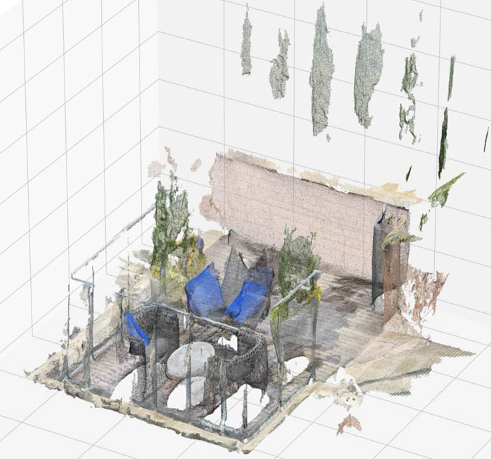
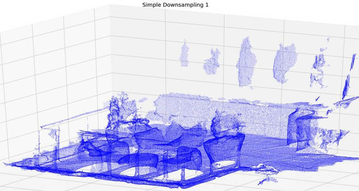
The data we use in this post is a scan of an apartment building rooftop generated using the 3D Scanner App on an iPhone12 Pro. The app allows you to use the built-in LiDAR scanners on mobile devices to scan a given area and export a point cloud file. In this case, the point cloud data is in xyzrgb format, an accepted format for a Ground Truth point cloud. For more information about the data types allowed in a Ground Truth point cloud, see Accepted Raw 3D Data Formats.

The following image shows our 3D scan.

Methods

We first walk through a few approaches to reduce dataset size for labeling point clouds: tiling, fixed step sample, and voxel mean. We demonstrate why downsampling techniques can increase your labeling throughput without significantly sacrificing annotation quality, and then we demonstrate how to use labels created on the downsampled point cloud and apply them to your original point cloud with an upsampling approach.

Downsampling approaches

Downsampling is taking your full-size dataset and either choosing a subset of points from it to label, or creating a representative set of new points that aren’t necessarily in the original dataset, but are close enough to allow labeling.

Tiling

One naive approach is to break your point cloud space into 3D cubes, otherwise known as voxels, of (for example) 500,000 points each that are labeled independently in parallel. This approach, called tiling, effectively reduces the scene size for labeling.

However, it can greatly increase labeling time and costs, because a typical 8-million-point scene may need to be broken up into over 16 sub-scenes. The large number of independent tasks that result from this method means more annotator time is spent on context switching between tasks, and workers may lose context when the scene is too small, resulting in mislabeled data.

Fixed step sample

An alternative approach is to select or create a reduced number of points by a linear subsample, called a fixed step sample. Let’s say you want to hit a target of 500,000 points (we have observed this is generally renderable on a consumer laptop—see Accepted Raw 3D Data Format), but you have a point cloud with 10 million points. You can calculate your step size as step = 10,000,000 / 500,000 = 20. After you have a step size, you can select every 20th point in your dataset, creating a new point cloud. If your point cloud data is of high enough density, labelers should still be able to make out any relevant features for labeling even though you may only have 1 point for every 20 in the original scene.

The downside of this approach is that not all points contribute to the final downsampled result, meaning that if a point is one of few important ones, but not part of the sample, your annotators may miss the feature entirely.

Voxel mean

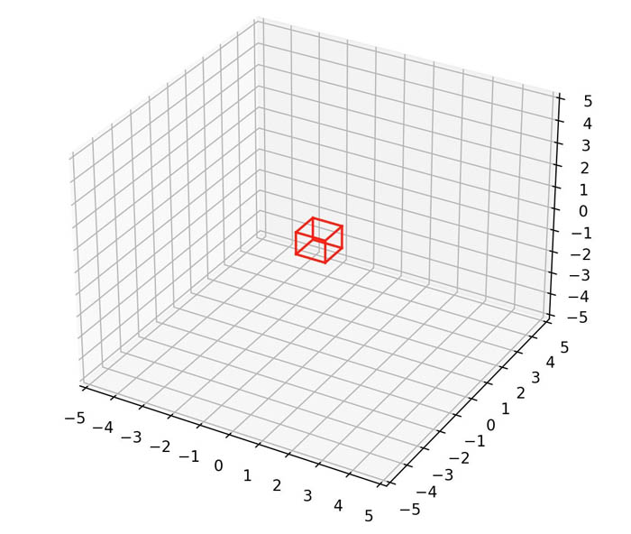
An alternate form of downsampling that uses all points to generate a downsampled point cloud is to perform grid filtering. Grid filtering means you break the input space into regular 3D boxes (or voxels) across the point cloud and replace all points within a voxel with a single representative point (the average point, for example). The following diagram shows an example voxel red box.

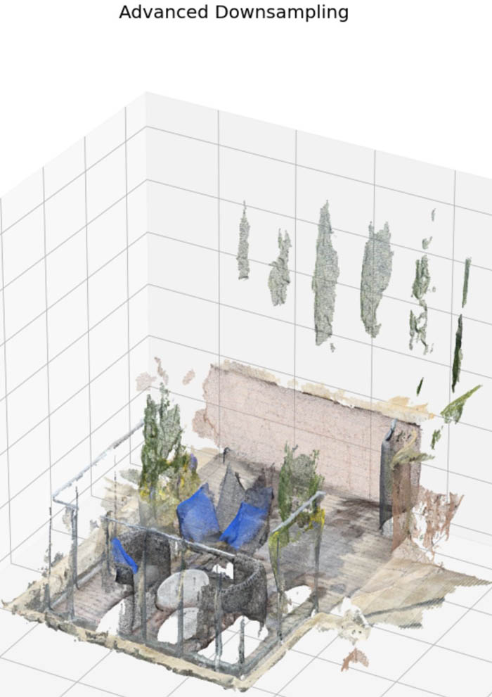
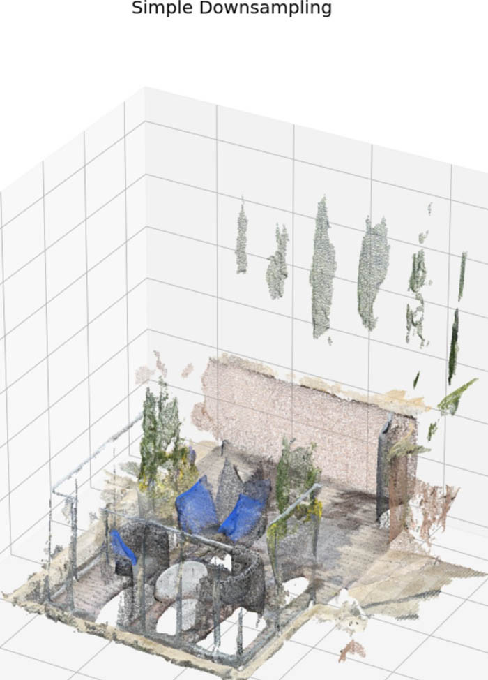
If no points exist from the input dataset within a given voxel, no point is added to the downsampled point cloud for that voxel. Grid filtering differs from a fixed step sample because you can use it to reduce noise and further tune it by adjusting the kernel size and averaging function to result in slightly different final point clouds. The following point clouds show the results of simple (fixed step sample) and advanced (voxel mean) downsampling. The point cloud downsampled using the advanced method is smoother, this is particularly noticeable when comparing the red brick wall in the back of both scenes.

Upsampling approach

After downsampling and labeling your data, you may want to see the labels produced on the smaller, downsampled point cloud projected onto the full-size point cloud, which we call upsampling. Object detection or tracking jobs don’t require post-processing to do this. Labels in the downsampled point cloud (like cuboids) are directly applicable to the larger point cloud because they’re defined in a world coordinate space shared by the full-size point cloud (x, y, z, height, width, length). These labels are minimally susceptible to very small errors along the boundaries of objects when a boundary point wasn’t in the downsampled dataset, but such occasional and minor errors are outweighed by the number of extra, correctly labeled points within the cuboid that can also be trained on.

For 3D point cloud semantic segmentation jobs, however, the labels aren’t directly applicable to the full-size dataset. We only have a subset of the labels, but we want to predict the rest of the full dataset labels based on this subset. To do this, we can use a simple K-Nearest Neighbors (K-NN) classifier with the already labeled points serving as the training set. K-NN is a simple supervised ML algorithm that predicts the label of a point using the “K” closest labeled points and a weighted vote. With K-NN, we can predict the point class of the rest of the unlabeled points in the full-size dataset based on the majority class of the three closest (by Euclidean distance) points. We can further refine this approach by varying the hyperparameters of a K-NN classifier, like the number of closest points to consider as well as the distance metric and weighting scheme of points.

After you map the sample labels to the full dataset, you can visualize tiles within the full-size dataset to see how well the upsampling strategy worked.

Now that we’ve reviewed the methods used in this post, we demonstrate these techniques in a SageMaker notebook on an example semantic segmentation point cloud scene.

Prerequisites

To walk through this solution, you need the following:

  • An AWS account.
  • A notebook AWS Identity and Access Management (IAM) role with the permissions required to complete this walkthrough. Your IAM role must have the following AWS managed policies attached:
    • AmazonS3FullAccess
    • AmazonSageMakerFullAccess
  • An Amazon Simple Storage Service (Amazon S3) bucket where the notebook artifacts (input data and labels) are stored.
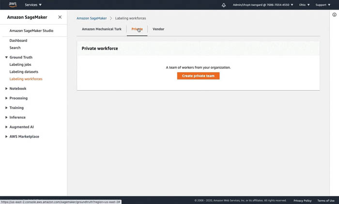
  • A SageMaker work team. For this post, we use a private work team. You can create a work team on the SageMaker console.

Notebook setup

We use the notebook ground_truth_annotation_dense_point_cloud_tutorial.ipynb in the SageMaker Examples section of a notebook instance to demonstrate these downsampling and upsampling approaches. This notebook contains all code required to perform preprocessing, labeling, and postprocessing.

To access the notebook, complete the following steps:

  1. Create a notebook instance. You can use the instance type, ml.t2.xlarge, to launch the notebook instance. Please choose an instance with at least 16 GB of RAM.
    1. You need to use the notebook IAM role you created early. This role allows your notebook to upload your dataset to Amazon S3 and call the solution APIs.
  2. Open Jupyter Lab or Jupyter to access your notebook instance.
  3. In Jupyter, choose the SageMaker Examples In Jupyter Lab, choose the SageMaker icon.
  4. Choose Ground Truth Labeling Jobs and then choose the ipynb notebook.
  5. If you’re using Jupyter, choose Use to copy the notebook to your instance and run it. If you’re in Jupyter lab, choose Create a Copy.

Provide notebook inputs

First, we modify the notebook to add our private work team ARN and the bucket location we use to store our dataset as well as our labels.

Section 1: Retrieve the dataset and visualize the point cloud

We download our data by running Section 1 of our notebook, which downloads our dataset from Amazon S3 and loads the point cloud into our notebook instance. We download custom prepared data from an AWS owned bucket. An object called rooftop_12_49_41.xyz should be in the root of the S3 bucket. This data is a scan of an apartment building rooftop custom generated on a mobile device. In this case, the point cloud data is in xyzrgb format.

We can visualize our point cloud using the Matplotlib scatter3d function. The point cloud file contains all the correct points but isn’t rotated correctly. We can rotate the object around its axis by multiplying the point cloud by a rotation matrix. We can obtain a rotation matrix using scipy and specify the degree changes we want to make to each axis using the from_euler method:

!aws s3 cp s3://smgt-downsampling-us-east-1-322552456788/rooftop_12_49_41.xyz pointcloud.xyz

# Let's read our dataset into a numpy file
pc = np.loadtxt("pointcloud.xyz", delimiter=",")

print(f"Loaded points of shape {pc.shape}")

# playing with view of 3D scene

from scipy.spatial.transform import Rotation

def plot_pointcloud(pc, rot = [[30,90,60]], color=True, title="Simple Downsampling 1", figsize=(50,25), verbose=False):
    if rot:
        rot1 = Rotation.from_euler('zyx', [[30,90,60]], degrees=True)
        R1 = rot1.as_matrix()
        if verbose:
            print('Rotation matrix:','n',R1)
            
        # matrix multiplication between our rotation matrix and pointcloud 
        pc_show = np.matmul(R1, pc.copy()[:,:3].transpose() ).transpose()
        if color:
            try:
                rot_color1 = np.matmul(R1, pc.copy()[:,3:].transpose() ).transpose().squeeze()
            except:
                rot_color1 = np.matmul(R1, np.tile(pc.copy()[:,3],(3,1))).transpose().squeeze()
    else:
        pc_show = pc
            
    fig = plt.figure( figsize=figsize)
    ax = fig.add_subplot(111, projection="3d")
    ax.set_title(title, fontdict={'fontsize':20})
    if color:
        ax.scatter(pc_show[:,0], pc_show[:,1], pc_show[:,2], c=rot_color1[:,0], s=0.05)
    else:
        ax.scatter(pc_show[:,0], pc_show[:,1], pc_show[:,2], c='blue', s=0.05)
        
# rotate in z direction 30 degrees, y direction 90 degrees, and x direction 60 degrees
rot1 = Rotation.from_euler('zyx', [[30,90,60]], degrees=True) 
print('Rotation matrix:','n', rot1.as_matrix())

plot_pointcloud(pc, rot = [[30,90,60]], color=True, title="Full pointcloud", figsize=(50,30))

Section 2: Downsample the dataset

Next, we downsample the dataset to less than 500,000 points, which is an ideal number of points for visualizing and labeling. For more information, see the Point Cloud Resolution Limits in Accepted Raw 3D Data Formats. Then we plot the results of our downsampling by running Section 2.

As we discussed earlier, the simplest form of downsampling is to choose values using a fixed step size based on how large we want our resulting point cloud to be.

A more advanced approach is to break the input space into cubes, otherwise known as voxels, and choose a single point per box using an averaging function. A simple implementation of this is shown in the following code.

You can tune the target number of points and box size used to see the reduction in point cloud clarity as more aggressive downsampling is performed.

#Basic Approach
target_num_pts = 500_000
subsample = int(np.ceil(len(pc) / target_num_pts))
pc_downsample_simple = pc[::subsample]
print(f"We've subsampled to {len(pc_downsample_simple)} points")

#Advanced Approach
boxsize = 0.013 # 1.3 cm box size.
mins = pc[:,:3].min(axis=0)
maxes = pc[:,:3].max(axis=0)
volume = maxes - mins
num_boxes_per_axis = np.ceil(volume / boxsize).astype('int32').tolist()
num_boxes_per_axis.extend([1])

print(num_boxes_per_axis)

# For each voxel or "box", use the mean of the box to chose which points are in the box.
means, _, _ = scipy.stats.binned_statistic_dd(
    pc[:,:4],
    [pc[:,0], pc[:,1], pc[:,2], pc[:,3]], 
    statistic="mean",
    bins=num_boxes_per_axis,
)
x_means = means[0,~np.isnan(means[0])].flatten()
y_means = means[1,~np.isnan(means[1])].flatten()
z_means = means[2,~np.isnan(means[2])].flatten()
c_means = means[3,~np.isnan(means[3])].flatten()
pc_downsample_adv = np.column_stack([x_means, y_means, z_means, c_means])
print(pc_downsample_adv.shape)

Section 3: Visualize the 3D rendering

We can visualize point clouds using a 3D scatter plot of the points. Although our point clouds have color, our transforms have different effects on color, so comparing them in a single color provides a better comparison. We can see that the advanced voxel mean method creates a smoother point cloud because averaging has a noise reduction effect. In the following code, we can look at our point clouds from two separate perspectives by multiplying our point clouds by different rotation matrices.

When you run Section 3 in the notebook, you also see a comparison of a linear step approach versus a box grid approach, specifically in how the box grid filter has a slight smoothing effect on the overall point cloud. This smoothing could be important depending on the noise level of your dataset. Modifying the grid filtering function from mean to median or some other averaging function can also improve the final point cloud clarity. Look carefully at the back wall of the simple (fixed step size) and advanced (voxel mean) downsampled examples, notice the smoothing effect the voxel mean method has compared to the fixed step size method.

rot1 = Rotation.from_euler('zyx', [[30,90,60]], degrees=True)
R1 = rot1.as_matrix()

simple_rot1 = pc_downsample_simple.copy()
simple_rot1 = np.matmul(R1, simple_rot1[:,:3].transpose() ).transpose()
advanced_rot1 = pc_downsample_adv.copy()
advanced_rot1 = np.matmul(R1, advanced_rot1[:,:3].transpose() ).transpose()

fig = plt.figure( figsize=(50, 30))
ax = fig.add_subplot(121, projection="3d")
ax.set_title("Simple Downsampling 1", fontdict={'fontsize':20})
ax.scatter(simple_rot1[:,0], simple_rot1[:,1], simple_rot1[:,2], c='blue', s=0.05)
ax = fig.add_subplot(122, projection="3d")
ax.set_title("Voxel Mean Downsampling 1", fontdict={'fontsize':20})
ax.scatter(advanced_rot1[:,0], advanced_rot1[:,1], advanced_rot1[:,2], c='blue', s=0.05)

# to look at any of the individual pointclouds or rotate the pointcloud, use the following function

plot_pointcloud(pc_downsample_adv, rot = [[30,90,60]], color=True, title="Advanced Downsampling", figsize=(50,30))

Section 4: Launch a Semantic Segmentation Job

Run Section 4 in the notebook to take this point cloud and launch a Ground Truth point cloud semantic segmentation labeling job using it. These cells generate the required input manifest file and format the point cloud in a Ground Truth compatible representation.

To learn more about the input format of Ground Truth as it relates to point cloud data, see Input Data and Accepted Raw 3D Data Formats.

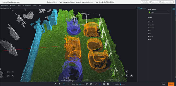
In this section, we also perform the labeling in the worker portal. We label a subset of the point cloud to have some annotations to perform upsampling with. When the job is complete, we load the annotations from Amazon S3 into a NumPy array for our postprocessing. The following is a screenshot from the Ground Truth point cloud semantic segmentation tool.

Section 5: Perform label upsampling

Now that we have the downsampled labels, we train a K-NN classifier from SKLearn to predict the full dataset labels by treating our annotated points as training data and performing inference on the remainder of the unlabeled points in our full-size point cloud.

You can tune the number of points used as well as the distance metric and weighting scheme to influence how label inference is performed. If you label a few tiles in the full-size dataset, you can use those labeled tiles as ground truth to evaluate the accuracy of the K-NN predictions. You can then use this accuracy metric for hyperparameter tuning of K-NN or to try different inference algorithms to reduce your number of misclassified points between object boundaries, resulting in the lowest possible in-sample error rate. See the following code:

# There's a lot of possibility to tune KNN further
# 1) Prevent classification of points far away from all other points (random unfiltered ground point)
# 2) Perform a non-uniform weighted vote
# 3) Tweak number of neighbors
knn = KNeighborsClassifier(n_neighbors=3)
print(f"Training on {len(pc_downsample_adv)} labeled points")
knn.fit(pc_downsample_adv[:,:3], annotations)

print(f"Upsampled to {len(pc)} labeled points")
annotations_full = knn.predict(pc[:,:3])

Section 6: Visualize the upsampled labels

Now that we have performed upsampling of our labeled data, we can visualize a tile of the original full-size point cloud. We aren’t rendering all of the full-size point cloud because that may prevent our visualization tool from rendering. See the following code:

pc_downsample_annotated = np.column_stack((pc_downsample_adv[:,:3], annotations))
pc_annotated = np.column_stack((pc[:,:3], annotations_full))

labeled_area = pc_downsample_annotated[pc_downsample_annotated[:,3] != 255]
min_bounds = np.min(labeled_area, axis=0)
max_bounds = np.max(labeled_area, axis=0)

min_bounds = [-2, -2, -4.5, -1]
max_bounds = [2, 2, -1, 256]

def extract_tile(point_cloud, min_bounds, max_bounds):
    return point_cloud[
        (point_cloud[:,0] > min_bounds[0])
        & (point_cloud[:,1] > min_bounds[1])
        & (point_cloud[:,2] > min_bounds[2])
        & (point_cloud[:,0] < max_bounds[0])
        & (point_cloud[:,1] < max_bounds[1])
        & (point_cloud[:,2] < max_bounds[2])
    ]


tile_downsample_annotated = extract_tile(pc_downsample_annotated, min_bounds, max_bounds)
tile_annotated = extract_tile(pc_annotated, min_bounds, max_bounds)

rot1 = Rotation.from_euler('zyx', [[30,90,60]], degrees=True)
R1 = rot1.as_matrix()

down_rot = tile_downsample_annotated.copy()
down_rot = np.matmul(R1, down_rot[:,:3].transpose() ).transpose()
down_rot_color = np.matmul(R1, np.tile(tile_downsample_annotated.copy()[:,3],(3,1))).transpose().squeeze()

full_rot = tile_annotated.copy()
full_rot = np.matmul(R1, full_rot[:,:3].transpose() ).transpose()
full_rot_color = np.matmul(R1, np.tile(tile_annotated.copy()[:,3],(3,1))).transpose().squeeze()


fig = plt.figure(figsize=(50, 20))
ax = fig.add_subplot(121, projection="3d")
ax.set_title("Downsampled Annotations", fontdict={'fontsize':20})
ax.scatter(down_rot[:,0], down_rot[:,1], down_rot[:,2], c=down_rot_color[:,0], s=0.05)
ax = fig.add_subplot(122, projection="3d")
ax.set_title("Upsampled Annotations", fontdict={'fontsize':20})
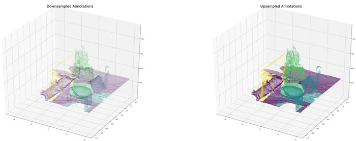
ax.scatter(full_rot[:,0], full_rot[:,1], full_rot[:,2], c=full_rot_color[:,0], s=0.05)

Because our dataset is dense, we can visualize the upsampled labels within a tile to see the downsampled labels upsampled to the full-size point cloud. Although a small number of misclassifications may exist along boundary regions between objects, you also have many more correctly labeled points in the full-size point cloud than the initial point cloud, meaning your overall ML accuracy may improve.

Cleanup

Notebook instance: you have two options if you do not want to keep the created notebook instance running. If you would like to save it for later, you can stop rather than deleting it.

  • To stop a notebook instance: click the Notebook instances link in the left pane of the SageMaker console home page. Next, click the Stop link under the ‘Actions’ column to the left of your notebook instance’s name. After the notebook instance is stopped, you can start it again by clicking the Start link. Keep in mind that if you stop rather than delete it, you will be charged for the storage associated with it.
  • To delete a notebook instance: first stop it per the instruction above. Next, click the radio button next to your notebook instance, then select Delete from the Actions drop down menu.

Conclusion

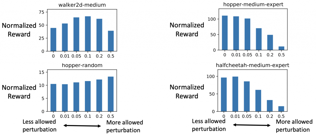
Downsampling point clouds can be a viable method when preprocessing data for object detection and object tracking labeling. It can reduce labeling costs while still generating high-quality output labels, especially for 3D object detection and tracking tasks. In this post, we demonstrated how the downsampling method can affect the clarity of the point cloud for workers, and showed a few approaches that have tradeoffs based on the noise level of the dataset.

Finally, we showed that you can perform 3D point cloud semantic segmentation jobs on downsampled datasets and map the labels to the full-size point cloud through in-sample prediction. We accomplished this by training a classifier to do inference on the remaining full dataset size points, using the already labeled points as training data. This approach enables cost-effective labeling of highly dense point cloud scenes while still maintaining good overall label quality.

Test out this notebook with your own dense point cloud scenes in Ground Truth, try out new downsampling techniques, and even try new models beyond K-NN for final in-sample prediction to see if downsampling and upsampling techniques can reduce your labeling costs.


About the Authors

 Vidya Sagar Ravipati is a Deep Learning Architect at the Amazon ML Solutions Lab, where he leverages his vast experience in large-scale distributed systems and his passion for machine learning to help AWS customers across different industry verticals accelerate their AI and cloud adoption. Previously, he was a Machine Learning Engineer in Connectivity Services at Amazon who helped to build personalization and predictive maintenance platforms.


Isaac Privitera is a Machine Learning Specialist Solutions Architect and helps customers design and build enterprise-grade computer vision solutions on AWS. Isaac has a background in using machine learning and accelerated computing for computer vision and signals analysis. Isaac also enjoys cooking, hiking, and keeping up with the latest advancements in machine learning in his spare time.


Jeremy Feltracco is a Software Development Engineer with the Amazon ML Solutions Lab at Amazon Web Services. He uses his background in computer vision, robotics, and machine learning to help AWS customers accelerate their AI adoption.

Read More

Adaptive Framework for On-device Recommendation

Posted by Ellie Zhou, Tian Lin, Shuangfeng Li and Sushant Prakash

Introduction & Motivation

We are excited to announce an adaptive framework to build on-device recommendation ML solutions with your own data and advanced user modeling architecture.

After the previously open-sourced on-device recommendation solution, we received a lot of interest from the community on introducing on-device recommender AI. Motivated and inspired by the feedback, we considered various use cases, and created a framework that could generate TensorFlow Lite recommendation models accommodating different kinds of data, features, and architectures to improve the previous models.

Benefits of this framework:

  • Flexible: The adaptive framework allows users to create a model in a configurable way.
  • Better model representation: To improve the previous model, our new recommendation models can utilize multiple kinds of features than a single feature.

Personalized recommendations play an increasingly important role in digital life nowadays. With more and more user actions being moved to edge devices, supporting recommenders on-device becomes an important direction. Compared with conventional pure server-based recommenders, the on-device solution has unique advantages, such as protecting users’ privacy, providing fast reaction to on-device user actions, leveraging lightweight TensorFlow Lite inference, and bypassing network dependency. We welcome you to try out this framework and create recommendation experience in your applications.

In this article, we will

  • Introduce the improved model architecture and framework adaptivity.
  • Walk you through how to utilize the framework step-by-step.
  • Provide insights based on research done with a public dataset.

Please find more details on TensorFlow website.

Model

A recommendation model typically predicts users’ future activities, based on users’ previous activities. Our framework supports models using context information to do the prediction, which can be described in the following architecture:

recommendation code structure
Figure 1: An illustration of the configurable recommendation model. Each module is created according to the user-defined configuration.

At the context side, representations of all user activities are aggregated by the encoder to generate the context embedding. We support three different types of encoders: 1) bag-of-words (a.k.a. BOW), 2) 1-D convolution (a.k.a. CNN), and 3) LSTM. At the label side, the label item as positive and all other items in the vocabulary as negatives will be encoded to vectors as well. Context and label embeddings are combined with a dot product and fed to the loss of softmax cross entropy.

Inside the framework, we encapsulate tf.keras layers for ContextEncoder, LabelEncoder and DotProductSimilarity as key components in RecommendationModel.

To model each user activity, we could use the ID of the activity item (called ID-based), or multiple features of the item (called feature-based), or a combination of both. The feature-based model utilizing multiple features to collectively encode users’ behavior. With our framework, you could create either ID-based or feature-based models in a configurable way.

Similar to the last version, a TensorFlow Lite model will be exported after training which can directly provide top-K predictions among the recommendation candidates.

Step-by-step

To demonstrate the new adaptive framework, we trained a on-device movie recommendation model with MovieLens dataset using multiple features, and integrated it in the demo app. (Both the model and the app are for demonstration purposes only.) The MovieLens 1M dataset contains ratings from 6039 users across 3951 movies, with each user rating only a small subset of movies.

Let’s look at how to use the framework step-by-step in this notebook.

(a) Environment preparation

git clone https://github.com/tensorflow/examples
cd examples/lite/examples/recommendation/ml/
pip install -r requirements.txt

(b) Prepare training data

Please prepare your training data reference to the movielens example generation file. Would like to note that TensorFlow Lite input features are expected to be FixedLenFeature, please pad or truncate your features, and set up feature lengths in input configuration. Feel free to use the following command to process the example dataset.

python -m data.example_generation_movielens 
--data_dir=data/raw
--output_dir=data/examples
--min_timeline_length=3
--max_context_length=10
--max_context_movie_genre_length=32
--min_rating=2
--train_data_fraction=0.9
--build_vocabs=True

MovieLens data contains ratings.dat (columns: UserID, MovieID, Rating, Timestamp), and movies.dat (columns: MovieID, Title, Genres). The example generation script takes both files, only keep ratings higher than 2, form user movie interaction timelines, sample activities as labels and previous user activities as the context for prediction. Please find the generated tf.Example:

0 : {
features: {
feature: {
key : "context_movie_id"
value: { int64_list: { value: [ 1124, 2240, 3251, ..., 1268 ] } }
}
feature: {
key : "context_movie_rating"
value: { float_list: {value: [ 3.0, 3.0, 4.0, ..., 3.0 ] } }
}
feature: {
key : "context_movie_year"
value: { int64_list: { value: [ 1981, 1980, 1985, ..., 1990 ] } }
}
feature: {
key : "context_movie_id"
value: { int64_list: { value: [ 1124, 2240, 3251, ..., 1268 ] } }
}
feature: {
key : "context_movie_genre"
value: { bytes_list: { value: [ "Drama", "Drama", "Mystery", ..., "UNK" ] } }
}
feature: {
key : "label_movie_id"
value: { int64_list: { value: [ 3252 ] } }
}
}
}

(c) Create input config

Once data prepared, please set up input configuration, e.g. this is one example configuration for movielens movie recommendation model.

activity_feature_groups {
features {
feature_name: "context_movie_id"
feature_type: INT
vocab_size: 3953
embedding_dim: 8
feature_length: 10
}
features {
feature_name: "context_movie_rating"
feature_type: FLOAT
feature_length: 10
}
encoder_type: CNN
}
activity_feature_groups {
features {
feature_name: "context_movie_genre"
feature_type: STRING
vocab_name: "movie_genre_vocab.txt"
vocab_size: 19
embedding_dim: 4
feature_length: 32
}
encoder_type: CNN
}
label_feature {
feature_name: "label_movie_id"
feature_type: INT
vocab_size: 3953
embedding_dim: 8
feature_length: 1
}

(d) Train model

The model trainer will construct the recommendation model based on the input config, with a simple interface.

python -m model.recommendation_model_launcher -- 
--training_data_filepattern "data/examples/train_movielens_1m.tfrecord"
--testing_data_filepattern "data/examples/test_movielens_1m.tfrecord"
--model_dir "model/model_dir"
--vocab_dir "data/examples"
--input_config_file "configs/sample_input_config.pbtxt"
--batch_size 32
--learning_rate 0.01
--steps_per_epoch 2
--num_epochs 2
--num_eval_steps 2
--run_mode "train_and_eval"
--gradient_clip_norm 1.0
--num_predictions 10
--hidden_layer_dims "32,32"
--eval_top_k "1,5"
--conv_num_filter_ratios "2,4"
--conv_kernel_size 4
--lstm_num_units 16

Inside the recommendation model, core components are packaged up to keras layers (context_encoder.py, label_encoder.py and dotproduct_similarity.py), each of which could be utilized by itself. The following diagram illustrates the code structure:

An example of model architecture using context information to predict the next movie.
Figure 2: An example of model architecture using context information to predict the next movie. The inputs are the history of (a) movie IDs, (b) ratings and (c) genres, which is specified by the config mentioned above.

With the framework, you can directly execute the model training launcher with command:

python -m model.recommendation_model_launcher 
--input_config_file "configs/sample_input_config.pbtxt"
--vocab_dir "data/examples"
--run_mode "export"
--checkpoint_path "model/model_dir/ckpt-1000"
--num_predictions 10
--hidden_layer_dims "32,32"
--conv_num_filter_ratios "2,4"
--conv_kernel_size 4
--lstm_num_units 16

The inference code after exporting to TensorFlow Lite can be found in the notebook, and we refer readers to check out the details there.

Framework Adaptivity

Our framework provides a protobuf interface, through which feature groups, types and other information can be configured to build models accordingly. With the interface, you can configure:

  • Features

    The framework generically categorizes features into 3 types: integer, string, and float. Embedding spaces will be created for both integer and string features, hence, embedding dimension, vocabulary name and size need to be specified. Float feature values will be directly used. Besides, for on-device models, we suggest to use fixed length features which can be configured directly.

message Feature {
optional string feature_name = 1;

// Supported feature types: STRING, INT, FLOAT.
optional FeatureType feature_type = 2;

optional string vocab_name = 3;

optional int64 vocab_size = 4;

optional int64 embedding_dim = 5;

optional int64 feature_length = 6;
}
  • Feature groups

    One feature for one user activity may have multiple values. For instance, one movie can belong to multiple categories, each movie will have multiple genre feature values. To handle the different feature shapes, we introduced the “feature group” to combine features as a group . The features with the same length can be put in the same feature group to be encoded together. Inside input config, you can set up global feature groups and activity feature groups.

message FeatureGroup {
repeated Feature features = 1;

// Supported encoder types: BOW, CNN, LSTM.
optional EncoderType encoder_type = 2;
}
  • Input config

    You can use the input config interface to set up all the features and feature groups together.

message InputConfig {
repeated FeatureGroup global_feature_groups = 1;

repeated FeatureGroup activity_feature_groups = 2;

optional Feature label_feature = 3;
}

The input config is utilized by both input_pipeline.py and recommendation_model.py to process training data to tf.data.Dataset and construct the model accordingly. Inside ContexEncoder, FeatureGroupEncoders will be created for all feature groups, and used to compute feature group embeddings from input features. Concatenated feature group embeddings will be fed through top hidden layers to get the final context embedding. Worth noting that the final context embedding and label embedding dimensions should be equal.

Please check out the different model graphs produced with the different input configurations in the Appendix section.

Experiments and Analysis

We take this opportunity to analyze the performance of ID-based and feature-based models with various configurations, and provide some empirical results.

For the ID-based model, only movie_id is used as the input feature. And for the feature-based model, both movie_id and movie_genre features are used. Both types of models are experimented with 3 encoder types (BOW/CNN/LSTM) and 3 context history lengths (10/50/100).

Comparison between ID-based and Feature-based models.
Comparison between ID-based and Feature-based models. We compare them on BOW/CNN/LSTM encoders and context history lengths 10/50/100.

Since MovieLens dataset is an experimental dataset with ~4000 candidate movies and 19 movie genres, hence we scaled down embedding dimensions in the experiments to simulate the production scenario. For the above experiment result chart, ID embedding dimension is set to 8, and movie genre embedding dimension is set to 4. If we take the context10_cnn as an example, the feature-based model outperforms the ID-based model by 58.6%. Furthermore, the on average results show that feature-based models outperforms by 48.35%. Therefore, In this case, the feature-based model outperforms the ID-based model, because movie_genre feature introduces additional information to the model.

Besides, underlying features of candidate items mostly have a smaller vocabulary size, hence smaller embedding spaces as well. For instance,the movie genre vocabulary is much smaller than the movie ID vocabulary. In this case, utilizing underlying features could reduce the memory size of the model, which is more on-device friendly.

Acknowledgement

Special thanks to Cong Li, Josh Gordon, Khanh LeViet‎, Arun Venkatesan and Lawrence Chan for providing valuable suggestions to this work.

Read More

Update Complete: GFN Thursday Brings New Features, Games and More

No Thursday is complete without GFN Thursday, our weekly celebration of the news, updates and great games GeForce NOW members can play — all streaming from the cloud across nearly all of your devices.

This week’s exciting updates to the GeForce NOW app and experience Include updated features, faster session loading and a bunch of new games joining the GFN library.

… Better, Faster, Stronger

There’s a lot happening behind the scenes as our team continuously works to improve your cloud-gaming experience with each session.

Our cloud-gaming engineers work to further improve your streaming sessions, optimize games and develop new features. We also continually refine the user experience in the GeForce NOW app, which is now rolling out version 2.0.29 with several improvements.

Game in the Fast Lane

From the Settings pane in the GeForce NOW app, you can link your Epic Games Store account to take advantage of some new features.

One feature we’re currently testing with our Founders and Priority members is preloading, which loads parts of your game before you arrive so your launch times will be faster. Members testing this feature should see sessions launch up to a minute faster from the moment they click play in the GeForce NOW app. Free members are not guaranteed preloaded sessions and may see slightly longer startup times.

To enable the benefits of preloading, we’re also testing a new account linking feature which lets you play games without having to login into your game store account. Both the preloading and account linking features are currently enabled for Fortnite’s PC build on GeForce NOW. We anticipate an expansion of these features to more GeForce NOW games in the future.

PC, macOS and Chromebook users can enable the new account linking features from a new tile on the My Library row in-app. This takes you to the Settings pane, where you can turn on account linking for Fortnite under Connections. Once complete, you won’t need to log in to your Epic Account to play Fortnite’s PC build on any other supported GeForce NOW platform, and you’ll be eligible for preloaded sessions.

Find What You’re Looking For

We’re also improving search results in the app to make managing libraries easier and get members in games faster. Searching for games to add to libraries will now return full page search results, providing easier access to the game’s details and a quicker way to add it to your library.

The newest version of the GeForce NOW app includes improved search, account linking for Epic Games Store, and a whole lot more.

If you’re playing on GeForce NOW from a Chrome browser, we’ve recently added our in-game overlay.  The overlay lets members configure many in-stream features, such as FreeStyle filters, network labels, microphone toggles and ending game sessions. To bring up the overlay, using Ctrl + G for PC and Chromebook, or CMD + G for macOS.

And no GeForce NOW app update would be complete without squashed bugs. To get the full lowdown, check out the version 2.0.29 Release Highlights from the Settings pane in the app.

These updates are just a few of the improvements we’re working on. We have a ton more in store, and every update is designed to make sure that when GFN members play their favorite PC games from our cloud servers, they’re getting the best possible experience.

Rolling in the Deep (Silver)

We recently spoke with our friends at Deep Silver about new updates coming for KING Art Games’ Iron Harvest and 4A Games’ Metro Exodus: Enhanced Edition, both of which will be supported on GeForce NOW. Catch up on all the details here.

Get Your Game On

The latest in the classic R-Type series comes to GeForce NOW this week.

Finally, below are the games joining the GeForce NOW library this week. 

What do you think of the newest GeForce NOW updates? Let us know on Twitter or in the comments below.

The post Update Complete: GFN Thursday Brings New Features, Games and More appeared first on The Official NVIDIA Blog.

Read More