Carnegie Mellon University is proud to present 194 papers at the 38th conference on Neural Information Processing Systems (NeurIPS 2024), held from December 10-15 at the Vancouver Convention Center. Here is a quick overview of the areas our researchers are working on:

Here are some of our top collaborator institutions:

Table of Contents
- Oral Papers
- Spotlight Papers
- Poster Papers
- Causality
- Computational Biology
- Computer Vision
- Computer Vision (Image Generation)
- Computer Vision (Video Generation)
- Computer Vision (Video Understanding)
- Data-centric AI
- Data-centric AI (Data Augmentation)
- Data-centric AI (Data-centric AI Methods And Tools)
- Deep Learning (Algorithms)
- Deep Learning (Attention Mechanisms)
- Deep Learning (Everything Else)
- Deep Learning (Representation Learning)
- Deep Learning (Robustness)
- Fairness
- Generative Models
- Generative Models (Diffusion Models)
- Generative Models (In Context Learning)
- Generative Models (Misc)
- Generative Models (Reasoning)
- Graph Neural Networks
- Human-computer Interaction
- Interpretability
- Language (Dialogue)
- Language (Generation)
- Language (Knowledge)
- Learning Theory
- Miscellaneous Aspects Of Machine Learning (General Machine Learning Techniques)
- Miscellaneous Aspects Of Machine Learning (Supervised Learning)
- Multimodal Models
- Neuroscience, Cognitive Science
- Online Learning
- Optimization
- Optimization (Convex)
- Optimization (Large Scale, Parallel And Distributed)
- Optimization (Learning For Optimization)
- Other
- Privacy
- Reinforcement Learning (Batch Offline)
- Reinforcement Learning (Everything Else)
- Reinforcement Learning (Multi-agent)
- Reinforcement Learning (Planning)
- Robotics
- Theory (Everything Else)
- Theory (Game Theory)
- Theory (Reinforcement Learning And Planning)
- Time Series
- Trustworthy Machine Learning
Oral Papers
Stylus: Automatic Adapter Selection for Diffusion Models
This paper explores an alternative approach to generating high-fidelity, customized images at reduced costs using fine-tuned adapters instead of simply scaling base models with additional data or parameters. Over time, the open-source community has created a large collection of more than 100,000 adapters—small modules that fine-tune base models for specific tasks. However, many of these adapters are highly customized and lack clear descriptions, making them challenging to use effectively. To address this, the paper introduces Stylus, a system designed to match prompts with relevant adapters and automatically compose them for better image generation. Building on recent research showing the benefits of combining multiple adapters, Stylus uses a three-stage process: summarizing adapters with improved descriptions and embeddings, retrieving relevant adapters, and composing adapters based on prompt keywords to ensure a strong match. The authors also present StylusDocs, a curated dataset of 75,000 adapters with pre-computed embeddings, for evaluation. Testing Stylus on popular Stable Diffusion checkpoints shows that it achieves better CLIP/FID Pareto efficiency and is twice as preferred by human and multimodal evaluators compared to the base model.
The Sample-Communication Complexity Trade-off in Federated Q-Learning
This work examines the problem of Federated Q-learning, where multiple agents collaboratively learn the optimal Q-function for an unknown infinite-horizon Markov Decision Process with finite state and action spaces. The focus is on understanding the trade-off between sample complexity (the number of data samples needed for learning) and communication complexity (the amount of data exchanged between agents) for intermittent communication algorithms, a commonly used approach in federated settings.
The authors first establish a fundamental limitation: any Federated Q-learning algorithm that achieves linear speedup in sample complexity relative to the number of agents must incur a communication cost of at least Ω(1/1−γ), where γ is the discount factor. They then introduce a new algorithm, Fed-DVR-Q, which is the first to achieve both optimal sample complexity and communication complexity simultaneously. Together, these results provide a comprehensive understanding of the trade-offs between sample and communication efficiency in Federated Q-learning.
Spotlight Papers
Aligner Encoders: Self-Attention Transformers Can Be Self-Transducers
The paper introduces a new transformer-based approach to automatic speech recognition (ASR) that simplifies the alignment process between audio input and text output. Unlike traditional models, the encoder itself aligns audio information internally, reducing the complexity of decoding. The proposed “Aligner-Encoder” model combines efficient training techniques and a lightweight decoder, resulting in significantly faster performance while maintaining competitive accuracy. Notably, the alignment process is evident in the self-attention weights of the model, showcasing its ability to handle the task efficiently.
Approximating the Top Eigenvector in Random Order Streams
This work focuses on streaming algorithms for approximating the top eigenvector of a matrix when its rows are presented in a random order. The authors introduce a new algorithm that works efficiently when there is a sufficient gap between the largest and second-largest eigenvalues of the matrix. Their approach uses a small amount of memory, depending on the number of “heavy rows” (rows with large norms), and produces highly accurate results. They also show that using this heavy-row-based parameterization is necessary for achieving high accuracy and improve on prior methods by reducing the gap requirement for random-order streams, though their method assumes the rows are presented in a random order rather than any order.
Connecting Joint-Embedding Predictive Architecture with Contrastive Self-supervised Learning
Recent advancements in unsupervised visual representation learning have highlighted the Joint-Embedding Predictive Architecture (JEPA) as an effective method for extracting visual features from unlabeled images using masking strategies. However, JEPA faces two key challenges: its reliance on Exponential Moving Average (EMA) fails to prevent model collapse, and its predictions struggle to accurately capture the average representation of image patches. To address these issues, this work introduces C-JEPA, a new framework that combines JEPA with a variance-invariance-covariance regularization strategy called VICReg. This approach improves stability, prevents collapse, and ensures better learning of consistent representations. Experiments show that C-JEPA achieves faster convergence and higher performance on standard benchmarks when pre-trained on ImageNet-1K.
CooHOI: Learning Cooperative Human-Object Interaction with Manipulated Object Dynamics
This work addresses the challenge of enabling humanoid robots to collaborate on tasks like moving large furniture, which require coordination between multiple robots. Existing methods struggle due to a lack of motion capture data for multi-humanoid collaboration and the inefficiency of training multiple agents together. To overcome this, the authors introduce Cooperative Human-Object Interaction (CooHOI), a framework that uses a two-phase learning approach: first, individual humanoids learn object interaction skills from human motion data, and then they learn to work together using multi-agent reinforcement learning. By focusing on shared object dynamics and decentralized execution, the robots achieve coordination through implicit communication. Unlike previous tracking-based methods, CooHOI is efficient, does not rely on multi-humanoid motion data, and can easily scale to more participants and diverse object types.
DiffTOP: Differentiable Trajectory Optimization for Deep Reinforcement and Imitation Learning
This paper presents DiffTORI, a framework that uses differentiable trajectory optimization as a policy representation for reinforcement and imitation learning. Trajectory optimization, a common tool in control, is parameterized by a cost and a dynamics function, and recent advances now allow gradients of the loss to be computed with respect to these parameters. This enables DiffTORI to learn cost and dynamics functions end-to-end, addressing the “objective mismatch” in previous model-based RL methods by aligning the dynamics model with task performance. Benchmarking on robotic manipulation tasks with high-dimensional sensory inputs, DiffTORI demonstrates superior performance over prior methods, including feedforward policies, energy-based models, and diffusion models, across a wide range of reinforcement and imitation learning tasks.
Don’t Look Twice: Faster Video Transformers with Run-Length Tokenization
Video transformers are notoriously slow to train due to the large number of input tokens, many of which are repeated across frames. Existing methods to remove redundant tokens often introduce significant overhead or require dataset-specific tuning, limiting their practicality. This work introduces Run-Length Tokenization (RLT), a simple and efficient method inspired by run-length encoding, which identifies and removes repeated patches in video frames before inference. By replacing repeated patches with a single token and a positional encoding to reflect its duration, RLT reduces redundancy without requiring tuning or adding significant computational cost. It accelerates training by 30%, maintains baseline performance, and increases throughput by 35% with minimal accuracy loss, while reducing token counts by up to 80% on longer videos.
ICAL: Continual Learning of Multimodal Agents by Transforming Trajectories into Actionable Insights
This work introduces In-Context Abstraction Learning (ICAL), a method that enables large-scale language and vision-language models (LLMs and VLMs) to generate high-quality task examples from imperfect demonstrations. ICAL uses a vision-language model to analyze and improve inefficient task trajectories by abstracting key elements like causal relationships, object states, and temporal goals, with iterative refinement through human feedback. These improved examples, when used as prompts, enhance decision-making and reduce reliance on human input over time, making the system more efficient. ICAL outperforms state-of-the-art models in tasks like instruction following, web navigation, and action forecasting, demonstrating its ability to improve performance without heavy manual prompt engineering.
Is Your LiDAR Placement Optimized for 3D Scene Understanding?
This work focuses on improving the reliability of driving perception systems under challenging and unexpected conditions, particularly with multi-LiDAR setups. Most existing datasets rely on single-LiDAR systems and are collected in ideal conditions, making them insufficient for real-world applications. To address this, the authors introduce Place3D, a comprehensive pipeline that optimizes LiDAR placement, generates data, and evaluates performance. Their approach includes three key contributions: a new metric called the Surrogate Metric of the Semantic Occupancy Grids (M-SOG) for assessing multi-LiDAR configurations, an optimization strategy to improve LiDAR placements based on M-SOG, and the creation of a 280,000-frame dataset capturing both clean and adverse conditions. Experiments show that their optimized placements lead to significant improvements in tasks like semantic segmentation and 3D object detection, even in challenging scenarios with harsh weather or sensor failures.
Learn To be Efficient: Build Structured Sparsity in Large Language Models
The paper explores how Large Language Models (LLMs), known for their impressive capabilities but high computational costs, can be made more efficient. It highlights that while activation sparsity—where only some model parameters are used during inference—naturally occurs, current methods fail to maximize its potential during training. The authors propose a novel training algorithm, Learn-To-be-Efficient (LTE), that encourages LLMs to activate fewer neurons, striking a balance between efficiency and performance. Their approach, applicable to models beyond traditional ReLU-based ones, demonstrates improved results across various tasks and reduces inference latency by 25% for LLaMA2-7B at 50% sparsity.
Learning Social Welfare Functions
This work explores whether it is possible to understand or replicate a policymaker’s reasoning by analyzing their past decisions. The problem is framed as learning social welfare functions from the family of power mean functions. Two learning tasks are considered: one uses utility vectors of actions and their corresponding social welfare values, while the other uses pairwise comparisons of welfares for different utility vectors. The authors demonstrate that power mean functions can be learned efficiently, even when the social welfare data is noisy. They also propose practical algorithms for these tasks and evaluate their effectiveness.
Metric Transforms and Low Rank Representations of Kernels
The authors introduce a linear-algebraic tool based on group representation theory to solve three important problems in machine learning. First, they investigate fast attention algorithms for large language models and prove that only low-degree polynomials can produce the low-rank matrices required for subquadratic attention, thereby showing that polynomial-based approximations are essential. Second, they extend the classification of positive definite kernels from Euclidean distances to Manhattan distances, offering a broader foundation for kernel methods. Finally, they classify all functions that transform Manhattan distances into Manhattan distances, generalizing earlier work on Euclidean metrics and introducing new results about stable-rank-preserving functions with potential applications in algorithm design.
Sample-Efficient Private Learning of Mixtures of Gaussians
This work examines the problem of learning mixtures of Gaussians while ensuring approximate differential privacy. The authors demonstrate that it is possible to learn a mixture of k arbitrary d-dimensional Gaussians with significantly fewer samples than previous methods, achieving optimal performance when the dimensionality d is much larger than the number of components k. For univariate Gaussians, they establish the first optimal bound, showing that the sample complexity scales linearly with k, improving upon earlier methods that required a quadratic dependence on k. Their approach leverages advanced techniques, including the inverse sensitivity mechanism, sample compression for distributions, and volume bounding methods, to achieve these results.
Sequoia: Scalable and Robust Speculative Decoding
As the use of large language models (LLMs) increases, serving them quickly and efficiently has become a critical challenge. Speculative decoding offers a promising solution, but existing methods struggle to scale with larger workloads or adapt to different settings. This paper introduces Sequoia, a scalable and robust algorithm for speculative decoding. By employing a dynamic programming algorithm, Sequoia optimizes the tree structure for speculated tokens, improving scalability. It also introduces a novel sampling and verification method that enhances robustness across various decoding temperatures. Sequoia achieves significant speedups, improving decoding speed on models like Llama2-7B, Llama2-13B, and Vicuna-33B by up to 4.04x, 3.73x, and 2.27x, respectively, and reducing per-token latency for Llama3-70B-Instruct on a single GPU by 9.5x compared to DeepSpeed-Zero-Inference.
Slight Corruption in Pre-training Data Makes Better Diffusion Models
Diffusion models have demonstrated impressive capabilities in generating high-quality images, audio, and videos, largely due to pre-training on large datasets that pair data with conditions, such as image-text or image-class pairs. However, even with careful filtering, these datasets often include corrupted pairs where the conditions do not accurately represent the data. This paper provides the first comprehensive study of how such corruption affects diffusion model training. By synthetically corrupting datasets like ImageNet-1K and CC3M, the authors show that slight corruption in pre-training data can surprisingly enhance image quality, diversity, and fidelity across various models. They also provide theoretical insights, demonstrating that slight condition corruption increases entropy and reduces the 2-Wasserstein distance to the ground truth distribution. Building on these findings, the authors propose a method called condition embedding perturbations, which improves diffusion model performance during both pre-training and downstream tasks, offering new insights into the training process.
Unlocking Tokens as Data Points for Generalization Bounds on Larger Language Models
Large language models (LLMs) with billions of parameters are highly effective at predicting the next token in a sequence. While recent research has computed generalization bounds for these models using compression-based techniques, these bounds often fail to apply to billion-parameter models or rely on restrictive methods that produce low-quality text. Existing approaches also tie the tightness of bounds to the number of independent documents in the training set, ignoring the larger number of dependent tokens, which could offer better bounds. This work uses properties of martingales to derive generalization bounds that leverage the vast number of tokens in LLM training sets. By using more flexible compression techniques like Monarch matrices, Kronecker factorizations, and post-training quantization, the authors achieve meaningful generalization bounds for large-scale models, including LLaMA2-70B, marking the first successful bounds for practical, high-quality text-generating models.
Poster Papers
Causality
Computational Biology
Computer Vision
Computer Vision (Image Generation)
Computer Vision (Video Generation)
Computer Vision (Video Understanding)
Data-centric AI
Data-centric AI (Data Augmentation)
Data-centric AI (Data-centric AI Methods And Tools)
Deep Learning (Algorithms)
Deep Learning (Attention Mechanisms)
Deep Learning (Everything Else)
Deep Learning (Representation Learning)
Deep Learning (Robustness)
Fairness
Generative Models
Generative Models (Diffusion Models)
Generative Models (In Context Learning)
Generative Models (Misc)
Generative Models (Reasoning)
Graph Neural Networks
Human-computer Interaction
Interpretability
Language (Dialogue)
Language (Generation)
Language (Knowledge)
Learning Theory
Miscellaneous Aspects Of Machine Learning (General Machine Learning Techniques)
Miscellaneous Aspects Of Machine Learning (Supervised Learning)
Multimodal Models
Neuroscience, Cognitive Science
Online Learning
Optimization
Optimization (Convex)
Optimization (Large Scale, Parallel And Distributed)
Optimization (Learning For Optimization)
Other
Privacy
Reinforcement Learning (Batch Offline)
BECAUSE: Bilinear Causal Representation for Generalizable Offline Model-based Reinforcement Learning


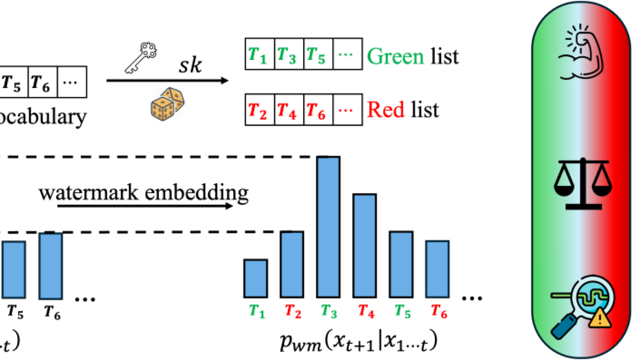


 Robustness. The goal of developing a watermark that is robust to output perturbations is to defend against watermark removal, which may be used to circumvent detection schemes for applications such as phishing or fake news generation. Robust watermark designs have been the topic of many recent works. A more robust watermark can better defend against watermark-removal attacks. However, our work shows that robustness can also enable piggyback spoofing attacks.
 Multiple Keys. Many works have explored the possibility of launching watermark stealing attacks to infer the secret pattern of the watermark, which can then boost the performance of spoofing and removal attacks. A natural and effective defense against watermark stealing is using multiple watermark keys during embedding, which can improve the unbiasedness property of the watermark (it is called distortion-free in the
  Public Detection API. It is still an open question whether watermark detection APIs should be made publicly available to users. Although this makes it easier to detect watermarked text, it is commonly acknowledged that it will make the system vulnerable to attacks. We study this statement more precisely by examining the specific risk trade-offs that exist, as well as introducing a novel defense that may make the public detection API more feasible in practice.