Posted by Khanh LeViet, Developer Advocate on behalf of the TensorFlow Lite team Edge devices, such as smartphones, have become more powerful each year and enable an increasing number of on-device machine learning use cases. TensorFlow Lite is the official framework for running TensorFlow model inference on edge devices. It runs on more than 4 billion active devices globally, on various platforms, including Android, iOS, and Linux-based IoT devices, and on bare metal microcontrollers.
We continue to push the limits of on-device machine learning with TensorFlow Lite by making it faster and easier to use. In this blog post, we highlight recent TensorFlow Lite features that were launched within the past six months, leading up to the TensorFlow Dev Summit in March 2020.
Pushing the limits of on-device machine learning
Enabling state-of-the-art models
Machine learning is a fast-moving field with new models that break the state-of-the-art records every few months. We put a lot of effort into making these state-of-the-art models run well on TensorFlow Lite. As examples, we now support EfficientNet-Lite (paper), a family of image classification models, MobileBERT (paper), and ALBERT-Lite (paper), a light-weight version of BERT (paper) that supports multiple NLP (natural language processing) tasks. Check out some of the performance benchmarks below.
EfficientNet-Lite
EfficientNet-Lite is a family of image classification models that achieve state-of-the-art accuracy with an order of magnitude fewer computations and parameters. The models are optimized for TensorFlow Lite with quantization, resulting in faster inference with negligible accuracy loss, and they can run on the CPU, GPU, or Edge TPU. Find out more in our blog post.
 |
| Figure: Integer-only quantized models running on Pixel 4 CPU with 4 threads. |
MobileBERT and ALBERT-Lite
MobileBERT and ALBERT-Lite are the optimized versions of the popular BERT model that achieved state-of-the-art accuracy on a range of NLP tasks, including question and answer, natural language inference, and others. MobileBERT is about 4x faster and smaller than BERT and retains similar accuracy. Meanwhile, ALBERT-Lite is 6x smaller than BERT, but slower than MobileBERT.
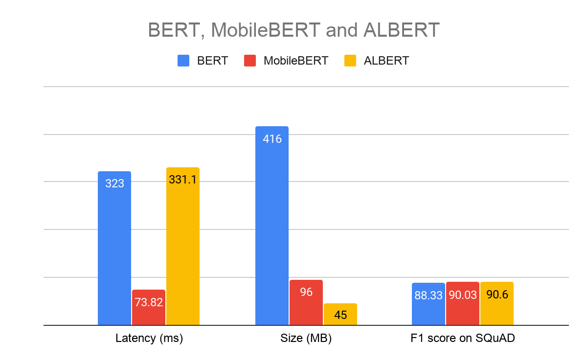 |
| Figure: Pixel 4, Float32 question & answer models, CPU 4 threads |
New TensorFlow Lite converter
We launched a new converter that enables more models and improves the developer experience:
- Enables conversion of new classes of models, including DeepSpeech V2, Mask R-CNN, Mobile BERT, MobileNetSSD, and many more
- Adds support for functional control flow (enabled by default in TensorFlow 2.x)
- Tracks original TensorFlow node names and Python code and exposes them during conversion if errors occur
- Leverages MLIR, Google’s cutting edge compiler technology for ML, which makes it easier to troubleshoot conversion errors and extend to accommodate feature requests
The new converter is fully backward compatible and is enabled by default since TensorFlow 2.2, while the old converter is still available via a flag. See the documentation for more details.
Quantization-aware-training support for Keras
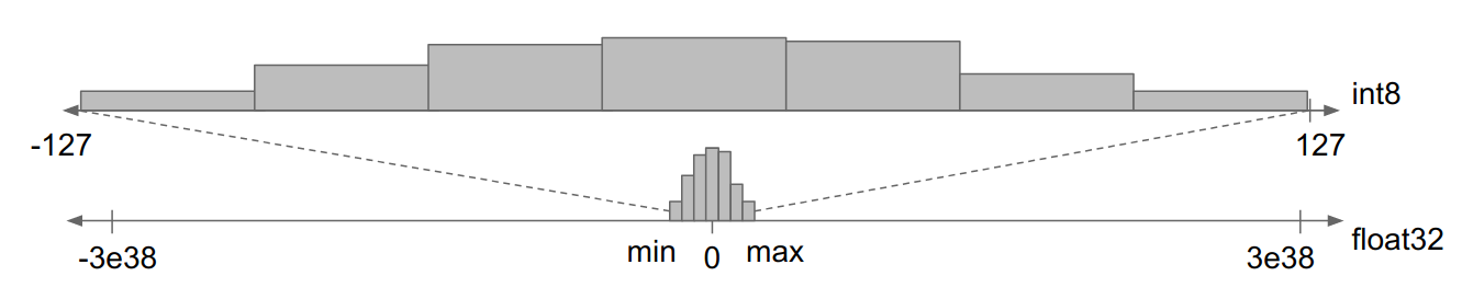
Quantization-aware-training (QAT) enables you to train and deploy models with the performance and size benefits of quantization—makes your model 4x times smaller and run faster, while retaining accuracy. You can add QAT with one line of code.
import tensorflow_model_optimization as tfmot
model = tf.keras.Sequential([
...
])
# Quantize the entire model.
quantized_model = tfmot.quantization.keras.quantize_model(model)
# Continue with training as usual.
quantized_model.compile(...)
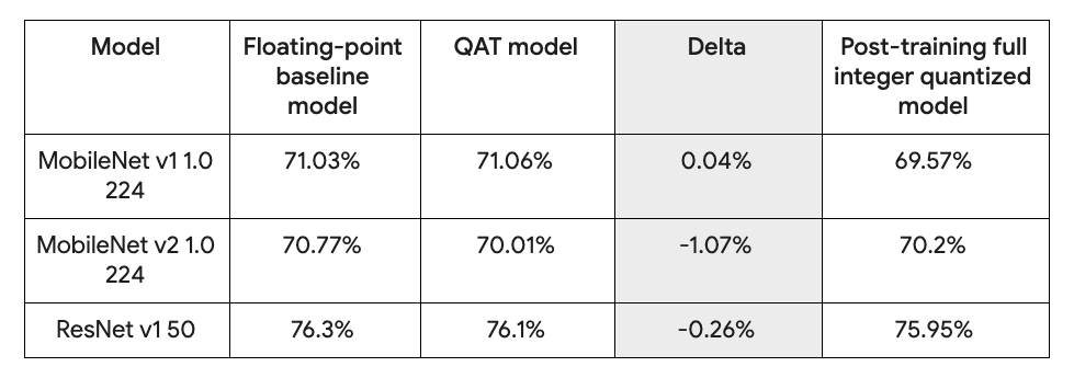
quantized_model.fit(...)Here is how QAT stacks up against the original float model and post-training quantization.  Find out more in our blog post.
Faster inference across platforms
Better CPU performance
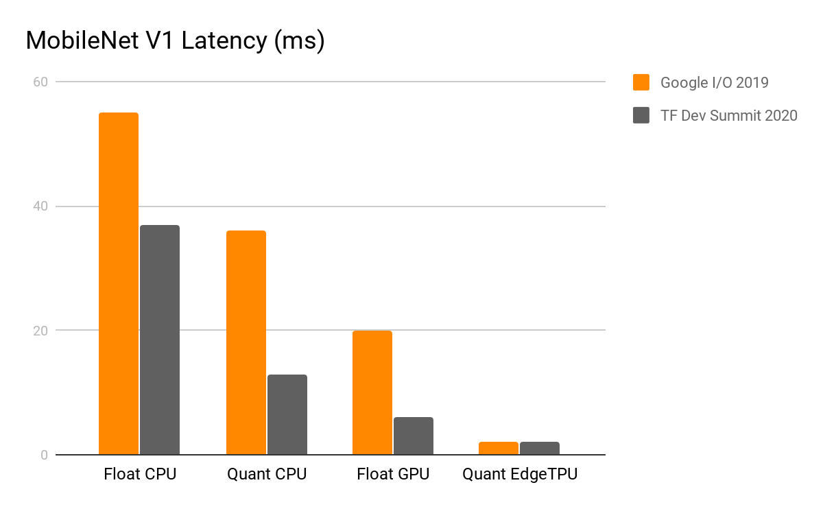
Improving CPU performance has been a major priority for the team and we’ve shipped a number of substantial CPU-related performance optimizations in recent months. As part of this effort, we developed an optimized matrix multiplication library (ruy), built from the ground up to deliver better performance on the classes of CPU hardware and models typically used in mobile environments. As of TensorFlow 1.15, this library is enabled by default for all ARM devices and has helped deliver latency improvements anywhere from 1.2x to 5x across an extremely broad range of models and use cases.
 |
| Pixel 4 – Single Threaded CPU, February 2020 |
We have some additional CPU optimizations scheduled to ship in the TensorFlow 2.3 release, including ~40% faster execution of models with post-training weight quantization, as well as a new highly optimized floating-point convolutional kernel library (XNNPACK) that delivers 20-50% faster execution across all of the key floating-point convolutional models supported by TensorFlow Lite.
Faster inference with new hardware accelerator delegates
TensorFlow Lite is truly cross platform, so that you can train a model once and get the optimal performance on every supported platform. In the past few months, we have added support for running inference on Qualcomm’s Hexagon DSPs, Apple’s Core ML, Android GPU with OpenCL.
Hexagon DSPs are microprocessors that can be found on millions of modern Android phones using Qualcomm Snapdragon SoCs. The new TensorFlow Lite Hexagon delegate leverages the DSP to achieve performance gains in the range of 3-25x for models like MobileNet and Inceptionv3 compared to CPU, while being more power efficient than both CPU and GPU. Learn more in our blog post.
Core ML is the machine learning framework available on Apple’s devices and provides the API to run ML models on Apple’s Neural Engine. The new TensorFlow Lite Core ML delegate allows running TensorFlow Lite models on Core ML and Neural Engine, if available, to achieve faster inference with better power consumption efficiency. On iPhone XS and newer devices, where Neural Engine is available, we have observed performance gains from 1.3x to 11x on various computer vision models. More details can be found in our blog post.
OpenCL is a framework for writing programs that execute across heterogeneous platforms. We recently added support for OpenCL to the TensorFlow Lite GPU delegate, achieving approximately 4-6x speed-up over CPU and approximately 2x speed-up over OpenGL on a variety of computer vision models. Here is a snapshot of the OpenCL backend performance on Pixel 4. 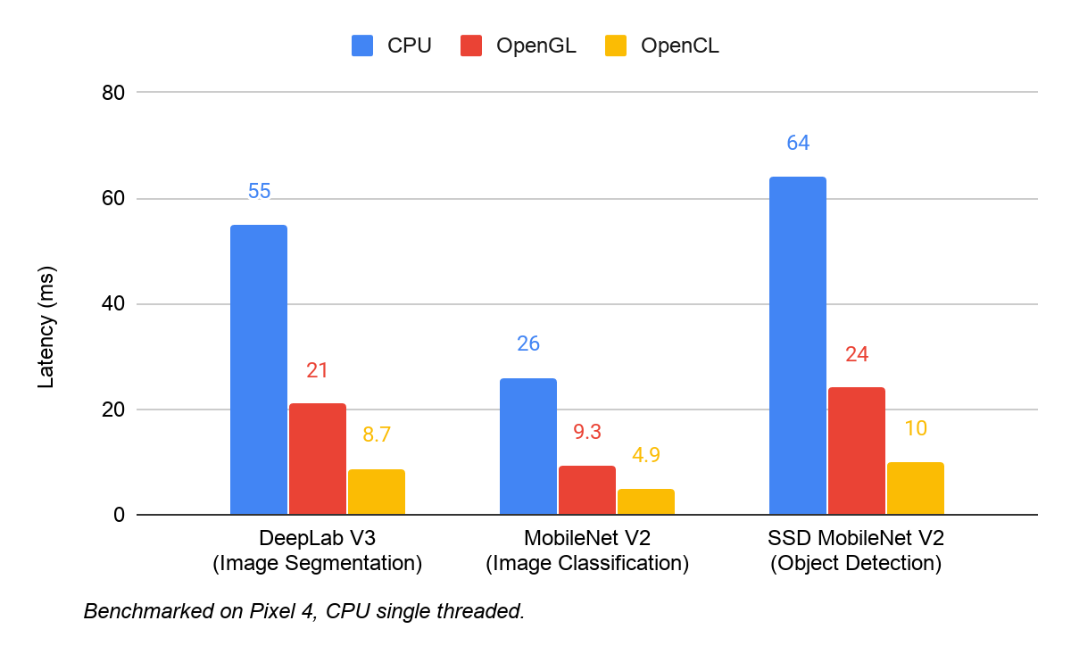
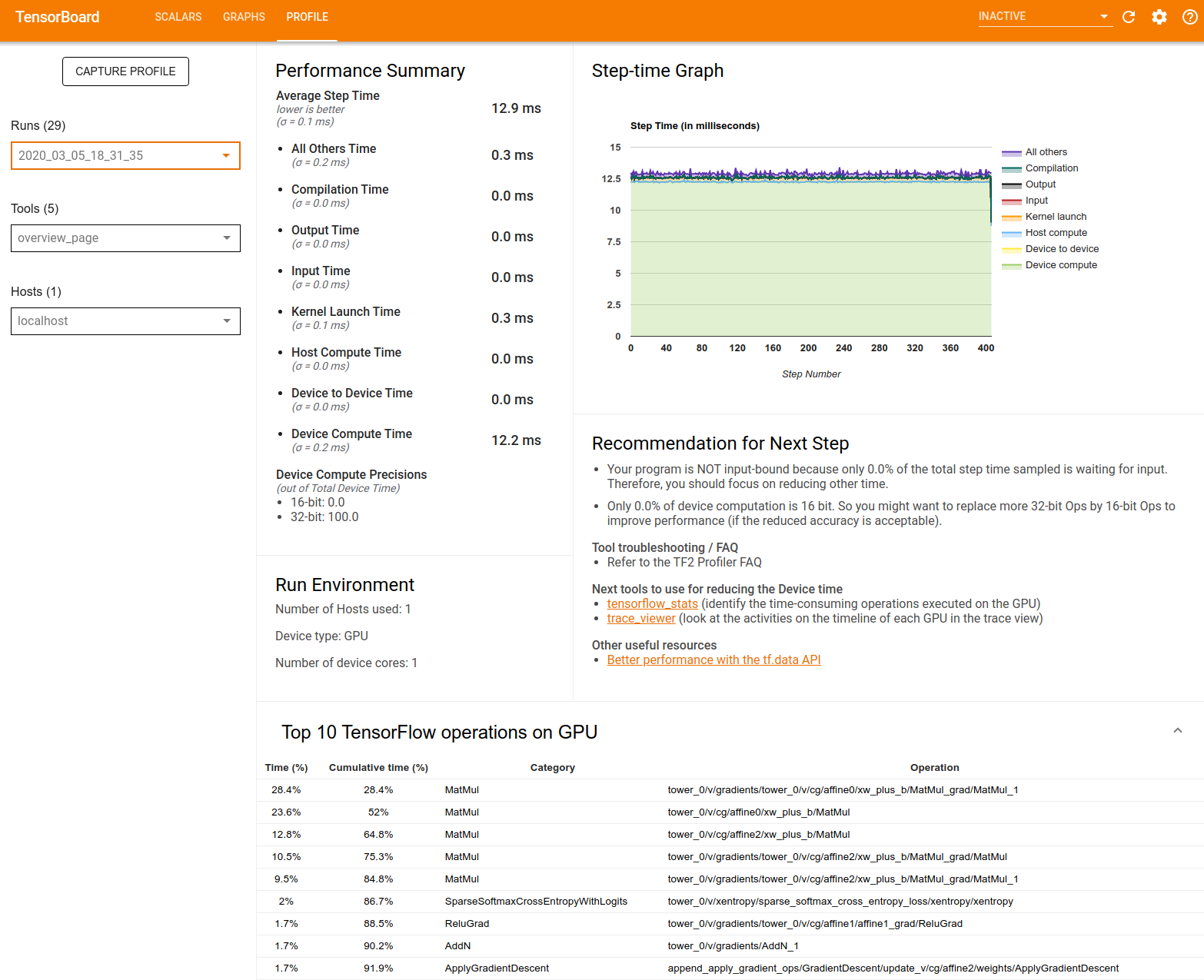
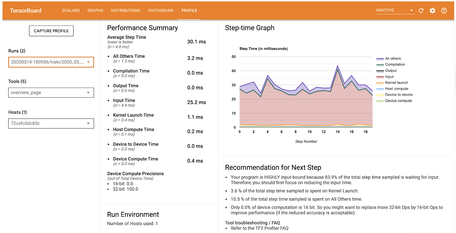
Android performance bottleneck profiler
TensorFlow Lite on Android supports instrumented logging of internal events, including ops invocations, that can be tracked by Android’s system tracing. The new profiling data allows you to identify performance bottlenecks.
Here are some examples of insights that you can get from the profiler and potential solutions to improve performance:
- If the number of available CPU cores is smaller than the number of inference threads, then the CPU scheduling overhead can lead to subpar performance. You can reschedule other CPU intensive tasks in your application to avoid overlapping with your model inference or tweak the number of interpreter threads.
- If the operators are not fully delegated, then some parts of the model graph are executed on the CPU rather than the expected hardware accelerator. You can substitute the unsupported operators with similar supported operators.
This feature is available now in TensorFlow Lite Android library nightly build. More details can be found here. 
Make ML easier to use
Model creation with no ML expertise
TensorFlow Lite Model Maker enables you to adapt state-of-the-art machine learning models to your dataset with transfer learning. It shortens the learning curve for developers new to machine learning by wrapping the complex machine learning concepts with an intuitive API. For example, you can train a state-of-the-art image classification with only four lines of code.
data = ImageClassifierDataLoader.from_folder('flower_photos/')
model = image_classifier.create(data)
loss, accuracy = model.evaluate()
model.export('flower_classifier.tflite', 'flower_label.txt', with_metadata=True)
Model Maker supports many state-of-the-art models that are available on TensorFlow Hub, including the EfficientNet-Lite models mentioned above. It currently supports image classification (tutorial) and text classification (tutorial) with more computer-vision and NLP use cases coming soon.
Model sharing made easy with metadata
Traditionally, running inference with TensorFlow Lite means working with the raw tensors. This presented two hurdles:
- The consumer of the TensorFlow Lite model will need to know exactly what the tensor shape means (e.g. 1 x 224 x 224 x 3). Is it a bitmap? If so, is it in red, blue, and green channels or some other scheme? This poses a problem if the team creating the model is not the same team consuming it.
- The need to use a lot of error-prone boilerplate code to convert from high-level data types, such as
Bitmapto an RGBfloatarray or aByteArray, before it can be used.
To solve the first problem, we added support for model metadata to TensorFlow Lite, allowing model creators to describe the input and output of their model using typed objects. In addition to basic information, such as the size of the bitmap or color channels, we also included information, such as mean and standard deviation, to communicate to the model consumers, so that the appropriate normalization can be applied.
To solve the second problem of boilerplate code, we created the Android code generator, which reads the TensorFlow Lite metadata and creates the appropriate wrapper code to resize, normalize, and convert to and from ByteArray. This means you can now interact with the TensorFlow Lite model using high-level objects that you are familiar with:
// 1. Initializing the Model
MyClassifierModel myImageClassifier = new MyClassifierModel(activity);

// 2. Setting the input with a Bitmap called inputBitmap
MyClassifierModel.Inputs inputs = myImageClassifier.createInputs();
inputs.loadImage(inputBitmap));

// 3. Running the model
MyClassifierModel.Outputs outputs = myImageClassifier.run(inputs);

// 4. Retrieving the result
Map labeledProbability = outputs.getProbability();
This is currently an experimental feature and only supports image-based models. We added metadata support to most TensorFlow Lite vision models on TensorFlow Hub and the Image Classifier Model Maker. Going forward, the project is expanding in three ways:
- Support input types beyond images to enable more use-cases
- Build an Android Studio plugin that makes this even easier to use
- Add iOS support
More sample and learning materials
We launched two online courses on Coursera and Udacity to provide a structured learning path for TensorFlow Lite. Both courses are four weeks long and teach how to use TensorFlow Lite on Android, iOS, and IoT devices.
We released new sample apps demonstrating how to use pretrained models, including style transfer, question and answer and more.  We love to see the engagement in the TensorFlow Lite community. Recently, one member collected pretrained models, samples, and tutorials created by the community and curated them on GitHub. Feel free to contribute!
Better support for microcontrollers
Official support for Arduino
TensorFlow Lite for Microcontrollers is now available as an official Arduino library, which makes it easy to deploy speech detection to an Arduino Nano in under 5 minutes. 
More TensorFlow for Microcontrollers optimizations
We are working with leading industry partners who are writing optimized implementations of TensorFlow Lite for Microcontrollers kernels for their hardware architectures. For example, Cadence announced their support for TensorFlow for Microcontrollers for their Tensilica HiFi DSP family.
How Google is using TensorFlow Lite
TensorFlow Lite is used extensively within Google in many of our key products, including YouTube, Google Assistant, and Google Photos.
The Google Lens team shared how they migrated from a server-based model to a client-based on-device model to improve the user experience.
The Live Perception team showed how to build a machine learning pipeline to process live camera feed in real-time.
What’s next
We have new features and improvements coming in a few months:
- XNNPACK integration for highly optimized floating-point model execution. This will significantly speed up CPU inference across platforms.
- New state-of-the-art on-device models, an updated guide, and examples demonstrating more use cases, such as native C/C++ APIs for inference on mobile.
- Additional tools for trimming binary size based on the ops used in client models, reducing the size impact on client apps.
- Enhancements to Model Maker for more tasks like object detection or NLP tasks. We are adding BERT support to enable new NLP tasks like question and answer, which will empower developers without ML expertise to build state-of-the-art NLP models through transfer learning.
- Expansion of the metadata and codegen tools to support more use cases, including object detection and other NLP-related tasks, and better integration with Android Studio.
To see the longer term TensorFlow Lite product roadmap, please check out our website.Read More