Guest author Hannes Hapke, Senior Data Scientist, SAP Concur Labs. Edited by Robert Crowe on behalf of the TFX team
Transformer models and the concepts of transfer learning in Natural Language Processing have opened up new opportunities around tasks like sentiment analysis, entity extractions, and question-answer problems.
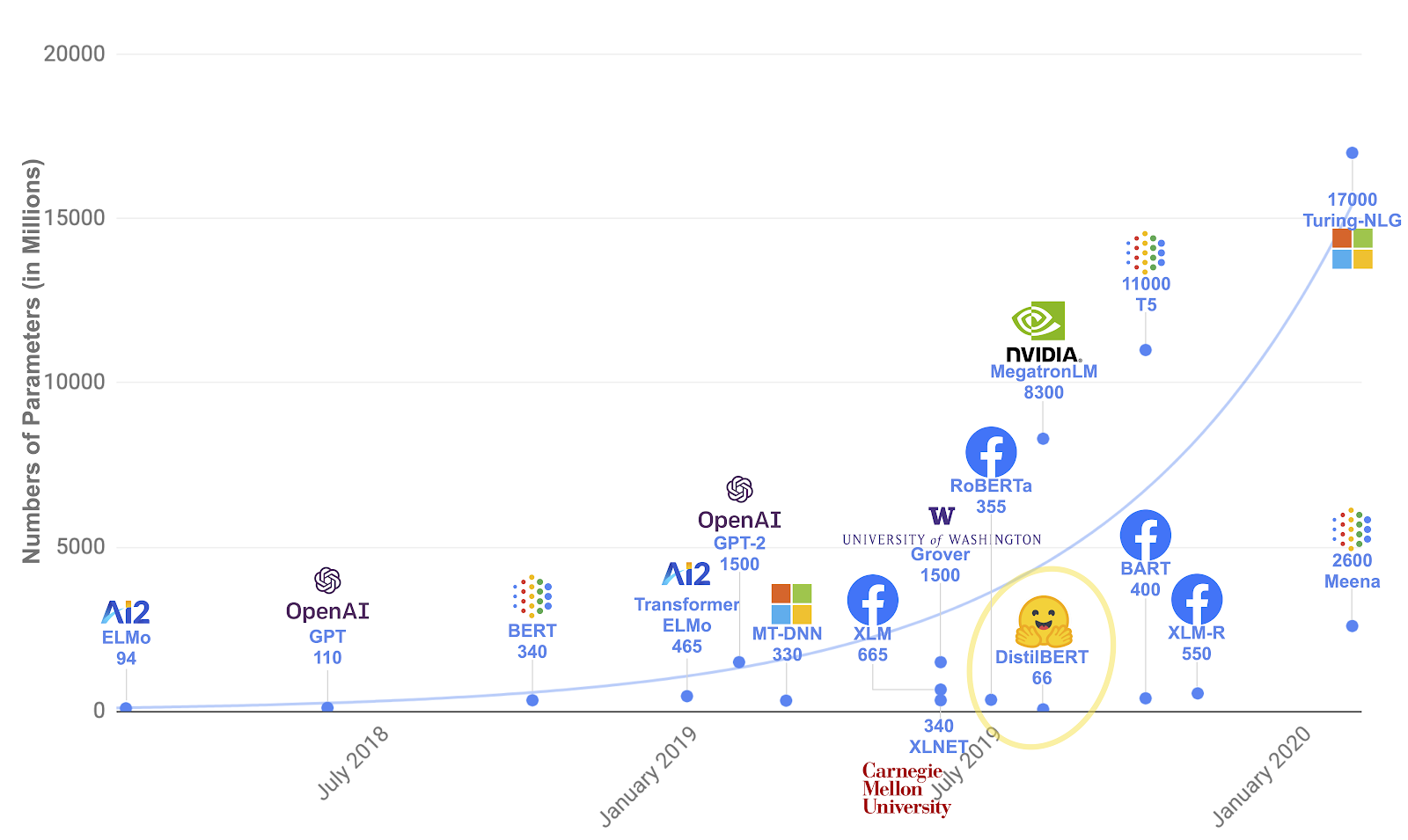
BERT models allow data scientists to stand on the shoulders of giants. Pre-trained on large corpora, data scientists can then apply transfer learning using these multi-purpose trained transformer models and achieve state-of-the-art results for their domain-specific problems.
In part one of our blog post, we discussed why current deployments of BERT models felt too complex and cumbersome and how the deployment can be simplified through libraries and extensions of the TensorFlow ecosystem. If you haven’t checked out the post, we recommend it as a primer for the implementation discussion in this blog post.
At SAP Concur Labs, we looked at simplifying our BERT deployments and we discovered that the TensorFlow ecosystem provides the perfect tools to achieve simple and concise Transformer deployments. In this blog post, we want to take you on a deep dive of our implementation and how we use components of the TensorFlow ecosystem to achieve scalable, efficient and fast BERT deployments.
Want to jump ahead to the code?
If you would like to jump to the complete example, check out the Colab notebook. It showcases the entire TensorFlow Extended (TFX) pipeline we used to produce a deployable BERT model with the preprocessing steps as part of the model graph. If you want to try out our demo deployment, check out our demo page at SAP ConcurLabs showcasing our sentiment classification project.
Why use Tensorflow Transform for Preprocessing?
Before we answer this question, let’s take a quick look at how a BERT transformer works and how BERT is currently deployed.
What preprocessing does BERT require?
Transformers like BERT are initially trained with two main tasks in mind: masked language models and next sentence predictions (NSP). These tasks require an input data structure beyond the raw input text. Therefore, the BERT model requires, besides the tokenized input text, a tensor input_type_ids to distinguish between different sentences. A second tensor input_mask is used to note the relevant tokens within the input_word_ids tensor. This is required because we will expand our input_word_ids tensors with pad tokens to reach the maximum sequence length. That way all input_word_ids tensors will have the same lengths but the transformer can distinguish between relevant tokens (tokens from our input sentence) and irrelevant pads (filler tokens).
 |
| Figure 1: BERT tokenization |
Currently, with most transformer model deployments, the tokenization and the conversion of the input text is either handled on the client side or on the server side as part of a pre-processing step outside of the actual model prediction.
This brings a few complexities with it: if the preprocessing happens on the client side then all clients need to be updated if the mapping between tokens and ids changes (e.g., when we want to add a new token). Most deployments with server-side preprocessing use a Flask-based web application to accept the client requests for model predictions, tokenize and convert the input sentence, and then submit the data structures to the deep learning model. Having to maintain two “systems” (one for the preprocessing and one for the actual model inference) is not just cumbersome and error prone, but also makes it difficult to scale.
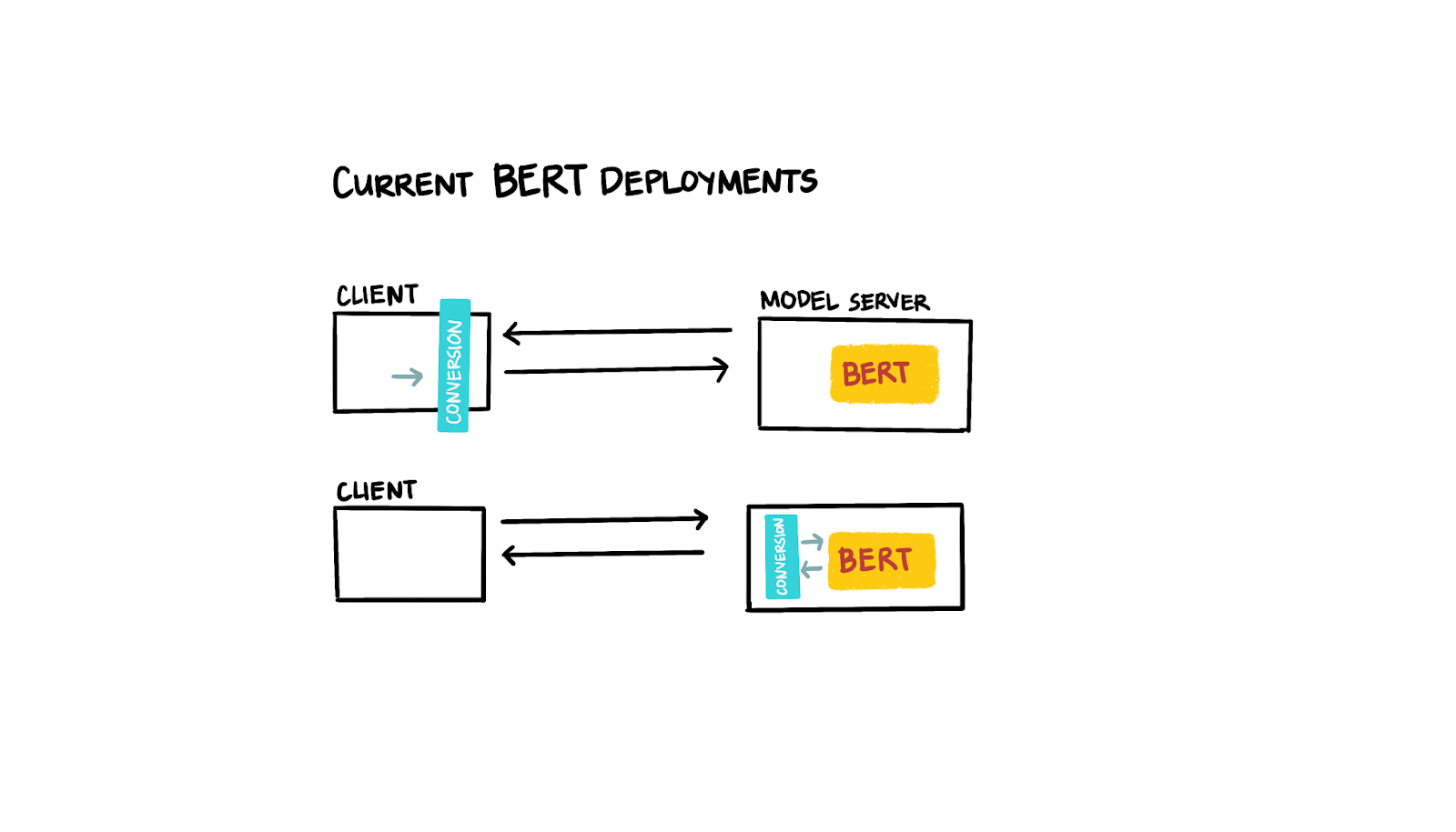 |
| Figure 2: Current BERT deployments |
It would be great if we could get the best of both solutions: easy scalability and simple upgradeability. With TensorFlow Transform (TFT), we can achieve both requirements by building the preprocessing steps as a graph, exporting them together with the deep learning model, and ultimately only deploying one “system” (our combined deep learning model with the integrated preprocessing functionality). It’s worth pointing out that moving all of BERT into preprocessing is not an option when we want to fine-tune the tf.hub module of BERT for our domain-specific task.
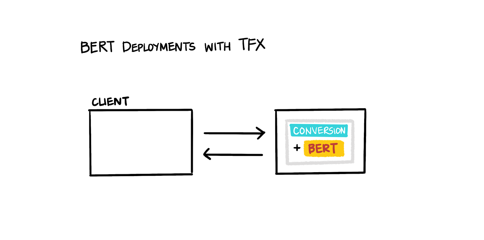 |
| Figure 3: BERT with TFX |
Processing Natural Language with tf.text
In 2019, the TensorFlow team released a new tensor type: RaggedTensors which allow storing arrays of different lengths in a tensor. The implementation of RaggedTensors became very useful specifically in NLP applications, e.g., when we want to tokenize a 1-D array of sentences into a 2-D RaggedTensor with different array lengths.
Before tokenization:
[
 “Clara is playing the piano.”
 “Maria likes to play soccer.’”
 “Hi Tom!”
]
After the tokenization:
[
   [[b'clara'], [b'is'], [b'playing'], [b'the'], [b'piano'], [b'.']],
   [[b'maria'], [b'likes'], [b'to'], [b'play'], [b'soccer'], [b'.']],
   [[b'hi'], [b'tom'], [b'!']]
]
As we will see in a bit, we use RaggedTensors for our preprocessing pipelines. In late October 2019, the TensorFlow team then released an update to the tf.text module which allows wordpiece tokenization required for the preprocessing of BERT model inputs.
import tensorflow_text as text

vocab_file_path = bert_layer.resolved_object.vocab_file.asset_path.numpy()
do_lower_case = bert_layer.resolved_object.do_lower_case.numpy()

bert_tokenizer = text.BertTokenizer(
vocab_lookup_table=vocab_file_path,
token_out_type=tf.int64,
lower_case=do_lower_case)
TFText provides a comprehensive tokenizer specific for the wordpiece tokenization (BertTokenizer) required by the BERT model. The tokenizer provides the tokenization results as strings (tf.string) or already converted to word_ids (tf.int32).
NOTE: The tf.text version needs to match the imported TensorFlow version. If you use TensorFlow 2.2.x, you will need to install TensorFlow Text version 2.2.x, not 2.1.x or 2.0.x.
How can we preprocess text with TensorFlow Transform?
Earlier, we discussed that we need to convert any input text to our Transformer model into the required data structure of input_word_ids, input_mask, and input_type_ids. We can perform the conversion with TensorFlow Transform. Let’s have a closer look.
For our example model, we want to classify the sentiment of IMDB reviews using the BERT model.
    ‘This is the best movie I have ever seen ...’       -> 1
 ‘Probably the worst movie produced in 2019 ...’     -> 0
 ‘Tom Hank’s performance turns this movie into ...’ -> ?
That means that we’ll input only one sentence with every prediction. In practice, that means that all submitted tokens are relevant for the prediction (noted by a vector of ones) and all tokens are part of sentence A (noted by a vector of zeros). We won’t submit any sentence B in our classification case.
If you want to use a BERT model for other tasks, e.g., predicting the similarity of two sentences, entity extraction or question-answer tasks, you would have to adjust the preprocessing step.
Since we want to export the preprocessing steps as a graph, we need to use TensorFlow ops for all preprocessing steps exclusively. Due to this requirement, we can’t reuse functions of Python’s standard library which are implemented in CPython.
The BertTokenizer, provided by TFText, handles the preprocessing of the incoming raw text data. There is no need for lower casing your strings (if you use the uncased BERT model) or removing unsupported characters. The tokenizer from the TFText library requires a table of the support tokens as input. The tokens can be provided as TensorFlow LookupTable, or simply as a file path to a vocabulary file. The BERT model from TFHub provides such a file and we can determine the file path with
import tensorflow_hub as hub

BERT_TFHUB_URL = "https://tfhub.dev/tensorflow/bert_en_uncased_L-12_H-768_A-12/2"
bert_layer = hub.KerasLayer(handle=BERT_TFHUB_URL, trainable=True)
vocab_file_path =
    bert_layer.resolved_object.vocab_file.asset_path.numpy()
Similarly, we can determine if the loaded BERT model is case-sensitive or not.
do_lower_case = bert_layer.resolved_object.do_lower_case.numpy()
We can now pass the two arguments to our TFText BertTokenizer and specify the data type of our tokens. Since we are passing the tokenized string to the BERT model, we need to provide the tokens as token indices (provided as int64 integers)
bert_tokenizer = text.BertTokenizer(
vocab_lookup_table=vocab_file_path,
token_out_type=tf.int64,
lower_case=do_lower_case
)
After instantiating the BertTokenizer, we can perform the tokenizations with the tokenize method.
tokens = bert_tokenizer.tokenize(text)
Once the sentence is tokenized into token ids, we will need to prepend the start and append a separation token.
 CLS_ID = tf.constant(101, dtype=tf.int64)
    SEP_ID = tf.constant(102, dtype=tf.int64)
    start_tokens = tf.fill([tf.shape(text)[0], 1], CLS_ID)
    end_tokens = tf.fill([tf.shape(text)[0], 1], SEP_ID)
    tokens = tokens[:, :sequence_length - 2]
    tokens = tf.concat([start_tokens, tokens, end_tokens], axis=1)
At this point, our token tensors are still ragged tensors with different lengths. TensorFlow Transform expects all tensors to have the same length, therefore we will be padding the truncating the tensors to a maximum length (MAX_SEQ_LEN) and pad shorter tensors with a defined pad token.
PAD_ID = tf.constant(0, dtype=tf.int64)
tokens = tokens.to_tensor(default_value=PAD_ID)
      padding = sequence_length - tf.shape(tokens)[1]
      tokens = tf.pad(tokens,
     [[0, 0], [0, padding]],
     constant_values=PAD_ID)
The last step provides us with constant length token vectors which are the final step of the major preprocessing steps. Based on the token vectors, we can create the two required, additional data structures, input_mask, and input_type_ids.
In the case of the input_mask, we want to note all relevant tokens, basically all tokens besides the pad token. Since the pad token has the value zero and all ids are greater or equal zero, we can define the input_mask with the following ops.
input_word_ids = tokenize_text(text)
        input_mask = tf.cast(input_word_ids > 0, tf.int64)
        input_mask = tf.reshape(input_mask, [-1, MAX_SEQ_LEN])
To determine the input_type_ids is even simpler in our case. Since we are only submitting one sentence, the type ids are all zero in our classification example.
input_type_ids = tf.zeros_like(input_mask)
To complete the preprocessing setup, we will wrap all steps in the preprocessing_fn function which is required by TensorFlow Transform.
def preprocessing_fn(inputs):

    def tokenize_text(text, sequence_length=MAX_SEQ_LEN):
   ...
        return tf.reshape(tokens, [-1, sequence_length])

    def preprocess_bert_input(text, segment_id=0):
        input_word_ids = tokenize_text(text)
        ...
        return (
            input_word_ids,
            input_mask,
            input_type_ids
        )
    ...

    input_word_ids, input_mask, input_type_ids =
        preprocess_bert_input(_fill_in_missing(inputs['text']))

    return {
        'input_word_ids': input_word_ids,
        'input_mask': input_mask,
        'input_type_ids': input_type_ids,
        'label': inputs['label']
    }
Train the Classification Model
The latest updates of TFX allow the use of native Keras models. In the example code below, we define our classification model. The model takes advantage of the pretrained BERT model and KerasLayer provided by TFHub. To avoid any misalignment between the transform step and the model training, we are creating the input layers dynamically based on the feature specification provided by the transformation step.
 feature_spec = tf_transform_output.transformed_feature_spec()
    feature_spec.pop(_LABEL_KEY)

    inputs = {
key: tf.keras.layers.Input(
shape=(max_seq_length),
name=key,
dtype=tf.int32)
            for key in feature_spec.keys()}
We need to cast the variables since TensorFlow Transform can only output variables as one of the types: tf.string, tf.int64 or tf.float32 (tf.int64 in our case). However, the BERT model from TensorFlow Hub used in our Keras model above expects tf.int32 inputs. So, in order to align the two TensorFlow components, we need to cast the inputs in the input functions or in the model graph before passing them to the instantiated BERT layer.
 input_word_ids = tf.cast(inputs["input_word_ids"], dtype=tf.int32)
    input_mask = tf.cast(inputs["input_mask"], dtype=tf.int32)
    input_type_ids = tf.cast(inputs["input_type_ids"], dtype=tf.int32)
Once our inputs are converted to tf.int32 data types, we can pass them to our BERT layer. The layer returns two data structures: a pooled output, which represents the context vector for the entire text and list of vectors providing context specific vector representation for each submitted token. Since we are only interested in the classification of the entire text, we can ignore the second data structure.
bert_layer = load_bert_layer()
    pooled_output, _ = bert_layer(
        [input_word_ids,
         input_mask,
         input_type_ids
        ]
    )
Afterwards, we can assemble our classification model with tf.keras. In our example, we used the functional Keras API.
 x = tf.keras.layers.Dense(256, activation='relu')(pooled_output)
    dense = tf.keras.layers.Dense(64, activation='relu')(x)
    pred = tf.keras.layers.Dense(1, activation='sigmoid')(dense)

    model = tf.keras.Model(
        inputs=[inputs['input_word_ids'],
                inputs['input_mask'],
                inputs['input_type_ids']],
        outputs=pred
    )
    model.compile(loss='binary_crossentropy',
                  optimizer='adam',
                  metrics=['accuracy'])
The Keras model can then be consumed by our run_fn function which is called by the TFX Trainer component. With the recent updates to TFX, the integration of Keras models was simplified. No “detour” with TensorFlow’s model_to_estimator function is required anymore. We can now define a generic run_fn function which executes the model training and exports the model after the completion of the training.
Here is an example of the setup of a run_fn function to work with the latest TFX version:
def run_fn(fn_args: TrainerFnArgs):
    tf_transform_output = tft.TFTransformOutput(fn_args.transform_output)
    train_dataset = _input_fn(
        fn_args.train_files, tf_transform_output, 32)
    eval_dataset = _input_fn(
        fn_args.eval_files, tf_transform_output, 32)

    mirrored_strategy = tf.distribute.MirroredStrategy()
    with mirrored_strategy.scope():
        model = get_model(tf_transform_output=tf_transform_output)

    model.fit(
        train_dataset,
        steps_per_epoch=fn_args.train_steps,
        validation_data=eval_dataset,
        validation_steps=fn_args.eval_steps)

    signatures = {
        'serving_default':
            _get_serve_tf_examples_fn(model, tf_transform_output
            ).get_concrete_function(
                                 tf.TensorSpec(
                                 shape=[None],
                                 dtype=tf.string,
                                 name='examples')),
    }
    model.save(
        fn_args.serving_model_dir,
        save_format='tf',
        signatures=signatures)
It is worth taking special note of a few lines from the example Trainer function. With the latest release of TFX, we can now take advantage of the distribution strategies introduced in Keras last year in our TFX trainer components.
mirrored_strategy = tf.distribute.MirroredStrategy()
    with mirrored_strategy.scope():
        model = get_model(tf_transform_output=tf_transform_output)
It is most efficient to preprocess the data sets ahead of the model training, which allows for faster training, especially when the trainer passes multiple times over the same data set.
Therefore, TensorFlow Transform will perform the preprocessing prior to the training and evaluation, and store the preprocessed data as TFRecords.
{'input_mask': array([1, 1, 1, 1, 1, 1, 1, 1, 1, 1, 1, 1, 1, 1, 1, 1, 1, 1, 1, 1, 1, 1]),
 'input_type_ids': array([0, 0, 0, 0, 0, 0, 0, 0, 0, 0, 0, 0, 0, 0, 0, 0, 0, 0, 0, 0, 0, 0]),
 'input_word_ids': array([  101,  2023,  3319,  3397, 27594,  2545,  2005,  2216,  2040, ..., 2014,   102]),
 'label': array([0], dtype=float32)}
This allows us to generate a preprocessing graph which then can be applied during our post-training prediction mode. Because we reuse the preprocessing graph, we can avoid skew between the training and the prediction preprocessing.
In our run_fn function we can then “wire up” the preprocessed training and evaluation data sets instead of the raw data sets to be used during the training:
 tf_transform_output = tft.TFTransformOutput(fn_args.transform_output)
    train_dataset = _input_fn(fn_args.train_files, tf_transform_output, 32)
    eval_dataset = _input_fn(fn_args.eval_files, tf_transform_output, 32)
         ...
    model.fit(
        train_dataset,
        validation_data=eval_dataset,
        ...)
Once the training is completed, we can export our trained model together with the processing steps.
Export the Model with its Preprocessing Graph
After the model.fit() completes the model training, we are calling model.save()to export the model in the SavedModel format. In our model signature definition, we are calling the function _get_serve_tf_examples_fn() which parses serialized tf.Example records submitted to our TensorFlow Serving endpoint (e.g. in our case the raw text strings to be classified) and then applies the transformations preserved in the TensorFlow Transform graph. The model prediction is then performed with the transformed features which are the output of the model.tft_layer(parsed_features)call. In our case, this would be the BERT token ids, masks ids and type ids.
def _get_serve_tf_examples_fn(model, tf_transform_output):
   model.tft_layer = tf_transform_output.transform_features_layer()

   @tf.function
   def serve_tf_examples_fn(serialized_tf_examples):
       feature_spec = tf_transform_output.raw_feature_spec()
       feature_spec.pop(_LABEL_KEY)
       parsed_features = tf.io.parse_example(serialized_tf_examples, feature_spec)

       transformed_features = model.tft_layer(parsed_features)
       return model(transformed_features)

   return serve_tf_examples_fn
The _get_serve_tf_examples_fn() function is the important connection between the transformation graph generated by TensorFlow Transform, and the trained tf.Keras model. Since the prediction input is passed through the model.tft_layer(), it guarantees that the exported SavedModel will include the same preprocessing that was performed during training. The SavedModel is one graph, consisting of both the preprocessing and the model graphs.
With the deployment of the BERT classification model through TensorFlow Serving, we can now submit raw strings to our model server (submitted as tf.Example records) and receive a prediction result without any preprocessing on the client side or a complicated model deployment with a preprocessing step.
Future work
The presented work allows a simplified deployment of BERT models. The preprocessing steps shown in our demo project can easily be extended to handle more complicated preprocessing, e.g., for tasks like entity extractions or question-answer tasks. We are also investigating if the prediction latency can be further reduced if we reuse a quantized or distilled version of the pre-trained BERT model (e.g., Albert).
Thank you for reading our two-part blog post. Feel free to get in touch if you have questions or recommendations by email.
Further Reading
If you are interested in an overview of the TensorFlow libraries we used in this project, we recommend the part one of this blog post.
In case you want to try out our demo deployment, check out our demo page at SAP ConcurLabs showcasing our sentiment classification project.
If you are interested in the inner workings of TensorFlow Extended (TFX) and TensorFlow Transform, check out this upcoming O’Reilly publication “Building Machine Learning Pipelines with TensorFlow” (pre-release available online).
For more information
To learn more about TFX check out the TFX website, join the TFX discussion group, dive into other posts in the TFX blog, watch our TFX playlist on YouTube, and subscribe to the TensorFlow channel.
Acknowledgments
This project wouldn’t have been possible without the tremendous support from Catherine Nelson, Richard Puckett, Jessica Park, Robert Reed, and the SAP’s Concur Labs team. Thanks goes also out to Robert Crowe, Irene Giannoumis, Robby Neale, Konstantinos Katsiapis, Arno Eigenwillig, and the rest of the TensorFlow team for discussing implementation details and for the detailed review of this post. A special thanks to Varshaa Naganathan, Zohar Yahav, and Terry Huang from Google’s TensorFlow team for providing updates to the TensorFlow libraries to make this pipeline implementation possible. Big thanks also to Cole Howard from Talenpair for always enlightening discussions about Natural Language Processing.
Read More


 As we can see, for some predictions (especially where no singing voice is present), the confidence is very low. Let’s only keep the predictions with high confidence by removing the results where the confidence was below 0.9.
 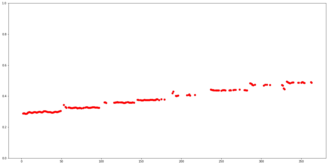 To confirm that the model is working correctly, let’s convert pitch from the [0.0, 1.0] range to absolute values in Hz. To do this conversion we can use the function present in the Colab notebook:
 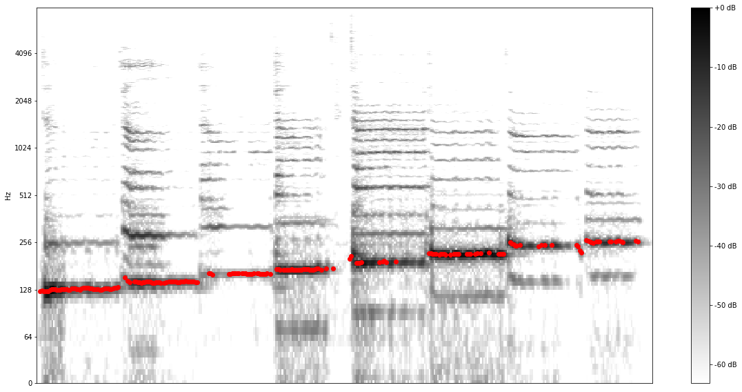 Success! We managed to extract the relevant pitch from the singer’s voice.
  We can also export the converted notes to a MIDI file using music21:


