Posts in category: Tensorflow

Posted by Jocelyn Becker, Program Manager, TensorFlow Certificate
Four months ago at the 2020 TensorFlow Dev Summit, we launched the TensorFlow Developer Certificate to provide everyone in the world the opportunity to showcase their expertise in ML in an increasingly AI-driven global job market.

Today is a big milestone for our community because 500 people from around the world have officially passed the exam! This group of certificate holders spans 6 continents and 55 countries. You can see those who have joined our credential network here.

We are excited to see the benefits of the certificate come to life. For example, Iago González Basadre, on the Business Development team for Premium Leads in Spain, took the exam to help him prepare for hiring a dedicated team to work on AI at his company. He said, “This exam was a great help to me. During this COVID pandemic, I’ve spent a lot of time at home, and I could work a lot with TensorFlow to create models and improve our products by myself.”

Also, since launching, to ensure the exam is accessible, we are proud to have awarded over 200 stipends to ML practitioners. We are eager to scale this program by adding certificate programs for more advanced and specialized TensorFlow practitioners in the future.

Interested in taking the exam? This certificate in TensorFlow development is intended as a foundational certificate for students, developers, and data scientists who want to demonstrate practical machine learning skills through the building and training of models using TensorFlow. Jeffrey Luppes, a machine learning engineer for Atos, in Amsterdam says, “the exam creates a real-world testing environment, rather than a typical proctored exam with somebody looking over your shoulder. You can multitask and use Stack Overflow, which simulates development in the real world.”

Learn more about the TensorFlow Developer Certificate on our website, including information on exam criteria, exam cost, and a stipend to make this more accessible.

Congratulations to those who have passed, and we look forward to growing this community of TensorFlow Developer Certificate recipients!
Read More

Posted by Pohung Chen, Creative Technologist, Google Partner Innovation

Today we are releasing LipSync, a web experience that lets you lip sync to music live in the web browser. LipSync was created as a playful way to demonstrate the facemesh model for TensorFlow.js. We partnered with Australian singer Tones and I to let you lip sync to Dance Monkey in this demonstration.

Using TensorFlow.js FaceMesh

The TensorFlow.js FaceMesh model provides a real-time high density estimate of key points of your facial expression using only a webcam and on device machine learning – meaning no data ever leaves your machine for inference. We essentially use the key points around the mouth and lips to estimate how well you synchronize to the lyrics of the Dance Monkey song.

Determining Correctness

When first testing the demo, many people assumed we used a complex lip reading algorithm to match the mouth shapes with lyrics. Lip reading is quite difficult to achieve, so we came up with a simpler solution. We capture a frame by frame recording of the “correct” mouth shapes lined up with the music, and then when the user is playing the game, we compare the mouth shapes to the pre-recorded baseline.

Measuring the shape of your mouth

What is a mouth shape? There are many different ways to measure the shape of your mouth. We needed a technique that allows the user to move their head around while singing and is relatively forgiving in different mouth shapes, sizes, and distance to the camera.

Mouth Ratio

One way of comparing mouth shapes is to use the width to height ratio of your mouth. For example, if your mouth is closed and forming the “mmm” sound, you have a high width to height ratio. If your mouth is open in an “ooo” sound, your mouth will be closer to a 1:1 width to height ratio.
While this method mostly works, there were still edge cases that made the detection algorithm not as robust, so we explored another method called Hu Moments explained below.

OpenCV matchShapes Hu Moments

In the OpenCV library, there is a matchShapes function which compares contours and returns a similarity score. Underneath the hood, the matchShapes function uses a technique called Hu Moments which provides a set of numbers calculated using central moments that are invariant to image transformations. This allowed us to compare shapes regardless of translation, scale, and rotation. So the user can freely rotate their head without impacting the detection of the mouth shape itself.

We use this in addition to the mouth shape above to determine how closely the shape of the mouth contours match.

Visual and Audio Feedback

In our original prototype, we wanted to create immediate audible feedback on how well the user is doing. We separated out the vocal track from the rest of the song and changed its volume based on real-time user performance score of their mouth shapes.

Vocal Track

Instrumental Track

This allowed us to create the effect such that if you stop lip syncing to the song, the lyrical portion of the song stops playing (but the background music continues to play).

While this was a fun way to demonstrate the mouth shape matching algorithm, however it still missed that satisfactory rush of joy you get when you hit the right notes during karaoke or nail a long sequence of moves just right in arcade rhythm games.

We started by adding a real-time score that is then accumulated over time shown to the player as they played the game. In our initial testing, this didn’t work as well as we had hoped. It was confusing what the score was and the exact numbers weren’t particularly meaningful. We also wanted the user to focus their attention on the lyrics and the center of the screen as opposed to a score off to the side.

So we went with a different approach, preferring to lean on visual effects overlaid on top of the player’s face as they lip synced to the music and colors to indicate how well the player was doing.

Try Lip Sync yourself!

The Tensorflow.js FaceMesh model enables web-based, playful, interactive experiences that go beyond basic face filters, and with a little bit of creative thinking, we could get a lip sync experience without needing the full complexity of a full lip reading ML model.

So go ahead and try our live demo yourself right now. You can also check out an example of how the mouth shape matching works in this open source repo.

We would also like to give a special shout out to Kiattiyot Panichprecha, Bryan Tanaka, KC Chung, Dave Bowman, Matty Burton, Roger Chang, Ann Yuan, Sandeep Gupta, Miguel de Andrés-Clavera, Alessandra Donati, and Ethan Converse for their help in bringing this experience to life, and to thank the MediaPipe team who designed Facemesh.Read More

Posted by Miguel de Andrés-Clavera, Product Manager, Google PI

In this post, I’d like to share with you a demo we built for (and had planned to show at) Google I/O this year with TensorFlow Lite. I wish we had the opportunity to meet in person, but I hope you find this article interesting nonetheless!

Pixelopolis

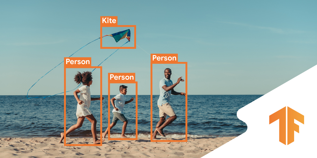
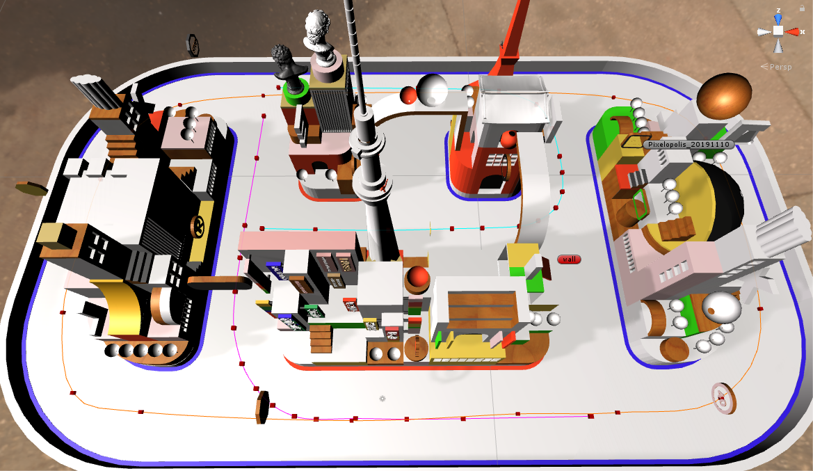
Pixelopolis is an interactive installation that showcases self-driving miniature cars powered by TensorFlow Lite. Each car is outfitted with its own Pixel phone, which used its camera to detect and understand signals from the world around it. In order to sense lanes, avoid collisions and read traffic signs, the phone uses machine learning running on the Pixel Neural Core, which contains a version of an Edge TPU.

An edge computing implementation is a good option to make projects like this possible. Processing video and detecting objects are much more difficult using Cloud-based methods – due to latency. If you can, doing it on-device is much faster.

Users can interact with Pixelopolis via a “station” (an app running on a phone), where they can select the destination the car will drive to. The car will navigate to the destination, and during the journey, the app shows real-time streaming video from the Car — this allows the user to see what the car sees and detects. As you may notice from the gifs below, Pixelopolis has multilingual support built-in as well.

Station App

Car App

How it works

Using the front camera on a mobile device, we perform lane-keeping, localization and object detection right on the device in real-time. Not only that, in our case, the Pixel 4 also controls the motors and other electronic components via USB-C, so the car can stop when it detects other cars or turn at a right interaction when it needs to.

If you’re interested in technical details, the remainder of this article describes the major components of the car, and our journey building it.

Lane-keeping

We explored a variety of models for Lane-keeping. As a baseline, we used a CNN to detect the traffic lines in each frame and adjust the steering wheel every frame, which works fine. We improved this by adding an LSTM and using multiple previous frames. After experimenting a bit more, we followed a similar model architecture to this paper.

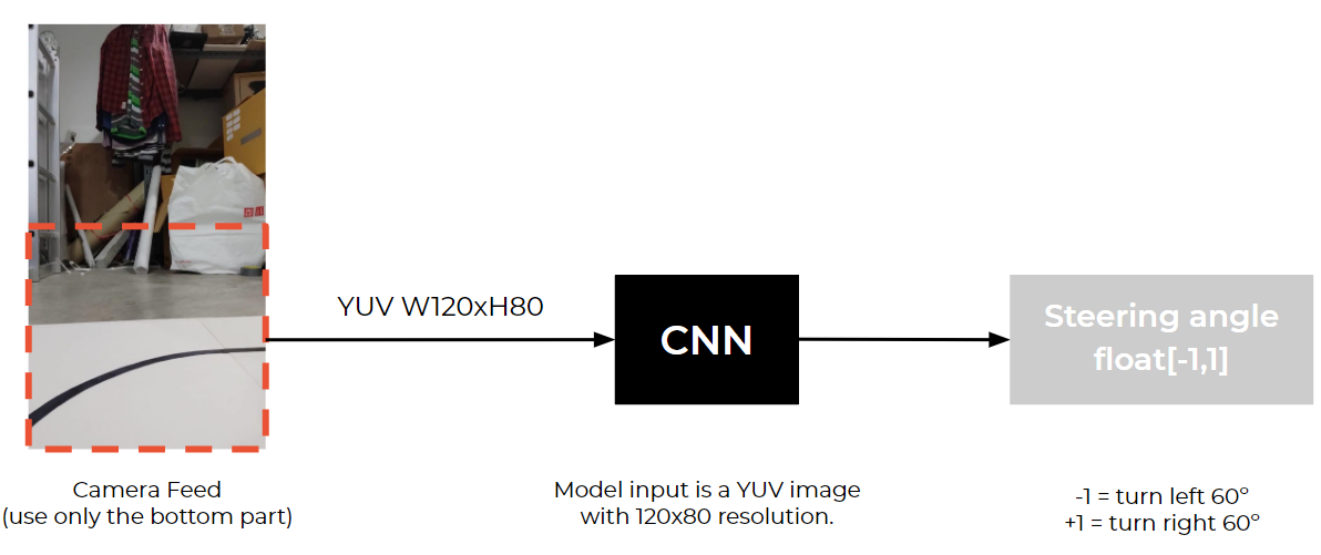CNN model input and output

Model Architecture

net_in = Input(shape = (80, 120, 3))
x = Lambda(lambda x: x/127.5 - 1.0)(net_in)
x = Conv2D(24, (5, 5), strides=(2, 2),padding="same", activation='elu')(x)  
x = Conv2D(36, (5, 5), strides=(2, 2),padding="same", activation='elu')(x)
x = Conv2D(48, (5, 5), strides=(2, 2),padding="same", activation='elu')(x)
x = Conv2D(64, (3, 3), padding="same",activation='elu')(x)   
x = Conv2D(64, (3, 3), padding="same",activation='elu')(x)
x = Dropout(0.3)(x)
x = Flatten()(x)
x = Dense(100, activation='elu')(x)
x = Dense(50, activation='elu')(x)
x = Dense(10, activation='elu')(x) 
net_out = Dense(1, name='net_out')(x)
model = Model(inputs=net_in, outputs=net_out)

Data Collection

Before we are able to use this model, we need to find a way to collect the image data from the car to train. The problem is we didn’t have a car or a track to use at the time. So, we decided to use a simulator. We chose Unity and this simulator project from Udacity for lane-keeping data collection.

Multiple waypoints on the track in the simulator

By setting multiple waypoints on the track, the car bot is able to drive to different locations and also collects data for us. In this simulator, we collect image data and steering angle every 50ms.

Image Augmentation

Data Augmentation with various environments

Since we do all data collection within the simulator, we need to create various environments in the scene because we want our model to be able to handle different lighting, background environment and other noises. We added these variables to the scene: random HDRI sphere ( with different rotation and exposure values), random brightness and color, and random cars.

Training

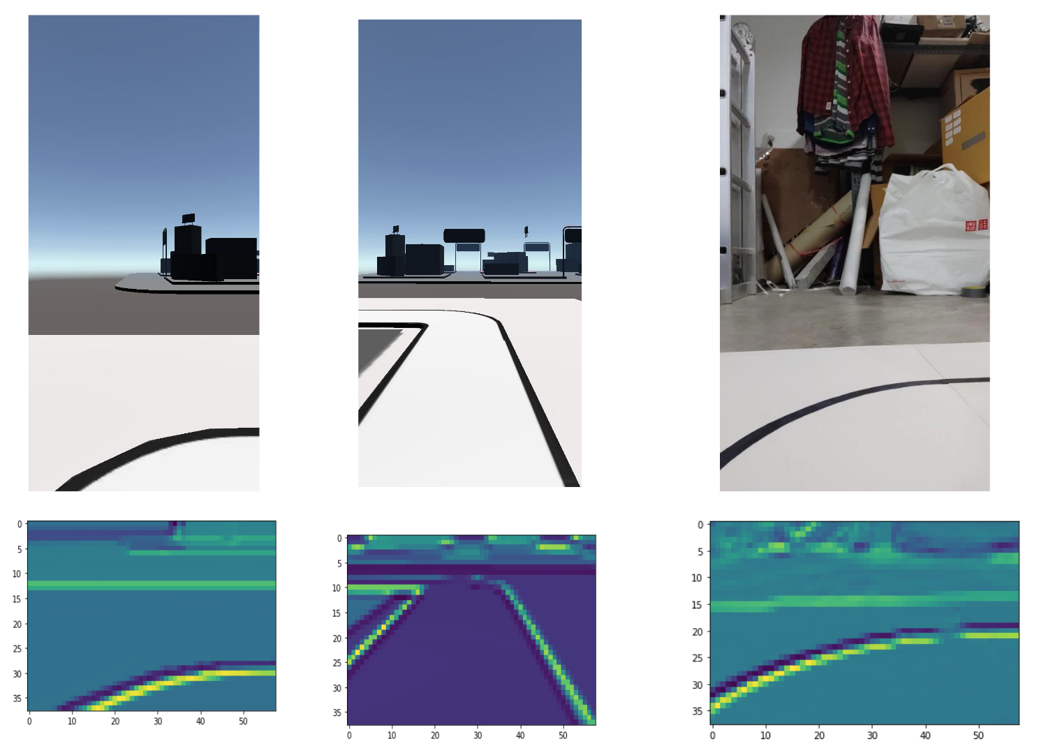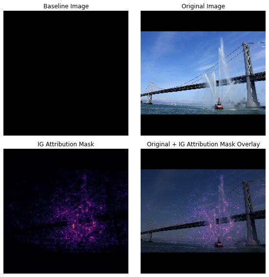
Output from the first Neural Network layer

Training the ML model using only the simulator doesn’t mean it will actually work in the real-world situation, at least not the first try. The car ran on the tracks for a few seconds and then just went off the track for various reasons.

Early versions of the toy car running off the track/td>

Later, we found out that we only trained the model using mostly straight tracks. To fix this imbalance data issue, we added various shapes of curves.

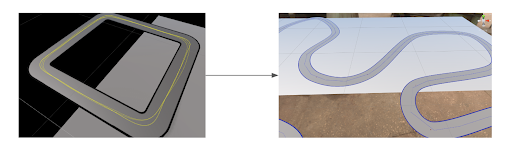(Left) square shape track, (Right) Curvy track

After fixing the imbalanced dataset, the car began to correctly navigate corners.

Car successfully turn at the corners

Training with the final track design

Final track design

We started creating more complex situations for the car, such as adding multiple intersections to the tracks. We also added more routing paths to make the car handle these new conditions. However, we ran into new problems right away which is the car turned and hit the side track when it tried to turn at the intersection because it saw some random objects outside the track.

Training the model with additional routing

We tested out many solutions and went with the one that was most simple and effective. We cropped only the bottom ¼ of the image and fed it to the lane keeping model, then adjusted the model input size to 120×40 and it works like a charm.

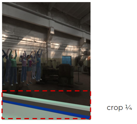Cropping bottom part of the image for lane-keeping

Object Detection

We use object detection for two purposes. One is for localization. Each car needs to know where it is in the city by detecting objects in its environment (in this case, we detect the traffic signs in the city). The other purpose is to detect other cars, so they won’t bump into each other.

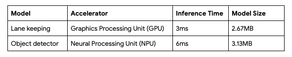
For choosing the object detector model there are many models already available in TensorFlow object detection model zoo. But, for the Pixel 4 edge TPU, we use the ssd_mobilenet_edgetpu model.

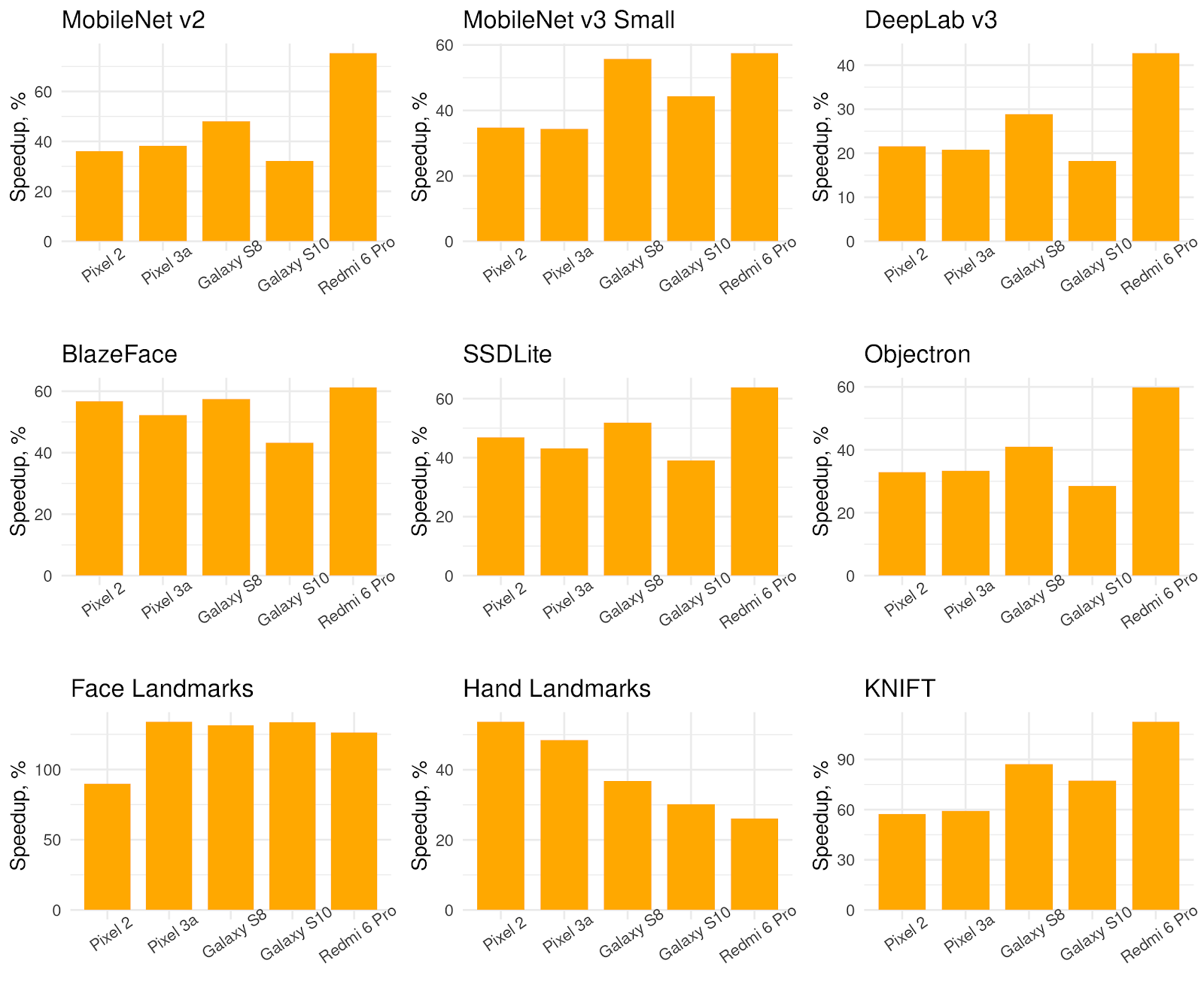
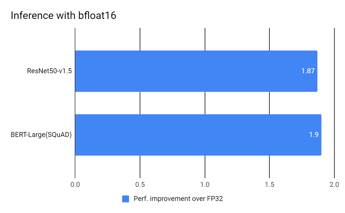
ssd_mobilenet_edgetpu model on Pixel 4’s “Neural Core” Edge TPU is currently the fastest mobilenet object detection. It takes only 6.6 ms per frame, which is more than enough for using with real-time applications.

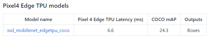Pixel 4 Edge TPU model performance

Data labelling and Simulation

We use image data from both simulation and real scenes to train the model. Next, we developed our own simulator for this using Unreal Engine 4. The simulator generates random objects with random background and also an annotation file in a Pascal VOC format that is used in TensorFlow object detection API.

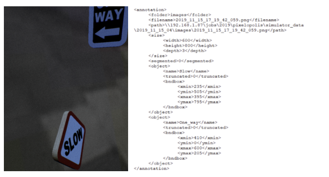Object detection simulator using UE4

For images that were taken from the real scene We have to do manual labeling using the labelImg tool.

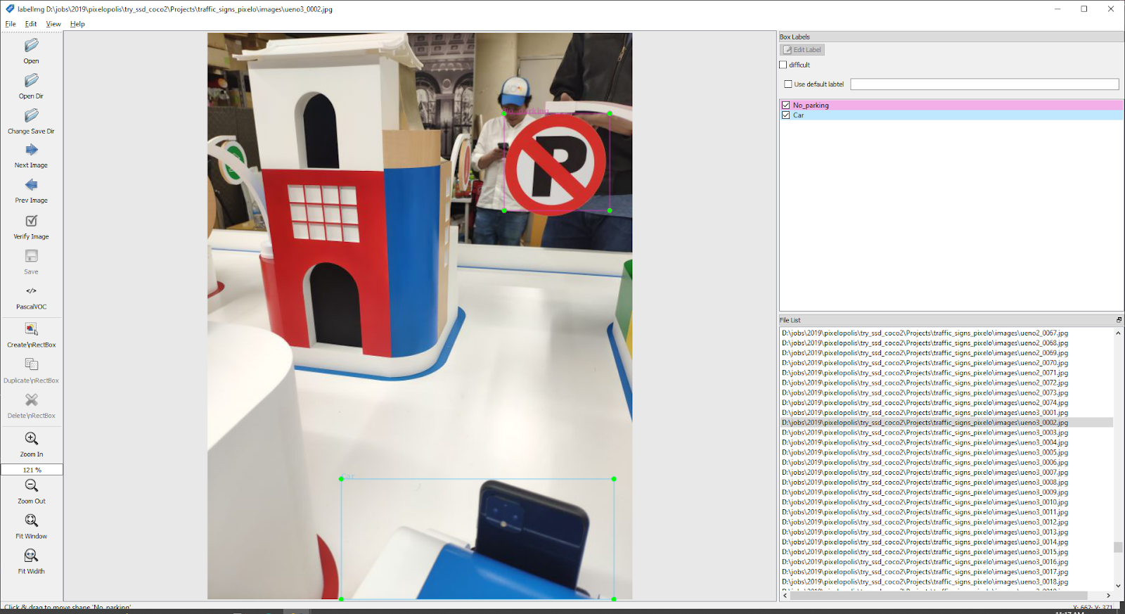Data labeling with labelImg

Training

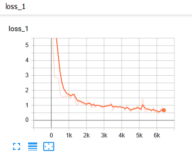Loss report

We used TensorBoard to monitor training progress. We use it to evaluate mAP (mean Average Precision), which normally you have to do it manually.

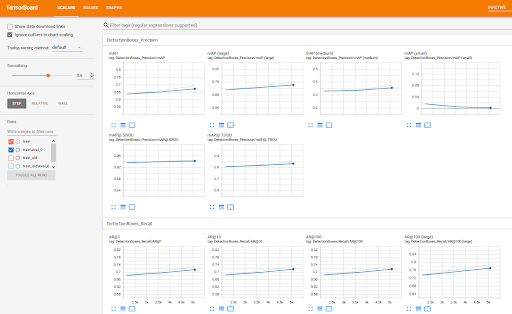TensorBoard

Detection result and the groundtruth

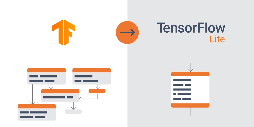
TensorFlow Lite

Since we want to run our ML model on the Pixel 4, which is running Android, we need to convert all the models to .tflite. Of course, you can use TensorFlow lite to target iOS and other devices as well (including microcontrollers). Here are the steps we did:

Lane keeping

First, we convert the lane keeping model from .h5 to .tflite by using

import tensorflow as tf
converter = tf.lite.TFLiteConverter.from_keras_model_file("lane_keeping.h5")
model = converter.convert()
file = open("lane_keeping.tflite",'wb') 
file.write( model )
file.close()

Now, we have the model ready for the Android project. Next, we build a lane keeping class in our app. We began with an example android project from here.

Object detection

We have to convert the model checkpoint (.ckpt) to tensorflow lite format (.tflite)

1. Using export_tflite_ssd_graph.py script to convert .ckpt to .pb file (the script already provided in Tensorflow object detector API)
2. Using toco: TensorFlow Lite Converter to convert .pb to .tflite format

Using Neural Core

We use an Android sample project from here. Then we modified the delegate to use Pixel 4 Edge TPU with the following code.

Interpreter.Options tfliteOptions = new Interpreter.Options();
nnApiDelegate = new NnApiDelegate();
tfliteOptions.addDelegate(nnApiDelegate);
tfLite = new Interpreter(loadModelFile(assetManager, modelFilename),tfliteOptions);

Real-time Video Streaming

After a user selects a destination, the car will start driving itself. While it’s driving, the car will stream what it sees to the station phone as a video feed. When we started implementing this part, we knew right away that streaming a raw video feed wouldn’t be possible due to the amount of data that we need to transfer between several car phones and station phones. The solution that we use is, first, compress a raw image frame to a JPEG format to reduce the amount of that data, then stream the JPEG buffer via http protocol using multipart/x-mixed-replace as an HTTP Content-type. This way we can achieve several video streams at the same time with unnoticeable lag between the devices.

Server App

Server Stack

We use NodeJS for the server app and MongoDB for the database.

Hail a Car

Since we have multiple stations and cars, we need to find a way to connect these two together. We built a booking system similar to popular car apps. Our booking system has 3 steps. First, the car connects to the server and tells the server that it’s ready to be booked. Second, the station connects to the server and asks the server for a car. Third, the server looks for the car that’s ready and connects these two together and also stores the device_id from both station and car apps.

Navigation

Node/Edge

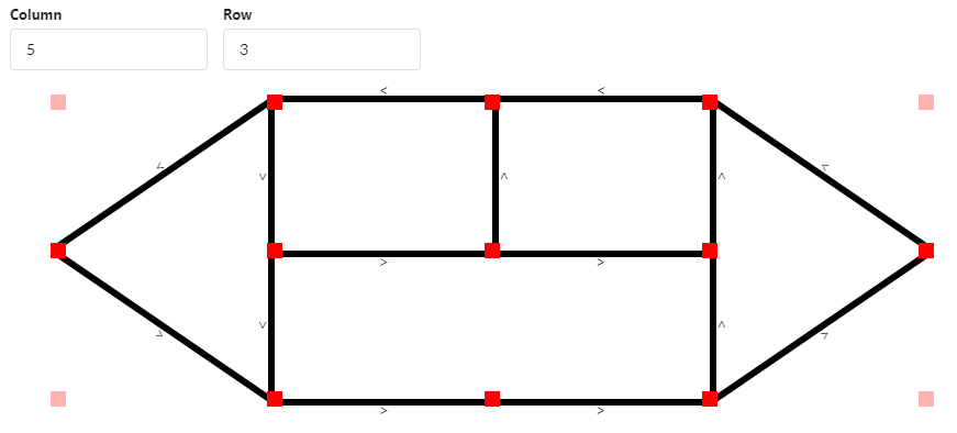
Since we will have a fleet of cars running around in the city, we need to find a way to navigate them. We use the Node/Edge concept. Node is a place on the map and Edge is the path between two Nodes. We then map each node to the actual signs in the city.

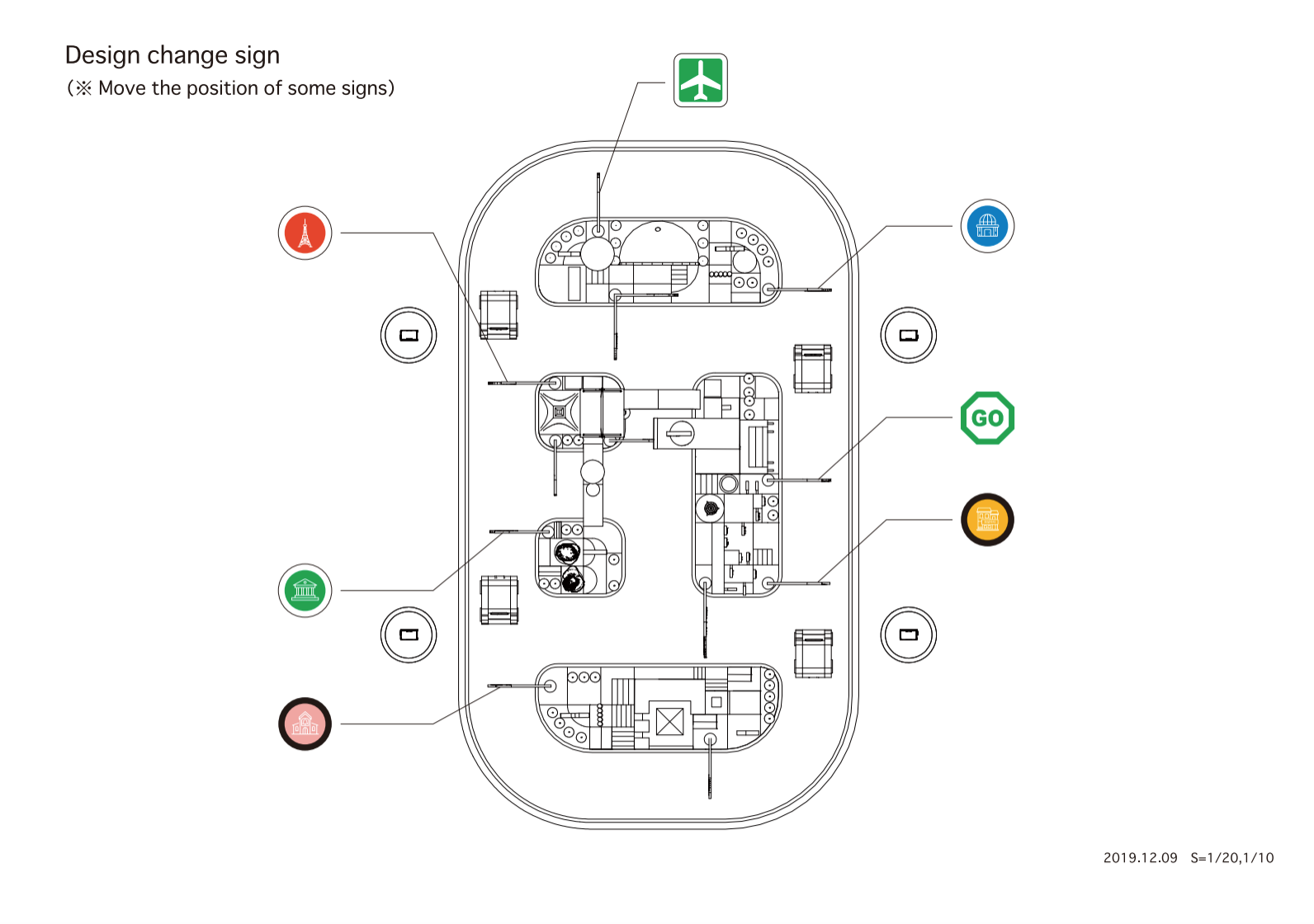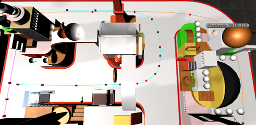
Top view of the tracks and sign locations

When the destination is selected on the station app, the station will send node_id to the server and the server will return an object which indicates a list of nodes and their properties so the car knows where to drive to and the expected sign it will see.

Electronics

Parts

We started off with NUCLEO-F411RE as our development board. We chose Dynamixel for the motors.

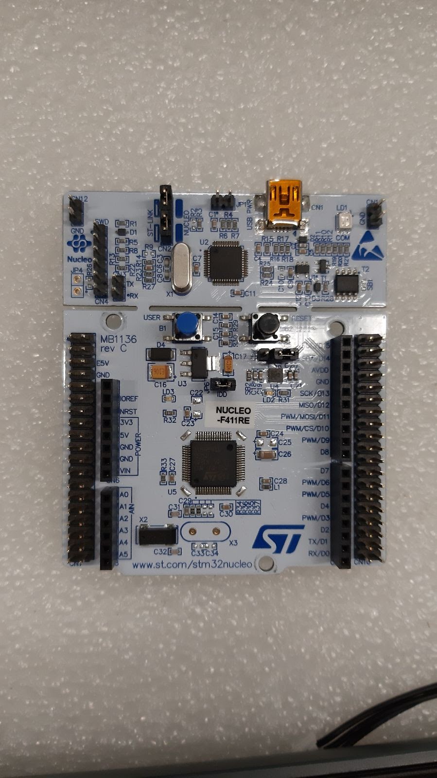NUCLEO-F411RE

We designed and developed a shield for additional components such as motors to reduce the number of wires inside the car chassis.There are three parts in the shield: 1) Battery measurement in voltage, 2) On/off switch with MOSFET, 3) Buttons.

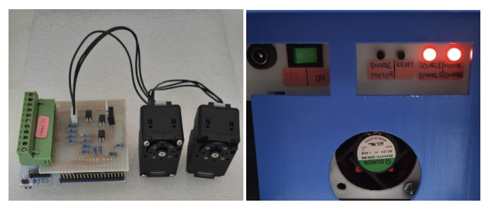(Left) Shield and Motors, (Right) Power socket, power switch, Enable motor button, Reset Motor button, Board status LED, Motor status LED

In the later phase, we would like to make the car a lot smaller, so we moved from NUCLEO-F411RE to NUCLEO-L432KC because it has a lot smaller footprint.

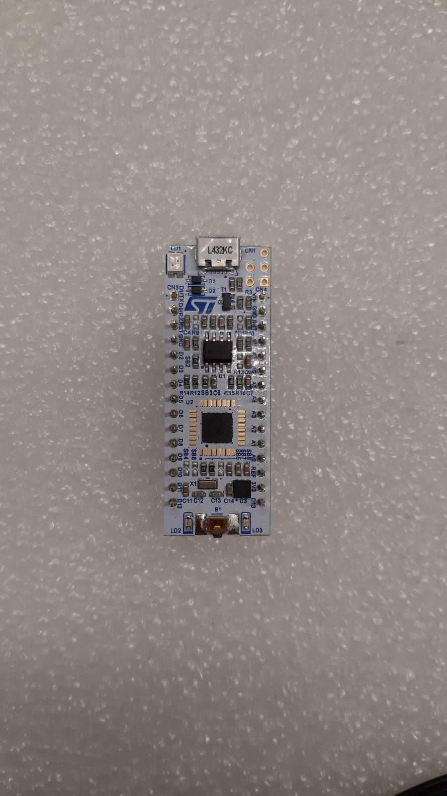NUCLEO-L432KC

Car Chassis & Exterior

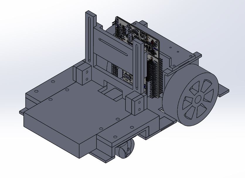
Mark I

Mark I Design

We designed and 3D printed the car chassis with PLA material. The front wheels are castor wheels.

Mark II

Mark II Design

We added a battery measurement circuit to the board and cut off the power when the phone detached from the board.

Mark III

Mark III Design

We added status LEDs so we can easily debug the state of the board. From the previous version, we encountered a motor overheating issue, so in this version we improved the ventilation by adding a fan to the motor. We also added a USB Type-C power delivery to the board so the phone can use the car battery.

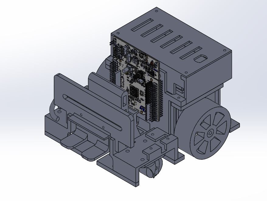
Mark IV

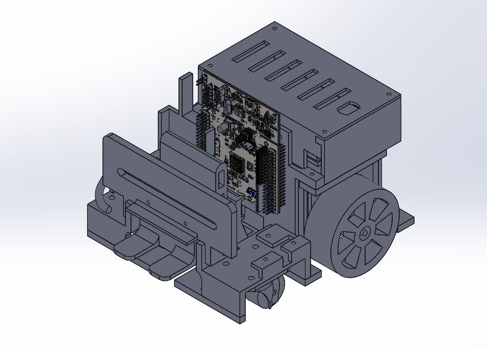Mark IV Design

We moved all the control buttons and status LEDs to the back of the car for an easy access.

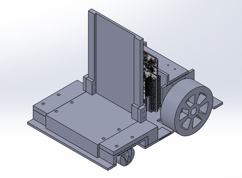
Mark V

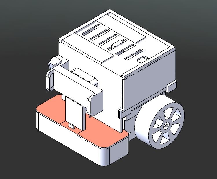Mark V Design

This is the final version and we need to reduce the car footprint as much as possible. First, we changed the board from NUCLEO-F411RE to NUCLEO-L432KC to achieve a smaller footprint. Second, the front wheel has been changed to ball caster wheels. Third, we rearranged the board location to the top of the car and stacked the battery underneath the board. Lastly, we removed the USB Type-C power delivery because we want to prolong the driving time by giving all battery power to the board and motors instead of the phone.

Performance metrics

Roadmap

There are many areas that we plan to improve this experience.

Battery

Currently, the motor and the controller board are powered by three packs of 3000mAh lithium-ion batteries and we have a charging circuit to handle the charging process. When we want to charge the battery, we would need to move the car to the charging station and plug the power adapter to the back of the car to charge. This has a lot of downsides because the car won’t be able to run on the track if it’s charging and the charging time is a few hours which is quite long.

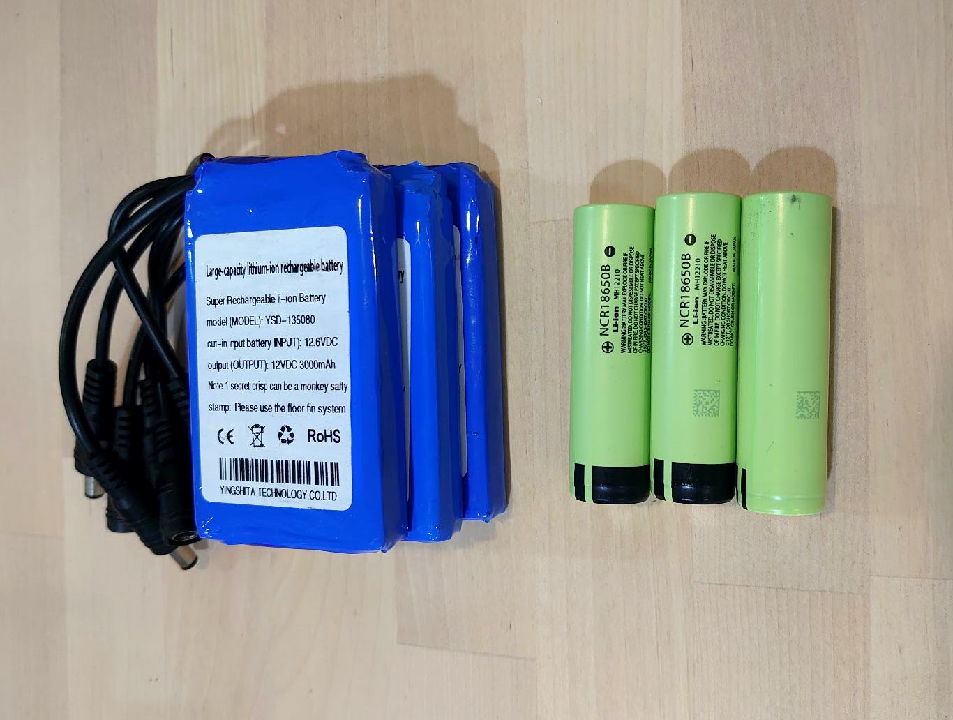3000mAh Li-ion Battery (left), 18650 Li-ion Battery (right)

We would like to reduce this process by changing the battery to an 18650 battery cell instead. This type of battery is used in electronics such as laptops, tools, and e-bikes, due to the high capacity in a small form factor. This way we can swap the battery easily by popping in the new ones and let the empty ones charge in the battery charger without leaving the car at the charging station.

Localization

Localization with SLAM

Localization is a very important process for this installation and we would like to make it more robust by adding SLAM to our app. We believe that this would improve the turning mechanism significantly.

Learning more

Thanks so much for reading! It’s incredible what you can do with a phone camera, TensorFlow and a bit of imagination. Hopefully, this post gave you ideas for your own projects – we learned a lot working on this one, and hope you will in yours as well. The article provides links to resources for you to delve deeper into all the different areas and you can find plenty of ML models and tutorials by the developer community to learn from on TensorFlow hub.
If you’re really passionate about building self-driving cars and want to learn more about how machine learning and deep learning are powering the autonomous vehicle industry check out Udemy’s Self Driving Cars Nanodegree Program. It’s perfect for engineers & students looking for complete training in all aspects of self-driving cars, including computer vision, sensor fusion & localization.

Acknowledgements

This project would not have been possible without the following awesome and talented group of people: Sina Hassani, Ashok Halambi, Pohung Chen, Eddie Azadi, Shigeki Hanawa, Clara Tan Su Yi, Daniel Bactol, Kiattiyot Panichprecha Praiya Chinagarn, Pittayathorn Nomrak, Nonthakorn Seelapun, Jirat Nakarit, Phatchara Pongsakorntorn, Tarit Nakavajara, Witsarut Buadit, Nithi Aiempongpaiboon, Witaya Junma, Taksapon Jaionnom and Watthanasuk Shuaytong.Read More

Posted by Vivek Rathod and Jonathan Huang, Google Research

At the TF Dev Summit earlier this year, we mentioned that we are making more of the TF ecosystem compatible so your favorite libraries and models work with TF 2.x. Today we are happy to announce that the TF Object Detection API (OD API) officially supports TensorFlow 2!

Over the last year we’ve been migrating our TF Object Detection API models to be TensorFlow 2 compatible. If you are a frequent visitor to the Object Detection API GitHub repository, you may have already seen bits and pieces of these new models. Our codebase offers tight Keras integration, access to distribution strategies, easy debugging with eager execution; all the goodies that one might expect from a TensorFlow 2 codebase. Specifically, this release includes:

• New binaries for train/eval/export that are eager mode compatible.
• A suite of TF2 compatible (Keras-based) models; this includes migrations of our most popular TF1 models (e.g., SSD with MobileNet, RetinaNet, Faster R-CNN, Mask R-CNN), as well as a few new architectures for which we will only maintain TF2 implementations: (1) CenterNet – a simple and effective anchor-free architecture based on the recent Objects as Points paper by Zhou et al, and (2) EfficientDet — a recent family of SOTA models discovered with the help of Neural Architecture Search.
• COCO pre-trained weights for all of the models provided as TF2 style object-based checkpoints
• Access to DistributionStrategies for distributed training: traditionally, we have mainly relied on asynchronous training for our TF1 models. We now support synchronous training as the primary strategy; Our TF2 models are designed to be trainable using sync multi-GPU and TPU platforms
• Colab demonstrations of eager mode compatible few-shot training and inference
• First-class support for keypoint estimation, including multi-class estimation, more data augmentation support, better visualizations, and COCO evaluation.

If you’d like to get your feet wet immediately, we recommend checking out our shiny new Colab demos (for inference and few-shot training). As a fun example, we’ve included a tutorial demonstrating how to train a rubber ducky detector using fine-tuning based few-shot training (with just five example images!).
Our philosophy for this migration was to expose all the benefits of TF2 and Keras, while continuing to support our wide user base still using TF1. We believe that there might be many teams out there grappling with similar migration projects, so we thought that a few words about our thought process and approach here might be useful even for non object-detection TensorFlow users.
Users to our codebase now belong to three categories: (1) New users who want to leverage new features (eager mode training, Distribution Strategies) and new models, (2) Existing TF1 users who want to migrate to TF2, and (3) Existing TF1 users who prefer not to migrate just yet. To support all three categories of users, we have followed a number of strategies detailed below:

• Refactor low-level core and meta-architecture to work in both TF1 and TF2. We realized most of our codebase could be shared across TF1 and TF2 (e.g., bounding box arithmetic, loss functions, input pipelines, visualization code, etc); where possible, we’ve tried to ensure that our code is agnostic about whether it is run under TF1 or TF2.
• Treat feature extractors/backbones as being specific to either TF1 or TF2. We continue to maintain our TF1 backbones which are implemented in tf-slim, and introduce TF2 backbones implemented in Keras. Then depending on the version of TensorFlow that a user is running, these models will be either enabled or disabled.
• Leverage community-maintained existing backbone implementations. Instead of re-implementing backbone architectures (e.g. MobileNet or ResNet) in Keras, our models depend on implementations in the Keras applications collection – a set of community-maintained canned architectures. We have also verified that our new Keras backbones maintain or surpass the accuracy of comparable tf-slim backbones (at least for the models that were already in the OD API).
• Increase unit test coverage to cover GPU/TPU, TF1 and TF2. Given that we now need to ensure functionality on multiple platforms (GPU and TPU) as well as across TF versions, we’ve designed a new and flexible unit testing framework that tests OD API functions under all four settings ({GPU, TPU}x{TF1, TF2}), while allowing for certain tests to be disabled (e.g. input pipelines are not tested on TPU)
• Separate front-end binaries (training loops, exporters) for TF1 and TF2. We have added a separate entry point for TF2 models (in the form of new TF2 training and export binaries) which can be run in eager mode, leveraging various DistributionStrategies.
• No changes to the frontend config language. In order to make migration from TF1 to TF2 as easy as possible for our users, we’ve worked hard to ensure that model specifications using OD API’s config language produce equivalent model architectures in both TF1 and TF2 and that models can be trained to the same level of numerical performance under both TF versions. As an example, if you have an existing ResNet-50 based RetinaNet model config that is trainable using TF1 binaries, then to train the same model with TF2 binaries, you would simply change the name of the feature extractor in the config (in this case from ssd_resnet50_v1_fpn to ssd_resnet50_v1_fpn_keras); all other hyperparameter specifications would remain unchanged.

This release is just one example of making the TF ecosystem TF2 compatible and easier to use. Over the next few months, we will continue to migrate large-scale codebases from TF1 to TF2. In addition, we are working to provide a more integrated, end-to-end experience in the TF ecosystem for researchers looking for easy-to-use modeling, starting with a unified computer vision library coming soon.
As always, please feel free to reach out with questions and feedback via GitHub. We appreciate help from the open source community. In particular, if you are a prior TF1.x user of the TensorFlow Object Detection API and there is a feature that you really like that you don’t see supported in the TF2 pipelines, we encourage you to let us know as this may help us to prioritize as we continue to release features/models.

Acknowledgements

This release is the result of a close collaboration among a number of teams within Google Research. In particular we want to highlight the contributions of the following individuals: first, a special thanks to Tomer Kaftan and Yanhui Liang for initiating this entire effort and doing most of the early heavy lifting. We also thank our main OD API contributors: Vighnesh Birodkar, Ronny Votel, Zhichao Lu, Yu-hui Chen, Sergi Caelles Prat, Jordi Pont-Tuset, Austin Myers. We are also grateful to many other contributors including: Sudheendra Vijayanarasimhan, Sara Beery, Shan Yang, Anjali Sridhar, Kathy Ruan, Karmel Allison, Allen Lavoie, Lu He, Yixin Shi, Derek Chow, David Ross, Pengchong Jin, Jaeyoun Kim, Jing Li, Mingxing Tan, Dan Kondratyuk, Kaushik Shivakumar, Yiming Shi and Tina Tian. Finally we also thank our interns and summer of code students for their contributions: Kathy Ruan, Kaushik Shivakumar, Yiming Shi, Vishnu Banna, Akhil Chinnakotla, and Anirudh Vegesana.Read More

Posted by Ashwin Murthy, Software Engineer, TensorFlow team @ Google

Overview

Efficiency and performance are critical for edge deployments. TensorFlow Lite achieves this by means of fusing and optimizing a series of more granular TensorFlow operations (which themselves are composed of composite operations, like LSTM) into a single executable TensorFlow Lite unit.

Many users have asked us for more granular control of the way operations can be fused to achieve greater performance improvements. Today, we are delivering just that by providing users with the ability to specify how operations can be fused.

Furthermore, this new capability allows for seamless conversion of TensorFlow Keras LSTM operations—one of our most requested features. And to top it off, you can now plug in a user-defined RNN conversion to TensorFlow Lite!

Fused operations are more efficient

As mentioned earlier, TensorFlow operations are typically composed of a number of primitive, more granular operations, such as tf.add. This is important in order to have a level of reusability, enabling users to create operations that are a composition of existing units. An example of a composite operation is tf.einsum. Executing a composite operation is equivalent to executing each of its constituent operations.

However, with efficiency in mind, it is common to “fuse” the computation of a set of more granular operations into a single operation.

Another use for fused operations is providing a higher level interface to define complex transformations like quantization, which would otherwise be infeasible or very hard to do at a more granular level.

Concrete examples of fused operations in TensorFlow Lite include various RNN operations like Unidirectional and Bidirectional sequence LSTM, convolution (conv2d, bias add, relu), fully connected (matmul, bias add, relu) and more.

Fusing TensorFlow operations into TensorFlow Lite operations has historically been challenging until now!

Out-of-the-box RNN conversion and other composite operation support

Out-of-the-box RNN conversion

We now support conversion of Keras LSTM and Keras Bidirectional LSTM, both of which are composite TensorFlow operations. This is the simplest way to get RNN-based models to take advantage of the efficient LSTM fused operations in TensorFlow Lite. See this notebook for end-to-end keras LSTM to TensorFlow Lite conversion and execution via the TensorFlow Lite interpreter.

Furthermore, we enabled conversion to any other TensorFlow RNN implementation by providing a convenient interface to the conversion infrastructure. You can see a couple of examples of this capability using lingvo’s LSTMCellSimple and LayerNormalizedLSTMCellSimple RNN implementations.

For more information, please look at our RNN conversion documentation.

Note: We are working on adding quantization support for TensorFlow Lite’s LSTM operations. This will be announced in the future.

Extending conversion to other composite operations

We extended the TensorFlow Lite converter to enable conversion of other composite TensorFlow operations into existing or custom TensorFlow Lite operations.

The following steps are needed to implement a TensorFlow operation fusion to TensorFlow Lite:

1. Wrap the composite operation in a tf.function. In the TensorFlow model source code, identify and abstract out the composite operation into a tf.function with the experimental_implements function annotation.
2. Write conversion code. Conceptually, the conversion code replaces the composite implementation of this interface with the fused one. In the prepare-composite-functions pass, plug in your conversion code.
3. Invoke the TensorFlow Lite converter. Use the TFLiteConverter.from_saved_model API to convert to TensorFlow Lite.

For the overall architecture of this infrastructure, see here. For detailed steps with code examples, see here. To learn how operation fusion works under the hood, see the detailed documentation.

Feedback

Please email tflite@tensorflow.org or create a GitHub issue with the component label “TFLiteConverter”.

Acknowledgements

This work would not have been possible without the efforts of Renjie Liu, a key collaborator on this project since its inception. We would like to thank Raziel Alvarez for his leadership and guidance. We would like to thank Jaesung Chung, Scott Zhu, Sean Silva, Mark Sandler, Andrew Selle, Qiao Liang and River Riddle for important contributions. We would like to acknowledge Sarah Sirajuddin, Jared Duke, Lawrence Chan, Tim Davis and the TensorFlow Lite team as well as Tatiana Shpeisman, Jacques Pienaar and the Google MLIR team for their active support of this work.Read More

Posted by Tulsee Doshi, Andrew Zaldivar

As billions of people around the world continue to use products or services with AI at their core, it becomes more important than ever that AI is deployed responsibly: preserving trust and putting each individual user’s well-being first. It has always been our highest priority to build products that are inclusive, ethical, and accountable to our communities, and in the last month, especially as the US has grappled with its history of systemic racism, that approach has been, and continues to be, as important as ever.

Two years ago, Google introduced its AI Principles, which guide the ethical development and use of AI in our research and products. The AI principles articulate our Responsible AI goals around privacy, accountability, security, fairness and interpretability. Each of these is a critical tenant in ensuring that AI-based products work well for every user.

As a Product Lead and Developer Advocate for Responsible AI at Google, we have seen first-hand how developers play an important role in building for Responsible AI goals using platforms like TensorFlow. As one of the most popular ML frameworks in the world, with millions of downloads and a global developer community, TensorFlow is not only used across Google, but around the globe to solve challenging real-world problems. This is why we’re continuing to expand the Responsible AI toolkit in the TensorFlow ecosystem, so that developers everywhere can better integrate these principles in their ML development workflows.

In this blog post, we will outline ways to use TensorFlow to build AI applications with Responsible AI in mind. The collection of tools here are just the beginning of what we hope will be a growing toolkit and library of lessons learned and resources to apply them.

You can find all the tools discussed below at TensorFlow’s collection of Responsible AI Tools.

Building Responsible AI with TensorFlow: A Guide

Building into the workflow

While every TensorFlow pipeline likely faces different challenges and development needs, there is a consistent workflow that we see developers follow as they build their own products. And, at each stage in this flow, developers face different Responsible AI questions and considerations. With this workflow in mind, we are designing our Responsible AI Toolkit to complement existing developer processes, so that Responsible AI efforts are directly embedded into a structure that is already familiar.

You can see a full summary of the workflow and tools at: tensorflow.org/resources/responsible-ai

To simplify our discussion, we’ll break the workflow into 5 key steps:

• Step 1: Define the problem
• Step 2: Collect and prepare the data
• Step 3: Build and train the model
• Step 4: Evaluate performance
• Step 5: Deploy and monitor

In practice, we expect that developers will move between these steps frequently. For example, a developer may train the model, identify poor performance, and return to collect and prepare additional data to account for these concerns. Likely, a model will be iterated and improved numerous times once it has been deployed and these steps will be repeated.
Regardless of when and the order in which you reach these steps, there are critical Responsible AI questions to ask at each phase—as well as related tools available to help developers debug and identify critical insights. As we go through each step in more detail, you will see several questions listed along with a set of tools and resources we recommend looking into in order to answer the questions raised. These questions, of course, are not meant to be comprehensive; rather, they serve as examples to stimulate thinking along the way.
Keep in mind that many of these tools and resources can be used throughout the workflow—not just exclusive for the step in which it is being featured. Fairness Indicators and ML Metadata, for example, can be used as standalone tools to respectively evaluate and monitor your model for unintended biases. These tools are also integrated in TensorFlow Extended, which provides a pathway for developers to not only put their model into production, but also equipping them with a unified platform to iterate through the workflow in a more seamless way.

Step 1: Define the Problem

What am I building? What is the goal?
Who am I building this for?
How are they going to use it? What are the consequences for the user when it fails?
The first step in any development process is the definition of the problem itself. When is AI actually a valuable solution, and what problem is it addressing? As you define your AI needs, make sure to keep in mind the different users you might be building for, and the different experiences they may have with the product.
For example, if you are building a medical model to screen individuals for a disease, as is done in this Explorable, the model may learn and work differently for adults versus children. When the model fails, it may have critical repercussions that both doctors and users need to know about.
How do you identify the important questions, potential harms, and opportunities for all users? The Responsible AI Toolkit in TensorFlow has a couple tools to help you:
PAIR Guidebook
The People + AI Research (PAIR) Guidebook, which focuses on designing human-centered AI, is a companion as you build, outlining the key questions to ask as you develop your product. It’s based on insights from Googlers across 40 product teams. We recommend reading through the key questions—and use the helpful worksheets!—as you define the problem, but referring back to these questions as development proceeds.
AI Explorables
A set of lightweight interactive tools, the Explorables provide an introduction to some of the key Responsible AI concepts.

Step 2: Collect & Prepare Data

Who does my dataset represent? Does it represent all my potential users?
How is my dataset being sampled, collected, and labeled?
How do I preserve the privacy of my users?
What underlying biases might my dataset encode?
Once you have defined the problem you seek to use AI to solve, a critical part of the process is collecting the data that best takes into account the societal and cultural factors necessary to solve the problem in question. Developers wanting to train, say, a speech detection model based on a very specific dialect might want to consider obtaining their data from sources that have gone through efforts in accommodating languages lacking linguistic resources.
As the heart and soul of an ML model, a dataset should be considered a product in its own right, and our goal is to equip you with the tools to understand who the dataset represents and what gaps may have existed in the collection process.
TensorFlow Data Validation
You can utilize TensorFlow Data Validation (TFDV) to analyze your dataset and slice across different features to understand how your data is distributed, and where there may be gaps or defects. TFDV combines tools such as TFX and Facets Overview to help you quickly understand the distribution of values across the features in your dataset. That way, you don’t have to create a separate codebase to monitor your training and production pipelines for skewness.

Example of a Data Card for the Colombian Spanish speaker dataset.

Analysis generated by TFDV can be used to create Data Cards for your datasets when appropriate. You can think about a Data Card as a transparency report for your dataset—providing insight into your collection, processing, and usage practices. As an example, one of our research-driven engineering initiatives focused on creating datasets for regions with both low resources for building natural language processing applications and rapidly growing Internet penetration. To help other researchers that desire to explore speech technology for these regions, the team behind this initiative created Data Cards for different Spanish speaking countries to start with, including the Colombian Spanish speaker dataset shown above, providing a template for what to expect when using their dataset.
Details on Data Cards, a framework on how to create them, and guidance on how to integrate aspects of Data Cards into processes or tools you use will be published soon.

Step 3: Build and Train the Model

How do I preserve privacy or think about fairness while training my model?
What techniques should I use?
Training your TensorFlow model can be one of the most complex pieces of the development process. How do you train it in such a way that it performs optimally for everyone while still preserving user privacy? We’ve developed a set of tools to simplify aspects of this workflow, and enable integration of best practices while you are setting up your TensorFlow pipeline:
TensorFlow Federated
Federated learning is a new approach to machine learning that enables many devices or clients to jointly train machine learning models while keeping their data local. Keeping the data local provides benefits around privacy, and helps protect against risks of centralized data collection, like theft or large-scale misuse. Developers can experiment with applying federated learning to their own models by using the TensorFlow Federated library.
[New] We recently released a tutorial for running high-performance simulations with TensorFlow Federated using Kubernetes clusters.
TensorFlow Privacy
You can also support privacy in training with differential privacy, which adds noise in your training to hide individual examples in the datasets. TensorFlow Privacy provides a set of optimizers that enable you to train with differential privacy, from the start.
TensorFlow Constrained Optimization and TensorFlow Lattice
In addition to building in privacy considerations when training your model, there may be a set of metrics that you want to configure and use in training machine learning problems to achieve desirable outcomes. Creating more equitable experiences across different groups, for example, is an outcome that may be difficult to achieve unless you consider taking into account a combination of metrics that satisfy this real-world requirement. The TFCO and TensorFlow
Lattice are libraries that provide a number of different research-based methods, enabling constraint-based approaches that could help you address broader societal issues such as fairness. In the next quarter, we hope to develop and offer more Responsible AI training methods, releasing infrastructure that we have used in our own products to work towards remediating fairness concerns. We’re excited to continue to build a suite of tools and case studies that show how different methods may be more or less suited to different use cases, and to provide opportunities for each case.

Step 4: Evaluate the Model

Is my model privacy preserving?
How is my model performing across my diverse user base?
What are examples of failures, and why are these occurring?
Once a model has been initially trained, the iteration process begins. Often, the first version of a model does not perform the way a developer hopes it would, and it is important to have easy to use tools to identify where it fails. It can be particularly challenging to identify what the right metrics and approaches are for understanding privacy and fairness concerns. Our goal is to support these efforts with tools that enable developers to evaluate privacy and fairness, in partnership with traditional evaluations and iteration steps.
[New] Privacy Tests
Last week, we announced a privacy testing library as part of TensorFlow Privacy. This library is the first of many tests we hope to release to enable developers to interrogate their models and identify instances where a single datapoint’s information has been memorized and might warrant further analysis on the part of the developer, including the consideration to train the model to be differentially private.
Evaluation Tool Suite: Fairness Indicators, TensorFlow Model Analysis, TensorBoard, and What-If Tool
You can also explore TensorFlow’s suite of evaluation tools to understand fairness concerns in your model and debug specific examples.
Fairness Indicators enables evaluation of common fairness metrics for classification and regression models on extremely large datasets. The tool is accompanied by a series of case studies to help developers easily identify appropriate metrics for their needs and set up Fairness Indicators with a TensorFlow model. Visualizations are available via the widely popular TensorBoard platform that modelers already use to track their training metrics. Most recently, we launched a case study highlighting how Fairness Indicators can be used with pandas, to enable evaluations over more datasets and data types.
Fairness Indicators is built on top of TensorFlow Model Analysis (TFMA), which contains a broader set of metrics for evaluating common metrics across concerns.

The What-If Tool lets you test hypothetical situtations on datapoints.

Once you’ve identified a slice that isn’t performing well or want to understand and explain errors more carefully, you can further evaluate your model with the What-If Tool (WIT), which can be used directly from Fairness Indicators and TFMA. With the What-if Tool, you can deepen your analysis on your specific slice of data by inspecting the model predictions at the datapoint level. The tool offers a large range of features, from testing hypothetical situations on datapoint, such as “what if this datapoint was from a different category?”, to visualizing the importance of different data features to your model’s prediction.
Beyond the integration in Fairness Indicators, the What-If Tool can also be used in other user flows as a standalone tool and is accessible from TensorBoard or in Colaboratory, Jupyter and Cloud AI Platform notebooks.
[New] Today, to help WIT users get started faster, we’re releasing a series of new educational tutorials and demos to help our users better use the tool’s numerous capabilities, from making good use of counterfactuals to interpret your model behaviors, to exploring your features and identifying common biases.
Explainable AIGoogle Cloud users can take WIT’s capabilities a step further with Explainable AI, a toolkit that builds upon WIT to introduce additional interpretability features including Integrated Gradients, which identify the features that most significantly impacted model performance.
Tutorials on TensorFlow.orgYou may also be interested in these tutorials for handling imbalanced datasets, and for explaining an image classifier using Integrated Gradients, similar to that mentioned above.

Using the tutorial above to explain why this image was classified as a fireboat (it’s likely because of the water spray).

Step 5: Deploy and Monitor

How does my model perform overtime? How does it perform in different scenarios? How do I continue to track and improve its progress?
No model development process is static. As the world changes, users change, and so do their needs. The model discussed earlier to screen patients, for example, may no longer work effectively during a pandemic. It’s important that developers have tools that enable tracking of models, and clear channels and frameworks for communicating helpful details about their models, especially to developers who may inherit a model, or to users and policy makers who seek to understand how it will work for various people. The TensorFlow ecosystem has tools to help with this kind of lineage tracking and transparency:
ML Metadata
As you design and train your model, you can allow ML Metadata (MLMD) to generate trackable artifacts throughout your development process. From your training data ingestion and any metadata around the execution of the individual steps, to exporting your model with evaluation metrics and accompanying context such as changelists and owners, the MLMD API can create a trace of all the intermediate components of your ML workflow. This ongoing monitoring of progress that MLMD provides helps identify security risks or complications in training.
Model Cards
As you deploy your model, you could also accompany its deployment with a Model Card—a document structured in a format that serves as an opportunity for you to communicate the values and limitations of your model. Model Cards could enable developers, policy makers, and users to understand aspects about trained models, contributing to the larger developer ecosystem with added clarity and explainability so that ML is less likely to be used in contexts for which it is inappropriate. Based on a framework proposed in an academic paper by Google researchers published in early 2019, Model Cards have since been released with Google Cloud Vision API models, including their Object and Face Detection APIs, as well as a number of open source models.
Today, you can get inspiration from the paper and existing examples to develop your own Model Card. In the next two months, we plan to combine ML Metadata and the Model Card framework to provide developers with a more automated way of creating these important artifacts. Stay tuned for our Model Cards Toolkit, which we will add to the Responsible AI Toolkit collection.

Excited to try out these resources? You can find all of them at tensorflow.org/resources/responsible-ai

It’s important to note that while Responsible AI in the ML workflow is a critical factor, building products with AI ethics in mind is a combination of technical, product, policy, process, and cultural factors. These concerns are multifaceted and fundamentally sociotechnical. Issues of fairness, for example, can often be traced back to histories of bias in the world’s underlying systems. As such, proactive AI responsibility efforts not only require measurement and modelling adjustments, but also policy and design changes to provide transparency, rigorous review processes, and a diversity of decision makers who can bring in multiple perspectives.
This is why many of the tools and resources we covered in this post are founded in the sociotechnical research work we do at Google. Without such a robust foundation, these ML and AI models are bound to be ineffective in benefiting society as they could erroneously become integrated into the entanglements of decision-making systems. Adopting a cross-cultural perspective, grounding our work in human-centric design, extending transparency towards all regardless of expertise, and operationalizing our learnings into practices—these are some of the steps we take to responsibly build AI.
We understand Responsible AI is an evolving space that is critical, which is why we are hopeful when we see how the TensorFlow community is thinking about the issues we’ve discussed—and more importantly, when the community takes action. In our latest Dev Post Challenge, we asked the community to build something great with TensorFlow incorporating AI Principles. The winning submissions explored areas of fairness, privacy, and interpretability, and showed us that Responsible AI tools should be well integrated into TensorFlow ecosystem libraries. We will be focusing on this to ensure these tools are easily accessible.
As you begin your next TensorFlow project, we encourage you to use the tools above, and to provide us feedback at tf-responsible-ai@google.com. Share your learnings with us, and we’ll continue to do the same, so that we can together build products that truly work well for everyone.
Read More

Posted by Khanh LeViet, TensorFlow Developer Advocate

TensorFlow Lite is the official framework for running TensorFlow models on mobile and edge devices. It is used in many of Google’s major mobile apps, as well as applications by third-party developers. When deploying TensorFlow Lite models in production, you may come across situations where you need some support features that are not provided out-of-the-box by the framework, such as:

• over-the-air deployment of TensorFlow Lite models
• measure model inference speed in user devices
• A/B test multiple model versions in production

In these cases, instead of building your own solutions, you can leverage Firebase to quickly implement these features in just a few lines of code.
Firebase is the comprehensive app development platform by Google, which provides you infrastructure and libraries to make app development easier for both Android and iOS. Firebase Machine Learning offers multiple solutions for using machine learning in mobile applications.
In this blog post, we show you how to leverage Firebase to enhance your deployment of TensorFlow Lite models in production. We also have codelabs for both Android and iOS to show you step-by-step of how to integrate the Firebase features into your TensorFlow Lite app.

Deploy model over-the-air instantly

You may want to deploy your machine learning model over-the-air to your users instead of bundling it into your app binary. For example, the machine learning team who builds the model has a different release cycle with the mobile app team and they want to release new models independently with the mobile app release. In another example, you may want to lazy-load machine learning models, to save device storage for users who don’t need the ML-powered feature and reduce your app size for faster download from Play Store and App Store.
With Firebase Machine Learning, you can deploy models instantly. You can upload your TensorFlow Lite model to Firebase from the Firebase Console. You can also upload your model to Firebase using the Firebase ML Model Management API. This is especially useful when you have a machine learning pipeline that automatically retrains models with new data and uploads them directly to Firebase. Here is a code snippet in Python to upload a TensorFlow Lite model to Firebase ML.

# Load a tflite file and upload it to Cloud Storage.
source = ml.TFLiteGCSModelSource.from_tflite_model_file('example.tflite')

# Create the model object.
tflite_format = ml.TFLiteFormat(tflite_source=source)
model = ml.Model(display_name="example_model", model_format=tflite_format)

# Add the model to your Firebase project and publish it.
new_model = ml.create_model(model)
ml.publish_model(new_model.model_id)

Once your TensorFlow Lite model has been uploaded to Firebase, you can download it in your mobile app at any time and initialize a TensorFlow Lite interpreter with the downloaded model. Here is how you do it on Android.

val remoteModel = FirebaseCustomRemoteModel.Builder("example_model").build()

// Get the last/cached model file.
FirebaseModelManager.getInstance().getLatestModelFile(remoteModel)
  .addOnCompleteListener { task ->
    val modelFile = task.result
    if (modelFile != null) {
      // Initialize a TF Lite interpreter with the downloaded model.
      interpreter = Interpreter(modelFile)
    }
  }

Measure inference speed on user devices

There is a diverse range of mobile devices available in the market nowadays, from flagship devices with powerful chips optimized to run machine learning models to cheap devices with low-end CPUs. Therefore, your model inference speed on your users’ devices may vary largely across your user base, leaving you wondering if your model is too slow or even unusable for some of your users with low-end devices.
You can use Performance Monitoring to measure how long your model inference takes across all of your user devices. As it is impractical to have all devices available in the market for testing in advance, the best way to find out about your model performance in production is to directly measure it on user devices. Firebase Performance Monitoring is a general purpose tool for measuring performance of mobile apps, so you also can measure any arbitrary process in your app, such as pre-processing or post-processing code. Here is how you do it on Android.

// Initialize a Firebase Performance Monitoring trace
val modelInferenceTrace = firebasePerformance.newTrace("model_inference")

// Run inference with TensorFlow Lite
interpreter.run(...)

// End the Firebase Performance Monitoring trace
modelInferenceTrace.stop()

Performance data measured on each user device is uploaded to Firebase server and aggregated to provide a big picture of your model performance across your user base. From the Firebase console, you can easily identify devices that demonstrate slow inference, or see how inference speed differs between OS versions.

A/B test multiple model versions

When you iterate on your machine learning model and come up with an improved model, you may feel very eager to release it to a production right away. However, it is not rare that a model may perform well on test data but fail badly in production. Therefore, the best practice is to roll out your model to a smaller set of users, A/B test it with the original model and closely monitor how it affects your important business metrics before releasing it to all of your users.
Firebase A/B Testing enables you to run this kind of A/B testing with minimal effort. The steps required are:

1. Upload all TensorFlow Lite model versions that you want to test to Firebase, giving each one a different name.
2. Setup Firebase Remote Config in the Firebase console to manage the TensorFlow Lite model name used in the app.
   • Update the client app to fetch TensorFlow Lite model name from Remote Config and download the corresponding TensorFlow Lite model from Firebase.
3. Setup A/B testing in the Firebase console.
   • Decide the testing plan (e.g. how many percent of your user base to test each model version).
   • Decide the metric(s) that you want to optimize for (e.g. number of conversions, user retention etc.).

Here is an example of setting up an A/B test with TensorFlow Lite models. We deliver each of two versions of our model to 50% of our user base and with the goal of optimizing for multiple metrics. Then we change our app to fetch the model name from Firebase and use it to download the TensorFlow Lite model assigned to each device.

val remoteConfig = Firebase.remoteConfig
remoteConfig.fetchAndActivate()
  .addOnCompleteListener(this) { task ->
      // Get the model name from Firebase Remote Config
      val modelName = remoteConfig["model_name"].asString()
      
      // Download the model from Firebase ML
      val remoteModel = FirebaseCustomRemoteModel.Builder(modelName).build()
      val manager = FirebaseModelManager.getInstance()
      manager.download(remoteModel).addOnCompleteListener {
        // Initialize a TF Lite interpreter with the downloaded model
        interpreter = Interpreter(modelFile)
      }
  }

After you have started the A/B test, Firebase will automatically aggregate the metrics on how your users react to different versions of your model and show you which version performs better. Once you are confident with the A/B test result, you can roll out the better version to all of your users with just one click.

Next steps

Check out this codelab (Android version or iOS version) to learn step by step how to integrate these Firebase features into your app. It starts with an app that uses a TensorFlow Lite model to recognize handwritten digits and show you:

• How to upload a TensorFlow Lite model to Firebase via the Firebase Console and the Firebase Model Management API.
• How to dynamically download a TensorFlow Lite model from Firebase and use it.
• How to measure pre-processing, post processing and inference time on user devices with Firebase Performance Monitoring.
• How to A/B test two versions of a handwritten digit classification model with Firebase A/B Testing.

Acknowledgements

Amy Jang, Ibrahim Ulukaya, Justin Hong, Morgan Chen, Sachin KotwaniRead More

Posted by Shuang Song and David Marn

Overview of a membership inference attack. An attacker tries to figure out whether certain examples were part of the training data.

Today, we’re excited to announce a new experimental module in TensorFlow Privacy (GitHub) that allows developers to assess the privacy properties of their classification models.

Privacy is an emerging topic in the Machine Learning community. There aren’t canonical guidelines to produce a private model. There is a growing body of research showing that a machine learning model can leak sensitive information of the training dataset, thus creating a privacy risk for users in the training set.

Last year, we launched TensorFlow Privacy, enabling developers to train their models with differential privacy. Differential privacy adds noise to hide individual examples in the training dataset. However, this noise is designed for academic worst-case scenarios and can significantly affect model accuracy.

These challenges led us to tackle privacy from a different perspective. A few years ago, research around the privacy properties of machine learning models started to emerge. Cost-efficient “membership inference attacks” predict whether a specific piece of data was used during training. If an attacker is able to make a prediction with high accuracy, they will likely succeed in figuring out if a data piece was used in the training set. The biggest advantage of a membership inference attack is that it is easy to perform, i.e., does not require any re-training.

A test produces a vulnerability score that determines whether the model leaks information from the training set. We found that this vulnerability score often decreases with heuristics, such as early stopping or using DP-SGD for training.

Membership inference attack on models for CIFAR10. The x-axis is the test accuracy of the model, and y-axis is vulnerability score (lower means more private). Vulnerability grows while test accuracy remains the same – better generalization could prevent privacy leakage.

Unsurprisingly, differential privacy helps in reducing these vulnerability scores. Even with very small amounts of noise, the vulnerability score decreased.

After using membership inference tests internally, we’re sharing them with developers to help them build more private models, explore better architecture choices, use regularization techniques such as early stopping, dropout, weight decay, and input augmentation, or collect more data. Ultimately, these tests can help the developer community identify more architectures that incorporate privacy design principles and data processing choices.

We hope this library will be the starting point of a robust privacy testing suite that can be used by any machine learning developer around the world. Moving forward, we’ll explore the feasibility of extending membership inference attacks beyond classifiers and develop new tests. We’ll also explore adding this test to the TensorFlow ecosystem by integrating with TFX.

Reach out to tf-privacy@google.com and let us know how you’re using this new module. We’re keen on hearing your stories, feedback, and suggestions!

Acknowledgments: Yurii Sushko, Andreas Terzis, Miguel Guevara, Niki Kilbertus, Vadym Doroshenko, Borja De Balle Pigem, Ananth Raghunathan. Read More

A guest post by Niranjan Hasabnis, Mohammad Ashraf Bhuiyan, Wei Wang, AG Ramesh at Intel
The recent growth of Deep Learning has driven the development of more complex models that require significantly more compute and memory capabilities. Several low precision numeric formats have been proposed to address the problem. Google’s bfloat16 and the FP16: IEEE half-precision format are two of the most widely used sixteen bit formats. Mixed precision training and inference using low precision formats have been developed to reduce compute and bandwidth requirements.

Bfloat16, originally developed by Google and used in TPUs, uses one bit for sign, eight for exponent, and seven for mantissa. Due to the greater dynamic range of bfloat16 compared to FP16, bfloat16 can be used to represent gradients directly without the need for loss scaling. In addition, it has been shown that mixed precision training using bfloat16 can achieve the same state-of-the-art (SOTA) results across several models using the same number of iterations as FP32 and with no changes to hyper-parameters.

The recently launched 3^rd Gen Intel^® Xeon^® Scalable processor (codenamed Cooper Lake), featuring Intel^® Deep Learning Boost, is the first general-purpose x86 CPU to support the bfloat16 format. Specifically, three new bfloat16 instructions are added as a part of the AVX512_BF16 extension within Intel Deep Learning Boost: VCVTNE2PS2BF16, VCVTNEPS2BF16, and VDPBF16PS. The first two instructions allow converting to and from bfloat16 data type, while the last one performs a dot product of bfloat16 pairs. Further details can be found in the hardware numerics document published by Intel.

Intel has worked with the TensorFlow development team to enhance TensorFlow to include bfloat16 data support for CPUs. We are happy to announce that these features are now available in the Intel-optimized buildof TensorFlow on github.com. Developers can use the latest Intel build of TensorFlow to execute their current FP32 models using bfloat16 on 3^rd Gen Intel Xeon Scalable processors with just a few code changes.

Using bfloat16 with Intel-optimized TensorFlow.

Existing TensorFlow 1 FP32 models (or TensorFlow 2 models using v1 compat mode) can be easily ported to use the bfloat16 data type to run on Intel-optimized TensorFlow. This can be done by enabling a graph rewrite pass (AutoMixedPrecisionMkl). The rewrite optimization pass will automatically convert certain operations to bfloat16 while keeping some in FP32 for numerical stability. In addition, models can also be manually converted by following instructions provided by Google for running on the TPU. However, such manual porting requires a good understanding of the model and can prove to be cumbersome and error prone.

TensorFlow 2 has a Keras mixed precision API that allows model developers to use mixed precision for training Keras models on GPUs and TPUs. We are currently working on supporting this API in Intel optimized TensorFlow for 3rd Gen Intel Xeon Scalable processors. This feature will be available in TensorFlow master branch later this year. Once available, we recommend users use the Keras API over the grappler pass, as the Keras API is more flexible and supports Eager mode.

Performance improvements.

We investigated the performance improvement of mixed precision training and inference with bfloat16 on 3 models – ResNet50v1.5, BERT-Large (SQuAD), and SSD-ResNet34. ResNet50v1.5 is a widely tested image classification model that has been included in MLPerf for benchmarking different hardware on vision workloads. BERT-Large (SQuAD) is a fine-tuning task that focuses on reading comprehension and aims to answer questions given a text/document. SSD-ResNet34 is an object detection model that uses ResNet34 as a backbone model.

The bfloat16 models were benchmarked on a 4 socket system with 3rd Gen Intel Xeon Scalable Processors with 28 cores* and compared with FP32 performance of a 4 socket system with 28 core 2nd Gen Intel Xeon Scalable Processors.


As shown in the charts above, training the models with mixed precision on a 3rd Gen Intel Xeon Scalable Processors with bfloat16 was 1.7x to 1.9x faster than FP32 precision on a 2nd Gen Intel Xeon Scalable Processors. Similarly, for inference, using bfloat16 precision resulted in a 1.87x to 1.9x performance increase.

Accuracy and time to train

In addition to performance measurements, we performed full convergence tests for the three deep learning models on two multi socket 3rd Gen Intel Xeon Scalable processor based systems*. For BERT-Large (SQuAD) and SSD-ResNet34, 4 socket 28 core systems were used. For ResNet50v1.5, we used an 8-socket 28 core system of 3rd Gen Intel Xeon Scalable processors. The models were first trained with FP32, and exactly the same hyper-parameters (learning rate etc.) and batch sizes were used to train the model with mixed precision.
The results above show that the models from three different use cases (image classification, language modeling, and object detection) are all able to reach SOTA accuracy using the same number of epochs. For ResNet50v1.5, the standard MLPerf threshold of 75.9% top-1 accuracy was used and both bfloat16 and FP32 reached the target accuracy in 84th epochs (evaluation every 4 epochs with eval offset of 0). For BERT-Large (SQuAD) fine-tuning task, both Bfloat16 and FP32 used two epochs. SSD-ResNet34, trained in 60 epochs. With the improved run time performance, the total time to train with bfloat16 was 1.7x to 1.9x better than the training time in FP32.

Intel-optimized Community build of TensorFlow

The Intel-optimized build of TensorFlow now supports Intel® Deep Learning Boost’s new bfloat16 capability for mixed precision training and low precision inference in the TensorFlow GitHub master branch. More information on the Intel build is available here. The models mentioned in this blog and scripts to run the models in bfloat16 and FP32 mode are available through the Model Zoo for Intel Architecture (v1.6.1 or later), which you can download and try from here. [Note: To run a bfloat16 model, you will need a Intel Xeon Scalable processor (Skylake) or later generation Intel Xeon Processor. However, to get the best performance of bfloat16 models, you will need a 3^rd Gen Intel Xeon Scalable processor.]

Conclusion

As deep learning models get larger and more complicated, the combination of the latest 3rd Gen Intel Xeon Scalable processors with Intel Deep Learning Boost’s new bfloat16 format can achieve a performance increase of up to 1.7x to 1.9x over FP32 performance on 2nd Gen Intel® Xeon® Scalable Processors, without any loss of accuracy. We have enhanced the Intel -optimized build of TensorFlow so developers can easily port their models to use mixed precision training and inference with bfloat16. In addition, we have shown that the automatically-converted bfloat16 model does not need any additional tuning of hyperparameters to converge; you canuse the same set of hyperparameters that you used to train the FP32 models.

Acknowledgements

The results presented in this blog is the work of many people including the Intel TensorFlow and oneDNN teams and our collaborators in Google’s TensorFlow team.

From Intel – Jojimon Varghese , Xiaoming Cui, Md Faijul Amin, Niroop Ammbashankar, Mahmoud Abuzaina, Sharada Shiddibhavi, Chuanqi Wang, Yiqiang Li, Yang Sheng, Guizi Li, Teng Lu, Roma Dubstov, Tatyana Primak, Evarist Fomenko, Igor Safonov, Abhiram Krishnan, Shamima Najnin, Rajesh Poornachandran, Rajendrakumar Chinnaiyan.

From Google – Reed Wanderman-Milne, Penporn Koanantakool, Rasmus Larsen, Thiru Palaniswamy, Pankaj Kanwar.

*For configuration details see www.intel.com/3rd-gen-xeon-configs.

Notices and Disclaimers

Intel’s compilers may or may not optimize to the same degree for non-Intel microprocessors for optimizations that are not unique to Intel microprocessors. These optimizations include SSE2, SSE3, and SSSE3 instruction sets and other optimizations. Intel does not guarantee the availability, functionality, or effectiveness of any optimization on microprocessors not manufactured by Intel. Microprocessor-dependent optimizations in this product are intended for use with Intel microprocessors. Certain optimizations not specific to Intel microarchitecture are reserved for Intel microprocessors. Please refer to the applicable product User and Reference Guides for more information regarding the specific instruction sets covered by this notice.
Read More

Posted by Luiz Gustavo Martins, Beat Gfeller and Christian Frank

Pitch is an attribute of musical tones (along with duration, intensity and timbre) that allows you to describe a note as “high” or “low”. Pitch is quantified by frequency, measured in Hertz (Hz), where one Hz corresponds to one cycle per second. The higher the frequency, the higher the note.

Pitch detection is an interesting challenge. Historically, for a machine to understand pitch, it would need to rely on complex hand-crafted signal-processing algorithms to measure the frequency of a note, in particular to separate the relevant frequency from background noise and backing instruments. Today, we can do that with machine learning, more specifically with the SPICE model (SPICE: Self-Supervised Pitch Estimation).

SPICE is a pretrained model that can recognize the fundamental pitch from mixed audio recordings (including noise and backing instruments). The model is also available to use on the web with TensorFlow.js and on mobile devices with TensorFlow Lite.

In this tutorial, we’ll walk you through using SPICE to extract the pitch from short musical clips. First we will load the audio file and process it. Then we will use machine learning to solve this problem (and you’ll notice how easy it is with TensorFlow Hub). Finally, we will do some post-processing and some cool visualization. You can follow along with this Colab notebook.

Loading the audio file

The model expects raw audio samples as input. To help you with this, we’ve shown four methods you can use to import your input wav file to the colab:

1. Record a short clip of yourself singing directly in Colab
2. Upload a recording from your computer
3. Download a file from your Google Drive
4. Download a file from a URL

You can choose any one of these methods. Recording yourself singing directly in Colab is the easiest one to try, and the most fun.
Audio can be recorded in many formats (for example, you might record using an Android app, or on a desktop computer, or on the browser), converting your audio into the exact format the model expects can be challenging. To help you with that, there’s a helper function convert_audio_for_model to convert your wav file to the correct format of one audio channel at 16khz sampling rate.
For the rest of this post, we will use this file:

Preparing the audio data

Now that we have loaded the audio, we can visualize it using a spectrogram, which shows frequencies over time. Here, we use a logarithmic frequency scale, to make the singing more clearly visible (note that this step is not required to run the model, it is just for visualization).

Note: this graph was created using Librosa lib. You can find more information here.

We need one last conversion. The input must be normalized to floats between -1 and 1. In a previous step we converted the audio to be in 16 bit format (using the helper function convert_audio_for_model). To normalize it, we just need to divide all the values by 2¹⁶ or in our code, MAX_ABS_INT16:

audio_samples = audio_samples / float(MAX_ABS_INT16)

Executing the model

Loading a model from TensorFlow Hub is simple. You just use the load method with the model’s URL.

model = hub.load("https://tfhub.dev/google/spice/2")

Note: An interesting detail here is that all the model urls from Hub can be used for download and also to read the documentation, so if you point your browser to that link, you can read documentation on how to use the model and learn more about how it was trained.
Now we can use the model loaded from TensorFlow Hub by passing our normalized audio samples:

output = model.signatures["serving_default"](tf.constant(audio_samples, tf.float32))

pitch_outputs = output["pitch"]
uncertainty_outputs = output["uncertainty"]

At this point we have the pitch estimation and the uncertainty (per pitch detected). Converting uncertainty to confidence (confidence_outputs = 1.0 - uncertainty_outputs), we can get a good understanding of the results: As we can see, for some predictions (especially where no singing voice is present), the confidence is very low. Let’s only keep the predictions with high confidence by removing the results where the confidence was below 0.9. To confirm that the model is working correctly, let’s convert pitch from the [0.0, 1.0] range to absolute values in Hz. To do this conversion we can use the function present in the Colab notebook:

def output2hz(pitch_output):
  # Constants taken from https://tfhub.dev/google/spice/2
  PT_OFFSET = 25.58
  PT_SLOPE = 63.07
  FMIN = 10.0;
  BINS_PER_OCTAVE = 12.0;
  cqt_bin = pitch_output * PT_SLOPE + PT_OFFSET;
  return FMIN * 2.0 ** (1.0 * cqt_bin / BINS_PER_OCTAVE)

confident_pitch_values_hz = [ output2hz(p) for p in confident_pitch_outputs_y ]

If we plot these values over the spectrogram we can see how well the predictions match the dominant pitch, that can be seen as the stronger lines in the spectrogram: Success! We managed to extract the relevant pitch from the singer’s voice.
Note that for this particular example, a spectrogram-based heuristic for extracting pitch may have worked as well. In general, ML-based models perform better than hand-crafted signal processing methods in particular when background noise and backing instruments are present in the audio. For a comparison of SPICE with a spectrogram-based algorithm (SWIPE) see here.

Converting to musical notes

To make the pitch information more useful, we can also find the notes that each pitch represents. To do that we will apply some math to convert frequency to notes. One important observation is that, in contrast to the inferred pitch values, the converted notes are quantized as this conversion involves rounding (the function hz2offset in the notebook, uses some math for which you can find a good explanation here). In addition, we also need to group the predictions together in time, to obtain longer sustained notes instead of a sequence of equal ones. This temporal quantization is not easy, and our notebook just implements some heuristics which won’t produce perfect scores in general. It does work for sequences of notes with equal durations though, as in our example.
We start by adding rests (no singing intervals) based on the predictions that had low confidence. The next step is more challenging. When a person sings freely, the melody may have an offset to the absolute pitch values that notes can represent. Hence, to convert predictions to notes, one needs to correct for this possible offset.
After calculating the offsets and trying different speeds (how many predictions make an eighth) we end up with these rendered notes: We can also export the converted notes to a MIDI file using music21:

converted_audio_file_as_midi = converted_audio_file[:-4] + '.mid'
fp = sc.write('midi', fp=converted_audio_file_as_midi)

What’s next?

With TensorFlow Hub you can easily find great models, like SPICE and many others, to help you solve your machine learning challenges. Keep exploring the model, play with the colab and maybe try building something similar to FreddieMeter, but with your favorite singer!
We are eager to know what you can come up with. Share your ideas with us on social media adding the #TFHub to your post.

Acknowledgements

This blog post is based on work by Beat Gfeller, Christian Frank, Dominik Roblek, Matt Sharifi, Marco Tagliasacchi and Mihajlo Velimirović on SPICE: Self-Supervised Pitch Estimation. Thanks also to Polong Lin for reviewing and suggesting great ideas and to Jaesung Chung for supporting the creation of the TF Lite version of the model.Read More