Posted by Tian Lin, Yicheng Fan, Jaesung Chung and Chen Cen
TensorFlow Lite has been widely adopted in many applications to provide machine learning features on edge devices such as mobile phones, microcontroller units, and Edge TPUs. Among all popular applications that make people’s life easier and more productive, Natural Language Understanding is one of the key areas that attracts much attention from both the research community and the industry. After the demo of the on-device question-answering use case at TensorFlow World in 2019, we got a lot of interest and feedback from the community on making more such NLP models available for on-device inference.
Inspired by that feedback, today we are delighted to announce an end-to-end support for NLP tasks based on TensorFlow Lite. With this infrastructure work, more and more NLP models are able to run on mobile phones, and users can enjoy the advantage of NLP models, while keeping their personal data on-device. In this blog, we will introduce the new features that allow: (1) Using new pre-trained NLP Models, (2) Creating your own NLP models, (3) Better support for converting TensorFlow NLP Models to TensorFlow Lite format and (4) Deploying these models on mobile devices.
Using new pre-trained NLP models
Reference apps
Reference apps are a set of open-source mobile applications that encapsulate pretrained machine learning models, inference code and runnable demos. We provide a series of NLP reference apps that are integrated with Android Studio and XCode, so developers can build with just one click and deploy on Android or iOS phones.
Using the NLP reference apps below, mobile developers can learn the end to end flow of integrating existing NLP models (powered by BERT, MobileBERT or ALBERT), transforming raw text data, and connecting the model’s inputs and outputs to generate prediction results,
- Text classification: The model predicts labels based on given text data.
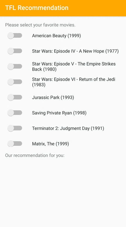
- Question answering app: Given an article and a user question, the model can answer the question within the article.
- Smart reply app: Given previous context, the model can predict and generate potential auto replies.
The pretrained models used in the above reference apps are available in TensorFlow Hub. The chart below shows a comparison of the latency, size and F1 score between the models.
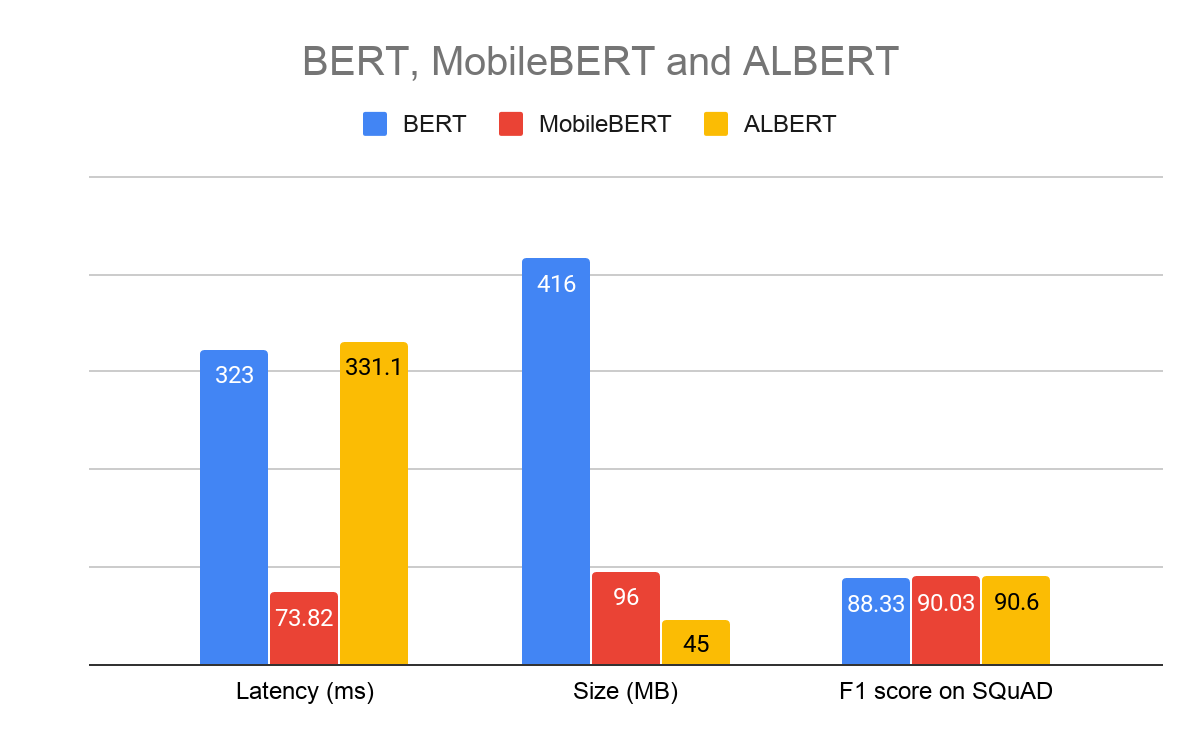 |
| Benchmark on Pixel 4 CPU, 4 Threads, March 2020 Model hyper parameters: Sequence length 128, Vocab size 30K |
Optimizing NLP Models for on-device use cases
On-device models have different constraints compared to server-side models. They run on devices with less memories and slower chips and hence need to be optimized for size and inference speed.Here are several examples of how we optimize models for NLP tasks.
Quantized MobileBERT
MobileBERT is a compact BERT model open sourced on GitHub. It is 4.3x smaller & 5.5x faster than BERT base (float32) while achieving comparable results on GLUE and SQuAD datasets.
After the initial release, we further improved the model by using quantization to optimize its model size and performance, so that it can utilize accelerators like GPU/DSP if available. The quantized MobileBERT is 16x smaller & 8x faster than the BERT base, with little accuracy loss. The MLPerf for Mobile community is leveraging the quantized MobileBERT model for mobile inference benchmarking, and the model can also run in Chrome using TensorFlow.js.
Compared with the original BERT base model (416MB), the below table shows the performance of quantized MobileBERT under the same setting. 
Embedding-free NLP models with projection methods
Language Identification is a type of problems to classify the language of a given text. Recently we open source two models using projection methods, namely SGNN and PRADO.
We used SGNN to show how easy and efficient to use Tensorflow Lite for NLP Tasks. SGNN projects texts to fixed-length features followed by fully connected layers. With annotations to tell TensorFlow Lite converter to fuse TF.Text API, we can get a more efficient model for inference on TensorFlow Lite. Previously, the model took 1332.87 μs to run on benchmark; and after fusion, we see 64.06 μs on the same machine. This brings the magic of 20x speed-up.
We also demonstrate a model architecture called PRADO. PRADO first computes trainable projected features from the sequence of word tokens, then applies convolution and attention to map features to a fixed-length encoding. By combining a projection layer, a convolutional and attention encoder mechanism, PRADO achieves similar accuracy as LSTM, but with 100x smaller model size.
The idea behind these models is to use projection to compute features from texts, so that the model does not need to maintain a big embedding table to convert text features to embeddings. In this way, we’ve proven the model will be much smaller than embedding based models, while maintaining similar performance and inference latency.
Creating your own NLP Models
In addition to using pre-trained models, TensorFlow Lite also provides you with tools such as Model Maker to customize existing models for your own data.
TensorFlow Lite Model Maker: Transfer Learning Toolkit for machine learning beginners
TensorFlow Lite Model Maker is an easy-to-use transfer learning tool to adapt state-of-the-art machine learning models to your dataset. It allows mobile developers to create a model without any machine learning expertise, reduces the required training data and shortens the training time through transfer learning.
After the initial release focusing on vision tasks, we recently added two new NLP tasks to Model Maker. You can follow the colab and guide for Text Classification and Question Answer. To install Model Maker:
pip install tflite-model-makerTo customize the model, developers need to write a few lines of python code as follow:
# Loads Data.
train_data = TextClassifierDataLoader.from_csv(train_csv_file, mode_spec=spec)
test_data = TextClassifierDataLoader.from_csv(test_csv_file, mode_spec=spec)

# Customize the TensorFlow model.
model = text_classifier.create(train_data, model_spec=spec)

# Evaluate the model.
loss, acc = model.evaluate(test_data)

# Export as a TensorFlow Lite model.
model.export(export_dir, quantization_config=config)
Conversion: Better support to convert NLP models to TensorFlow Lite
Since the TensorFlow Lite builtin operator library only supports a subset of TensorFlow operators, you may have run into issues while converting your NLP model to TensorFlow Lite, either due to missing ops or unsupported data types (like RaggedTensor support, hash table support, and asset file handling, etc.). Here are a few tips on how to resolve the conversion issues in such cases.
Run TensorFlow ops and TF.text ops in TensorFlow Lite
We have enhanced Select TensorFlow ops to support various cases. With Select TF ops, developers can leverage TensorFlow ops to run models on TensorFlow Lite, when there are no built-in TensorFlow Lite equivalent ops. For example, it’s common to use TF.Text ops and RaggedTensor when training TensorFlow models, and now those models can be easily converted to TensorFlow Lite and run with necessary ops.
Furthermore, we provide the solution of using op selectively building, so that we get a trimmed binary for mobile deployment. It can select a small set of used ops in the final build target, and thus reduces the binary size in deployment.
More efficient and friendly custom ops
In TensorFlow Lite, we provide a few new mobile-friendly ops for NLP, such as Ngram, SentencePieceTokenizer, WordPieceTokenizer and WhitespaceTokenizer.
Previously, there were several restrictions blocking models with SentencePiece from being converted to TensorFlow Lite. The new SentencePieceTokenizer API for mobile resolves these challenges, and simultaneously optimizes the implementation to make it run faster.
Similarly, Ngram and WhitespaceTokenizer are now not only supported, but will also be executed more efficiently on devices.
TensorFlow Lite recently announced operation fusion with MLIR. We used the same mechanism to fuse TF.Text APIs into custom TensorFlow Lite ops, improving inference efficiency significantly. For example, the WhitespaceTokenizer API was made up of multiple ops, and took 0.9ms to run in the original graph in TensorFlow Lite. After fusing these ops into a single op, it finishes in 0.04ms, a 23x speed-up. This approach has been proven to bring a huge gain in inference latency in the SGNN model mentioned above.
Hash table support
Hash table is important for many NLP models, since we usually need to utilize numeric computation in the language model by transforming words into token IDs and vice versa. Hash table will be enabled in TensorFlow Lite soon. It is supported by handling asset files natively in the TensorFlow Lite format and delivering op kernels as TensorFlow Lite built-in operators.
Deployment: How to run NLP models on-device
Running inference with TensorFlow Lite is now much easier than before. You can use pre-built inference APIs to integrate your model within 5 lines of code, or use utilities to build your own Android/iOS inference APIs.
Simple model deployment using TensorFlow Lite Task Library
The TensorFlow Lite Task Library is a powerful and easy-to-use task-specific library that provides out of the box pre- and post-processing utilities required for ML inference, enabling app developers to easily create machine learning features with TensorFlow Lite. There are three text APIs supported in the Task Library, which correspond to the use cases and models mentioned above:
- NLClassifier: classifies the input text to a set of known categories.
- BertNLClassifier: classifies text optimized for BERT-family models.
- BertQuestionAnswerer: answers questions based on the content of a given passage with BERT-family models.
The Task Library works cross-platform on both Android and iOS. The following example shows inference with a BertQA model in Java/Swift:
// Initialization
BertQuestionAnswerer answerer = BertQuestionAnswerer.createFromFile(androidContext, modelFile);
// Answer a question
List answers = answerer.answer(context, question);| Java code for Android |
// Initialization
let mobileBertAnswerer =   TFLBertQuestionAnswerer.mobilebertQuestionAnswerer(modelPath: modelPath)
// Answer a question
let answers = mobileBertAnswerer.answer(context: context, question: question)| Swift code for iOS |
Customized Inference APIs
If your use case is not supported by the existing task libraries, you can also leverage the Task API Infrastructure and build your own C++/Android/iOS inference APIs using common NLP utilities such as Wordpiece and Sentencepiece tokenizers in the same repo.
Conclusion
In this article, we introduced the new support for NLP tasks in TensorFlow Lite. With the latest update of TensorFlow Lite, developers can easily create, convert and deploy NLP models on-device. We will continue providing more useful tools, and accelerate the development of on-device NLP models from research to production. We would love to hear your feedback, and suggestions for newer NLP tools and utilities. Please email tflite@tensorflow.org or create a TensorFlow Lite support GitHub issue.
Acknowledgments
We like to thank Khanh LeViet, Arun Venkatesan, Max Gubin, Robby Neale, Terry Huang, Peter Young, Gaurav Nemade, Prabhu Kaliamoorthi, Ping Yu, Renjie Liu, Lu Wang, Xunkai Zhang, Yuqi Li, Sijia Ma, Thai Nguyen, Xingying Song, Chung-Ching Chang, Shuangfeng Li to contribute to the blogpost.Read More