 Posted by Ruoxi Wang, Phil Sun, Rakesh Shivanna and Maciej Kula (Google)
In September, we open-sourced TensorFlow Recommenders, a library that makes building state-of-the-art recommender system models easy. Today, we’re excited to announce a new release of TensorFlow Recommenders (TFRS), v0.3.0.
The new version brings two important features, both critical to building and deploying high-quality, scalable recommender models.
The first is built-in support for fast, scalable approximate retrieval. By leveraging ScaNN, TFRS now makes it possible to build deep learning recommender models that can retrieve the best candidates out of millions in milliseconds – all while retaining the simplicity of deploying a single “query features in, recommendations out” SavedModel object.
The second is support for better techniques for modelling feature interactions. The new release of TFRS includes an implementation of Deep & Cross Network: efficient architectures for learning interactions between all the different features used in a deep learning recommender model.
If you’re eager to try out the new features, you can jump straight into our efficient retrieval and feature interaction modelling tutorials. Otherwise, read on to learn more!
Efficient retrieval
The goal of many recommender systems is to retrieve a handful of good recommendations out of a pool of millions or tens of millions of candidates. The retrieval stage of a recommender system tackles the “needle in a haystack” problem of finding a short list of promising candidates out of the entire candidate list.
As discussed in our previous blog post, TensorFlow Recommenders makes it easy to build two-tower retrieval models. Such models perform retrieval in two steps:
- Mapping user input to an embedding
- Finding the top candidates in embedding space
The cost of the first step is largely determined by the complexity of the query tower model. For example, if the user input is text, a query tower that uses an 8-layer transformer will be roughly twice as expensive to compute as one that uses a 4-layer transformer. Techniques such as sparsity, quantization, and architecture optimization all help with reducing this cost.
However, for large databases with millions of candidates, the second step is generally even more important for fast inference. Our two-tower model uses the dot product of the user input and candidate embedding to compute candidate relevancy, and although computing dot products is relatively cheap, computing one for every embedding in a database, which scales linearly with database size, quickly becomes computationally infeasible. A fast nearest neighbor search (NNS) algorithm is therefore crucial for recommender system performance.
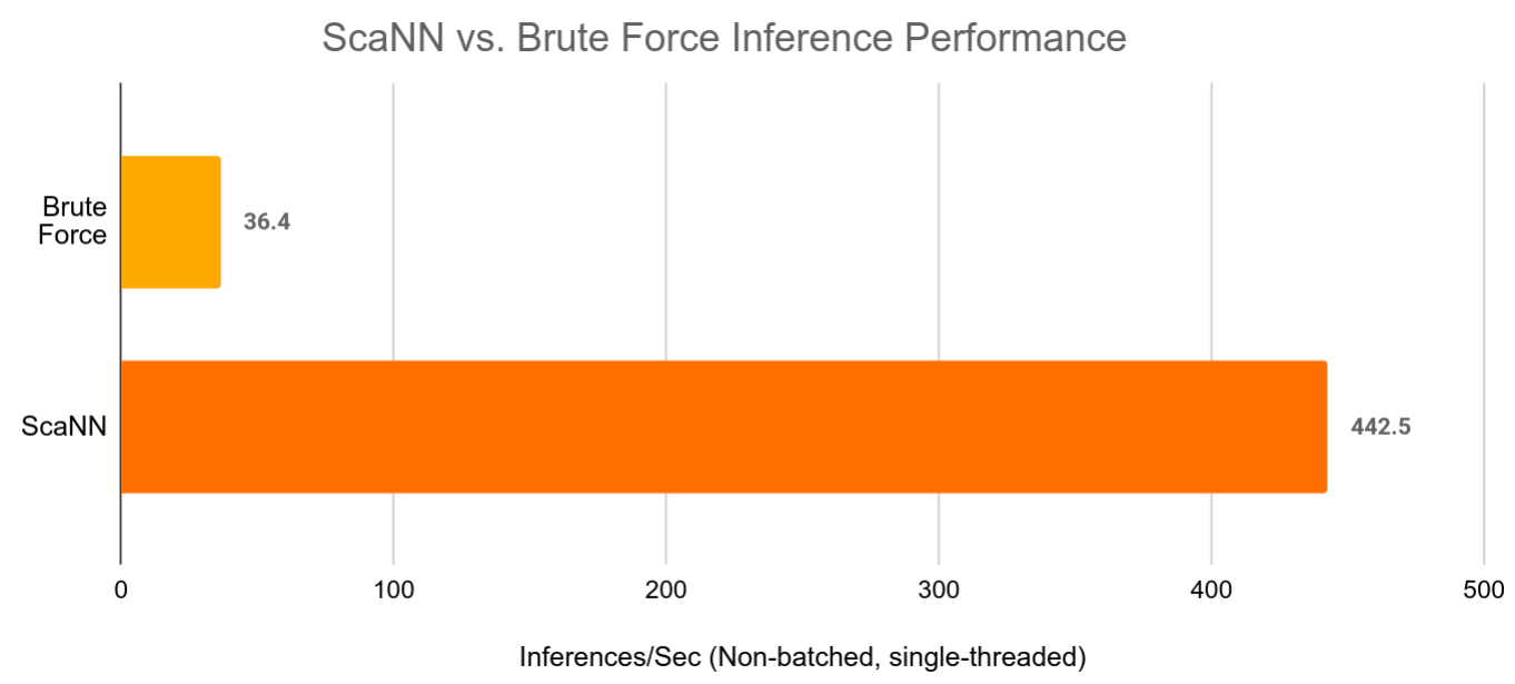
Enter ScaNN. ScaNN is a state-of-the-art NNS library from Google Research. It significantly outperforms other NNS libraries on standard benchmarks. Furthermore, it integrates seamlessly with TensorFlow Recommenders. As seen below, the ScaNN Keras layer acts as a seamless drop-in replacement for brute force retrieval:
# Create a model that takes in raw query features, and
# recommends movies out of the entire movies dataset.
# Before
# index = tfrs.layers.factorized_top_k.BruteForce(model.user_model)
# index.index(movies.batch(100).map(model.movie_model), movies)
# After
scann = tfrs.layers.factorized_top_k.ScaNN(model.user_model)
scann.index(movies.batch(100).map(model.movie_model), movies)

# Get recommendations.
# Before
# _, titles = index(tf.constant(["42"]))
# After
_, titles = scann(tf.constant(["42"]))
print(f"Recommendations for user 42: {titles[0, :3]}")
Because it’s a Keras layer, the ScaNN index serializes and automatically stays in sync with the rest of the TensorFlow Recommender model. There is also no need to shuttle requests back and forth between the model and ScaNN because everything is already wired up properly. As NNS algorithms improve, ScaNN’s efficiency will only improve and further improve retrieval accuracy and latency.
|
| ScaNN can speed up large retrieval models by over 10x while still providing almost the same retrieval accuracy as brute force vector retrieval. |
We believe that ScaNN’s features will lead to a transformational leap in the ease of deploying state-of-the-art deep retrieval models. If you’re interested in the details of how to build and serve ScaNN based models, have a look at our tutorial.
Deep cross networks
Effective feature crosses are the key to the success of many prediction models. Imagine that we are building a recommender system to sell blenders using users’ past purchase history. Individual features such as the number of bananas and cookbooks purchased give us some information about the user’s intent, but it is their combination – having bought both bananas and cookbooks – that gives us the strongest signal of the likelihood that the user will buy a blender. This combination of features is referred to as a feature cross.

In web-scale applications, data are mostly categorical, leading to large and sparse feature space. Identifying effective feature crosses in this setting often requires manual feature engineering or exhaustive search. Traditional feed-forward multilayer perceptron (MLP) models are universal function approximators; however, they cannot efficiently approximate even 2nd or 3rd-order feature crosses as pointed out in the Deep & Cross Network and Latent Cross papers.
What is a Deep & Cross Network (DCN)?
DCN was designed to learn explicit and bounded-degree cross features more effectively. They start with an input layer (typically an embedding layer), followed by a cross network which models explicit feature interactions, and finally a deep network that models implicit feature interactions.
Cross Network
This is the core of a DCN. It explicitly applies feature crossing at each layer, and the highest polynomial degree (feature cross order) increases with layer depth. The following figure shows the (𝑖+1)-th cross layer.
 |
| Cross layer visualization. x0 is the base layer (typically set as the embedding layer), xi is the input to the cross layer, ☉ represents element-wise multiplications, and matrix W and vector b are the parameters to be learned. |
When we only have a single cross layer, it creates 2nd-order (pairwise) feature crosses among input features. In the blender example above, the input to the cross layer would be a vector that concatenates three features: [country, purchased_bananas, purchased_cookbooks]. Then, the first dimension of the output would contain a weighted sum of pairwise interactions between country and all the three input features; the second dimension would contain weighted interactions of purchased_bananas and all the other features, and so on.
The weights of these interaction terms form the matrix W: if an interaction is unimportant, its weight will be close to zero. If it is important, it will be away from zero.
To create higher-order feature crosses, we could stack more cross layers. For example, we now know that a single cross layer outputs 2nd-order feature crosses such as interaction between purchased_bananas and purchased_cookbook. We could further feed these 2nd-order crosses to another cross layer. Then, the feature crossing part would multiply those 2nd-order crosses with the original (1st-order) features to create 3rd-order feature crosses, e.g., interactions among countries, purchased_bananas and purchased_cookbooks. The residual connection would carry over those feature crosses that have already been created in the previous layer.
If we stack k cross layers together, the k-layered cross network would create all the feature crosses up to order k+1, with their importance characterized by parameters in the weight matrices and bias vectors.
Deep Network
The deep part of a Deep & Cross Network is a traditional feedforward multilayer perceptron (MLP).
The deep network and cross network are then combined to form DCN. Commonly, we could stack a deep network on top of the cross network (stacked structure); we could also place them in parallel (parallel structure).
 |
| Deep & Cross Network (DCN) visualization. Left: parallel structure; Right: stacked structure. |
Model Understanding
A good understanding of the learned feature crosses helps improve model understandability. Fortunately, the weight matrix 𝑊 in the cross layer reveals what feature crosses the model has learned to be important.
Take the example of selling a blender to a customer. If purchasing both bananas and cookbooks is the most predictive signal in the data, a DCN model should be able to capture this relationship. The following figure shows the learned matrix of a DCN model with one cross layer, trained on synthetic data where the joint purchase feature is most important. We see that the model itself has learned that the interaction between `purchased_bananas` and `purchased_cookbooks` is important, without any manual feature engineering applied.
 |
| Learned weight matrix in the cross layer. |
Cross layers are now implemented in TensorFlow Recommenders, and you can easily adopt them as building blocks in your models. To learn how, check out our tutorial for example usage and practical lessons. If you are interested in more detail, have a look at our research papers DCN and DCN v2.
Acknowledgements
We would like to give a special thanks to Derek Zhiyuan Cheng, Sagar Jain, Shirley Zhe Chen, Dong Lin, Lichan Hong, Ed H. Chi, Bin Fu, Gang (Thomas) Fu and Mingliang Wang for their critical contributions to Deep & Cross Network (DCN). We also would like to thank everyone who has helped with and supported the DCN effort from research idea to productionization: Shawn Andrews, Sugato Basu, Jakob Bauer, Nick Bridle, Gianni Campion, Jilin Chen, Ting Chen, James Chen, Tianshuo Deng, Evan Ettinger, Eu-Jin Goh, Vidur Goyal, Julian Grady, Gary Holt, Samuel Ieong, Asif Islam, Tom Jablin, Jarrod Kahn, Duo Li, Yang Li, Albert Liang, Wenjing Ma, Aniruddh Nath, Todd Phillips, Ardian Poernomo, Kevin Regan, Olcay Sertel, Anusha Sriraman, Myles Sussman, Zhenyu Tan, Jiaxi Tang, Yayang Tian, Jason Trader, Tatiana Veremeenko, Jingjing Wang, Li Wei, Cliff Young, Shuying Zhang, Jie (Jerry) Zhang, Jinyin Zhang, Zhe Zhao and many more (in alphabetical order). We’d also like to thank David Simcha, Erik Lindgren, Felix Chern, Nathan Cordeiro, Ruiqi Guo, Sanjiv Kumar, Sebastian Claici, and Zonglin Li for their contributions to ScaNN.


 Posted by Karan Shukla, Software Engineer, Google Research

 Posted by Pankaj Kanwar and Fred Alcober


