Posts in category: Tensorflow

Posted by Goldie Gadde and Nikita Namjoshi for the TensorFlow Team

TF 2.4 is here! With increased support for distributed training and mixed precision, new NumPy frontend and tools for monitoring and diagnosing bottlenecks, this release is all about new features and enhancements for performance and scaling.

New Features in tf.distribute

Parameter Server Strategy

In 2.4, the tf.distribute module introduces experimental support for asynchronous training of models with ParameterServerStrategy and custom training loops. Like MultiWorkerMirroredStrategy, ParameterServerStrategy is a multi-worker data parallelism strategy; however, the gradient updates are asynchronous.

A parameter server training cluster consists of workers and parameter servers. Variables are created on parameter servers and then read and updated by workers during each step. The reading and updating of variables happens independently across the workers without any synchronization. Because the workers do not depend on one another, this strategy has the benefit of worker fault tolerance and is useful if you use preemptible VMs.

To get started with this strategy, check out the Parameter Server Training tutorial. This tutorial shows you how to set up ParameterServerStrategy and define a training step, and explains how to use the ClusterCoordinator class to dispatch the execution of training steps to remote workers.

Multi Worker Mirrored Strategy

MultiWorkerMirroredStrategy has moved out of experimental and is now part of the stable API. Like its single worker counterpart, MirroredStrategy, MultiWorkerMirroredStrategy implements distributed training with synchronous data parallelism. However, as the name suggests, with MultiWorkerMirroredStrategy you can train across multiple machines, each with potentially multiple GPUs.

In synchronous training, each worker computes the forward and backward passes on different slices of the input data, and the gradients are aggregated before updating the model. For this aggregation, known as an all-reduce, MultiWorkerMirroredStrategy uses CollectiveOps to keep variables in sync. A collective op is a single op in the TensorFlow graph that can automatically choose an all-reduce algorithm in the TensorFlow runtime according to hardware, network topology, and tensor sizes.

To get started with MultiWorkerMirroredStrategy, check out the Multi-worker training with Keras tutorial, which has been updated with details on dataset sharding, saving/loading models trained with a distribution strategy, and failure recovery with the BackupAndRestore callback.

If you are new to distributed training and want to learn how to get started, or you’re interested in distributed training on GCP, see this blog post for an introduction to the key concepts and steps.

Updates in Keras

Mixed Precision

In TensorFlow 2.4, the Keras mixed precision API has moved out of experimental and is now a stable API. Most TensorFlow models use the float32 dtype; however, there are lower-precision types such as float16 that use less memory. Mixed precision is the use of 16-bit and 32-bit floating point types in the same model for faster training. This API can improve model performance by 3x on GPUs and 60% on TPUs.

To make use of the mixed precision API, you must use Keras layers and optimizers, but it’s not necessary to use other Keras classes such as models or losses. If you’re curious to learn how to take advantage of this API for better performance, check out the Mixed Precision tutorial.

Optimizers

This release includes refactoring the tf.keras.optimizers.Optimizer class, enabling users of model.fit or custom training loops to write training code that works with any optimizer. All built-in tf.keras.optimizer.Optimizer subclasses now accept gradient_transformers and gradient_aggregator arguments, allowing you to easily define custom gradient transformations.

With the refactor, you can now pass a loss tensor directly to Optimizer.minimize when writing custom training loops:

tape = tf.GradientTape()
with tape:
  y_pred = model(x, training=True)
  loss = loss_fn(y_pred, y_true)

# You can pass in the `tf.GradientTape` when using a loss `Tensor` as shown below.

optimizer.minimize(loss, model.trainable_variables, tape=tape)

These changes are intended to make both Model.fit and custom training loops more agnostic to optimizer details, allowing you to write training code that works with any optimizer without modification.

Functional API model construction internal improvements

Lastly, TensorFlow 2.4 includes a major refactoring of the internals of the Keras Functional API, improving the memory consumption of functional model construction and simplifying triggering logic. This refactoring also ensures TensorFlowOpLayers behave predictably and work with CompositeTensor type signatures.

Introducing tf.experimental.numpy

TensorFlow 2.4 introduces experimental support for a subset of NumPy APIs, available as tf.experimental.numpy. This module enables you to run NumPy code, accelerated by TensorFlow. Because it is built on top of TensorFlow, this API interoperates seamlessly with TensorFlow, allowing access to all of TensorFlow’s APIs and providing optimized execution using compilation and auto-vectorization. For example, TensorFlow ND arrays can interoperate with NumPy functions, and similarly TensorFlow NumPy functions can accept inputs of different types including tf.Tensor and np.ndarray.

import tensorflow.experimental.numpy as tnp

# Use NumPy code in input pipelines

dataset = tf.data.Dataset.from_tensor_slices(
    tnp.random.randn(1000, 1024)).map(
    lambda z: z.clip(-1,1)).batch(100)

# Compute gradients through NumPy code

def grad(x, wt):
  with tf.GradientTape() as tape:
    tape.watch(wt)
    output = tnp.dot(x, wt)
    output = tf.sigmoid(output)
  return tape.gradient(tnp.sum(output), wt)

You can learn more about how to use this API in the NumPy API on TensorFlow guide.

New Profiler Tools

MultiWorker Support in TensorFlow Profiler

The TensorFlow Profiler is a suite of tools you can use to measure the training performance and resource consumption of your TensorFlow models. The TensorFlow Profiler helps you understand the hardware resource consumption of the ops in your model, diagnose bottlenecks, and ultimately train faster.

Previously, the TensorFlow Profiler supported monitoring multi-GPU, single host training jobs. In 2.4 you can now profile MultiWorkerMirroredStrategy training jobs. For example, you can use the sampling mode API to perform on demand profiling and connect to the same server:port in use by MultiWorkerMirroredStrategy workers:

# Start a profiler server before your model runs.


tf.profiler.experimental.server.start(6009)

# Model code goes here....
 
# E.g. your worker IP addresses are 10.0.0.2, 10.0.0.3, 10.0.0.4, and you
# would like to profile for a duration of 2 seconds. The profiling data will
# be saved to the Google Cloud Storage path “your_tb_logdir”.
 
tf.profiler.experimental.client.trace(
    'grpc://10.0.0.2:6009,grpc://10.0.0.3:6009,grpc://10.0.0.4:6009',
    'gs://your_tb_logdir',
    2000)

Alternatively, you can use the TensorBoard profile plugin by providing the worker addresses to the Capture Profile tool.

After profiling, you can use the new Pod Viewer tool to choose a training step and view its step-time category breakdown across all workers.

For more information on how to use the TensorFlow Profiler, check out the newly released GPU Performance Guide. This guide shows common scenarios you might encounter when you profile your model training job and provides a debugging workflow to help you get better performance, whether you’re training with one GPU, multiple GPUs, or multiple machines.

TFLite Profiler

The TFLite Profiler enables tracing TFLite internals in Android to identify performance bottlenecks. The TFLite Performance Measurement Guide shows you how to add trace events, enable TFLite tracing, and capture traces with both the Android Studio CPU Profiler and the System Tracing app.

Example trace using the Android System Tracing app

New Features for GPU Support

TensorFlow 2.4 runs with CUDA 11 and cuDNN 8, enabling support for the newly available NVIDIA Ampere GPU architecture. To learn more about CUDA 11 features, check out this NVIDIA developer blog.

Additionally, support for TensorFloat-32 on Ampere-based GPUs is enabled by default. TensorFloat-32, or `TF32` for short, is a math mode for NVIDIA Ampere GPUs that causes certain float32 ops, such as matrix multiplications and convolutions, to run much faster on Ampere GPUs but with reduced precision. To learn more , see the documentation for tf.config.experimental.enable_tensor_float_32_execution.

Next steps

Check out the release notes for more information. To stay up to date, you can read the TensorFlow blog, follow twitter.com/tensorflow, or subscribe to youtube.com/tensorflow. If you’ve built something you’d like to share, please submit it for our Community Spotlight at goo.gle/TFCS. For feedback, please file an issue on GitHub. Thank you!

Read More

Posted by Arno Eigenwillig, Software Engineer and Luiz GUStavo Martins, Developer Advocate

BERT and other Transformer encoder architectures have been very successful in natural language processing (NLP) for computing vector-space representations of text, both in advancing the state of the art in academic benchmarks as well as in large-scale applications like Google Search. BERT has been available for TensorFlow since it was created, but originally relied on non-TensorFlow Python code to transform raw text into model inputs.

Today, we are excited to announce a more streamlined approach to using BERT built entirely in TensorFlow. This solution makes both pre-trained encoders and the matching text preprocessing models available on TensorFlow Hub. BERT in TensorFlow can now be run on text inputs with just a few lines of code:

# Load BERT and the preprocessing model from TF Hub.
preprocess = hub.load('https://tfhub.dev/tensorflow/bert_en_uncased_preprocess/1')
encoder = hub.load('https://tfhub.dev/tensorflow/bert_en_uncased_L-12_H-768_A-12/3')

# Use BERT on a batch of raw text inputs.
input = preprocess(['Batch of inputs', 'TF Hub makes BERT easy!', 'More text.'])
pooled_output = encoder(input)["pooled_output"]
print(pooled_output)

tf.Tensor(
[[-0.8384154  -0.26902363 -0.3839138  ... -0.3949695  -0.58442086  0.8058556 ]
 [-0.8223734  -0.2883956  -0.09359277 ... -0.13833837 -0.6251748   0.88950026]
 [-0.9045408  -0.37877116 -0.7714909  ... -0.5112085  -0.70791864  0.92950743]],
shape=(3, 768), dtype=float32)

These encoder and preprocessing models have been built with TensorFlow Model Garden’s NLP library and exported to TensorFlow Hub in the SavedModel format. Under the hood, preprocessing uses TensorFlow ops from the TF.text library to do the tokenization of input text – allowing you to build your own TensorFlow model that goes from raw text inputs to prediction outputs without Python in the loop. This accelerates the computation, removes boilerplate code, is less error prone, and enables the serialization of the full text-to-outputs model, making BERT easier to serve in production.

To show in more detail how these models can help you, we’ve published two new tutorials:

• The beginner tutorial solves a sentiment analysis task and doesn’t need any special customization to achieve great model quality. It’s the easiest way of using BERT and a preprocessing model.
• The advanced tutorial solves NLP classification tasks from the GLUE benchmark, running on TPU. It also shows how to use the preprocessing model in situations where you need multi-segment input.

Choosing a BERT model

BERT models are pre-trained on a large corpus of text (for example, an archive of Wikipedia articles) using self-supervised tasks like predicting words in a sentence from the surrounding context. This type of training allows the model to learn a powerful representation of the semantics of the text without needing labeled data. However, it also takes a significant amount of computation to train – 4 days on 16 TPUs (as reported in the 2018 BERT paper). Fortunately, after this expensive pre-training has been done once, we can efficiently reuse this rich representation for many different tasks.

TensorFlow Hub offers a variety of BERT and BERT-like models:

• Eight BERT models come with the trained weights released by the original BERT authors.
• 24 Small BERTs have the same general architecture but fewer and/or smaller Transformer blocks, which lets you explore tradeoffs between speed, size and quality.
• ALBERT: these are four different sizes of “A Lite BERT” that reduces model size (but not computation time) by sharing parameters between layers.
• The 8 BERT Experts all have the same BERT architecture and size but offer a choice of different pre-training domains and intermediate fine-tuning tasks, to align more closely with the target task.
• Electra has the same architecture as BERT (in three different sizes), but gets pre-trained as a discriminator in a set-up that resembles a Generative Adversarial Network (GAN).
• BERT with Talking-Heads Attention and Gated GELU [base, large] has two improvements to the core of the Transformer architecture.
• Lambert has been trained with the LAMB optimizer and several techniques from RoBERTa.
• … and more to come.

These models are BERT encoders. The links above take you to their documentation on TF Hub, which refers to the right preprocessing model for use with each of them.

We encourage developers to visit these model pages to learn more about the different applications targeted by each model. Thanks to their common interface, it’s easy to experiment and compare the performance of different encoders on your specific task by changing the URLs of the encoder model and its preprocessing.

The Preprocessing model

For each BERT encoder, there is a matching preprocessing model. It transforms raw text to the numeric input tensors expected by the encoder, using TensorFlow ops provided by the TF.text library. Unlike preprocessing with pure Python, these ops can become part of a TensorFlow model for serving directly from text inputs. Each preprocessing model from TF Hub is already configured with a vocabulary and its associated text normalization logic and needs no further set-up.

We’ve already seen the simplest way of using the preprocessing model above. Let’s look again more closely:

preprocess = hub.load('https://tfhub.dev/tensorflow/bert_en_uncased_preprocess/1')
input = preprocess(["This is an amazing movie!"])
 
{'input_word_ids': <tf.Tensor: shape=(1, 128), dtype=int32, numpy=
  array([[ 101, 2023, 2003, 2019, 6429, 3185,  999,  102,    0,  ...]])>,
 'input_mask': <tf.Tensor: shape=(1, 128), dtype=int32, numpy=
  array([[   1,    1,    1,    1,    1,    1,    1,    1,    0,  ...,]])>,
 'input_type_ids': <tf.Tensor: shape=(1, 128), dtype=int32, numpy=
  array([[   0,    0,    0,    0,    0,    0,    0,    0,    0,  ...,]])>}
 

Calling preprocess() like this transforms raw text inputs into a fixed-length input sequence for the BERT encoder. You can see that it consists of a tensor input_word_ids with numerical ids for each tokenized input, including start, end and padding tokens, plus two auxiliary tensors: an input_mask (that tells non-padding from padding tokens) and input_type_ids for each token (that can distinguish multiple text segments per input, which we will discuss below).

The same preprocessing SavedModel also offers a second, more fine-grained API, which supports putting one or two distinct text segments into one input sequence for the encoder. Let’s look at a sentence entailment task, in which BERT is used to predict if a premise entails a hypothesis or not:

text_premises = ["The fox jumped over the lazy dog.",
                 "Good day."]
tokenized_premises = preprocess.tokenize(text_premises)
 
<tf.RaggedTensor
  [[[1996], [4419], [5598], [2058], [1996], [13971], [3899], [1012]],
  [[2204], [2154], [1012]]]>
 
 
text_hypotheses = ["The dog was lazy.",  # Entailed.
                   "Axe handle!"]        # Not entailed.
tokenized_hypotheses = preprocess.tokenize(text_hypotheses)
 
<tf.RaggedTensor
  [[[1996], [3899], [2001], [13971], [1012]],
  [[12946], [5047], [999]]]>

The result of each tokenization is a RaggedTensor of numeric token ids, representing each of the text inputs in full. If some pairs of premise and hypothesis are too long to fit within the seq_length for BERT inputs in the next step, you can do additional preprocessing here, such as trimming the text segment or splitting it into multiple encoder inputs.

The tokenized input then gets packed into a fixed-length input sequence for the BERT encoder:

encoder_inputs = preprocess.bert_pack_inputs(
   [tokenized_premises, tokenized_hypotheses],
   seq_length=18)  # Optional argument, defaults to 128.
 
{'input_word_ids': <tf.Tensor: shape=(2, 18), dtype=int32, numpy=
  array([[  101,  1996,  4419,  5598,  2058,  1996, 13971,  3899,  1012,
            102,  1996,  3899,  2001, 13971,  1012,   102,     0,     0],
         [  101,  2204,  2154,  1012,   102, 12946,  5047,   999,   102,
              0,     0,     0,     0,     0,     0,     0,     0,     0]])>,
 'input_mask': <tf.Tensor: shape=(2, 18), dtype=int32, numpy=
  array([[1, 1, 1, 1, 1, 1, 1, 1, 1, 1, 1, 1, 1, 1, 1, 1, 0, 0],
         [1, 1, 1, 1, 1, 1, 1, 1, 1, 0, 0, 0, 0, 0, 0, 0, 0, 0]])>,
 'input_type_ids': <tf.Tensor: shape=(2, 18), dtype=int32, numpy=
  array([[0, 0, 0, 0, 0, 0, 0, 0, 0, 0, 1, 1, 1, 1, 1, 1, 0, 0],
         [0, 0, 0, 0, 0, 1, 1, 1, 1, 0, 0, 0, 0, 0, 0, 0, 0, 0]])>}

The result of packing is the already-familiar dict of input_word_ids, input_mask and input_type_ids (which are 0 and 1 for the first and second input, respectively). All outputs have a common seq_length (128 by default). Inputs that would exceed seq_length are truncated to approximately equal sizes during packing.

Accelerating model training

TensorFlow Hub provides BERT encoder and preprocessing models as separate pieces to enable accelerated training, especially on TPUs.

Tensor Processing Units (TPUs) are Google’s custom-developed accelerator hardware that excel at large scale machine learning computations such as those required to fine-tune BERT. TPUs operate on dense Tensors and expect that variable-length data like strings has already been transformed into fixed-size Tensors by the host CPU.

The split between the BERT encoder model and its associated preprocessing model enables distributing the encoder fine-tuning computation to TPUs as part of model training, while the preprocessing model executes on the host CPU. The preprocessing computation can be run asynchronously on a dataset using tf.data.Dataset.map() with dense outputs ready to be consumed by the encoder model on the TPU. Asynchronous preprocessing like this can improve performance with other accelerators as well.

Our advanced BERT tutorial can be run in a Colab runtime that uses a TPU worker and demonstrates this end-to-end.

Summary

Using BERT and similar models in TensorFlow has just gotten simpler. TensorFlow Hub makes available a large collection of pre-trained BERT encoders and text preprocessing models that are easy to use in just a few lines of code.

Take a look at our interactive beginner and advanced tutorials to learn more about how to use the models for sentence and sentence-pair classification. Let us know what you build with these new BERT models and tag your posts with #TFHub.

Acknowledgements:

We’d like to thank a number of colleagues for their contribution to this work.

The new preprocessing models have been created in collaboration with Chen Chen, Terry Huang, Mark Omernick and Rajagopal Ananthanarayanan.

Additional BERT models have been published to TF Hub on this occasion by Sebastian Ebert (Small BERTs), Le Hou and Hongkun Yu (Lambert, Talking Heads).

Mark Daoust, Josh Gordon and Elizabeth Kemp have greatly improved the presentation of the material in this post and the associated tutorials.

Read More

Posted by Amy Hsueh, TensorFlow Partnerships Lead, and Sandeep Gupta, TensorFlow Product Manager

Implementing machine learning solutions can help businesses innovate, but it can be a challenge if companies don’t have the knowledge, experience, or resources in-house to get started.

That’s where our TensorFlow AI Service Partners may be able to help. We’ve selected AI/ML practitioners who have experience helping businesses implement AI/ML and TensorFlow-based solutions. We hope that these partners can help more enterprises benefit from AI-based systems and innovate faster, solve smarter, and scale bigger.

“Service partners are critical in driving large adoption of AI in the enterprise”, said Kemal El Moujahid, Director of Product Management for TensorFlow, “so we are excited to partner with some of the leading AI Service companies, who excel at building powerful solutions with TensorFlow. The breadth and diversity of business problems that these companies solve for their customers are incredible, and we are looking forward to seeing even more real-world impact with TensorFlow.”

Our selected partners are experienced in creating a range of consulting and software solutions powered by TensorFlow and other frameworks that span across the machine learning workflow, including preparing and ingesting data, training and optimizing models, and productionizing them.

TensorFlow AI Service Partners share their insights and product feedback with the TensorFlow team, helping us make enhancements and improvements that address enterprise ML needs.

“We are thrilled to be partnering with companies that have deep TensorFlow expertise and demonstrated track records in solving their customer’s business critical needs,” remarks Sarah Sirajuddin, Engineering Director of TensorFlow, “We value user feedback tremendously, and believe that the feedback and insights gathered from these partners will help us improve TensorFlow for all our users.”

Choose from our partners, ranging in geographic reach and industry specializations, all with demonstrated expertise in TensorFlow on our website or hear from them directly on why they are excited about this program on their respective blogs: Determined AI, Labelbox, Paperspace, SpringML, Stradigi AI, Quantiphi.

We look forward to seeing this program grow and adding additional partners in the future. If you’re interested in becoming a partner, check out our application guide.

Read More

Posted by Nikita Namjoshi, Machine Learning Solutions Engineer

For many in the world of data science, distributed training can seem a daunting task. In addition to building and thoughtfully evaluating a high-quality ML model, you have to be aware of how to optimize your model for specific hardware and manage infrastructure. The latter skills are not often included in a data scientist’s toolkit. However, with the help of managed services on the Google Cloud Platform (GCP), you can easily scale your model training job to multiple accelerators or even multiple machines, with no GPU expertise required.

In this tutorial-style article, you’ll get hands-on experience with GCP data science tools and train a TensorFlow model across multiple GPUs. You’ll also learn key terminology in the field of distributed training, such as data parallelism, synchronous training, and AllReduce.

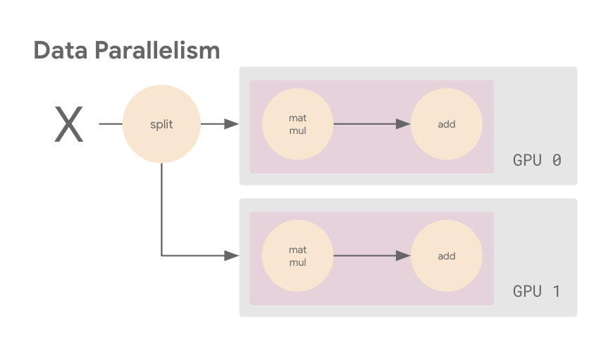
Data parallelism is one of the concepts you will learn about in this article.

Why Distributed Training?

Every data scientist and machine learning engineer has experienced the agony of sitting and waiting for a model to train. Even if you have access to a GPU, with a large dataset it can take days for a large deep learning model to converge. Using the right hardware configuration can reduce training time to hours, or even minutes. And a shorter training time makes for faster iteration to reach your modeling goals.

If you have a GPU available, TensorFlow will use it automatically with no code changes required. Similarly, TensorFlow can make use of multiple CPU cores out of the box. However, if you want to train with two or more GPUs then you’ll have to do a bit of extra work. This extra work is necessary because TensorFlow needs to know how to coordinate the training process across the multiple GPUs in your runtime. Fortunately, with the tf.distribute module, you have access to different distributed training strategies that you can easily incorporate into your program.

When doing distributed training, it’s important to be clear on the distinction between machines and devices. A device refers to a CPU or accelerator, such as GPUs or TPUs, on some machine that TensorFlow can run operations on. The focus in this article will be training with a single machine that has multiple GPU devices, but the tf.distribute.Strategy API also provides support for multi-worker training. In a multi-worker set up, the training is distributed across multiple machines. These machines can be CPU only, or have one or more GPU devices each.

Single GPU Training

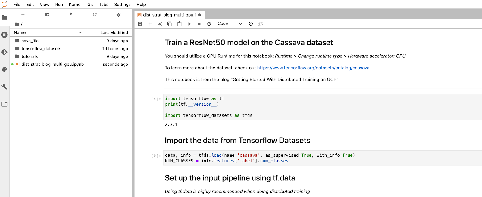
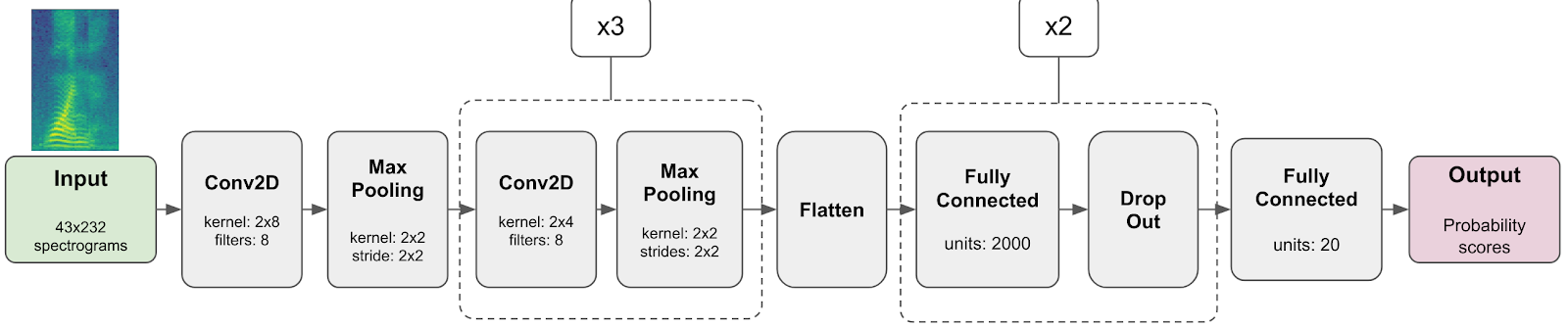
In the following Colab notebook, you’ll find the code to train a ResNet50 architecture on the Cassava dataset. If you execute the cells in the notebook and train the model, you’ll notice that the number of steps taken in each epoch is 89, and each epoch takes around 100 seconds. Make note of these numbers; we will come back to them later.

Multi-GPU Training

You can access a single GPU in colab, but your luck stops there if you want to use multiple GPUs. Moreover, while a Colab notebook is great for quick experimentation you’ll likely want a more secure and reliable set up that offers you more control over your environment. For that, you can turn to the cloud.

There are many different ways to do distributed training on GCP. Picking the best option for your use case will likely involve different considerations if you are a student/researcher running experiments, versus an engineer at a company training models in a production workflow.

In this article you will use the GCP AI Platform Notebooks. This path provides an easy approach to distributed training and also gives you a chance to explore a managed notebook environment running on GCP. As an alternative, if you already have a local environment set up and are looking for a hassle free transition between your local and GCP environments, you can check out the TensorFlow Cloud library. TensorFlow Cloud can automate many of the steps described in this article; however, we will walk through the steps here so you can get a deeper understanding of the key concepts involved in distributed training.

In the following section, you’ll learn how to modify the single GPU training code using the tf.distribute.Strategy API. The resulting code will be cloud platform agnostic so you could run it in a different environment without any changes. You can also run the same code on your own hardware.

Prepare Code for Distributed Training

The first step in using the tf.distribute.Strategy API is to instantiate your strategy. In this tutorial, you will use MirroredStrategy, which is one of several distribution strategies available in TensorFlow.

strategy = tf.distribute.MirroredStrategy()

Next, you need to wrap the creation of your model parameters within the scope of the strategy. This step is crucial because it tells MirroredStrategy which variables to mirror across your GPU devices.

with strategy.scope():
   model = create_model()
   model.compile(
     loss='sparse_categorical_crossentropy',
     optimizer=tf.keras.optimizers.Adam(0.0001),
     metrics=['accuracy'])

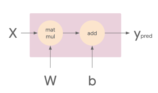
Before we run the updated code, let’s take a brief look at what will actually happen when we call model.fit and how training will differ now that we have added a strategy. For the sake of simplicity, imagine you have a simple linear model instead of the ResNet50 architecture. In TensorFlow, you can think of this simple model in terms of its computational graph.

In the image below, you can see that the matmul op takes in the X and W tensors, which are the training batch and weights respectively. The resulting tensor is then passed to the add op with the tensor b, which is the model’s bias terms. The result of this op is Y_pred, which is the model’s predictions.

We want a way of executing this computational graph such that we can leverage two GPUs. There are multiple different ways we can achieve this. For example, you could put different layers of your model on different machines or devices, which is one flavor of model parallelism. Alternatively, you could distribute your dataset such that each device processes a portion of the input batch on each training step with the same model, which is known as data parallelism. Or you might do a combination of both. Data parallelism is the most common (and easiest) approach, and that’s what we’ll do here.

The next image shows an example of data parallelism. The input batch X is split in half, and one slice is sent to GPU 0 and the other to GPU 1. In this case, each GPU calculates the same ops but on different slices of the data.

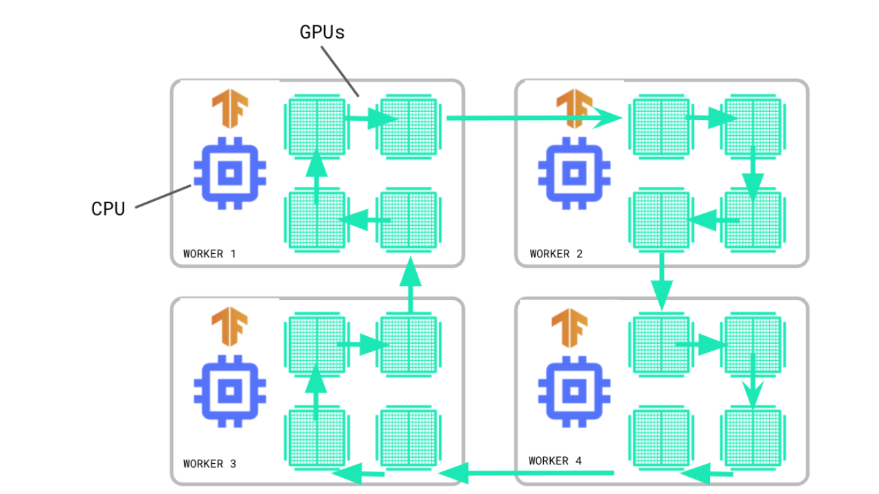
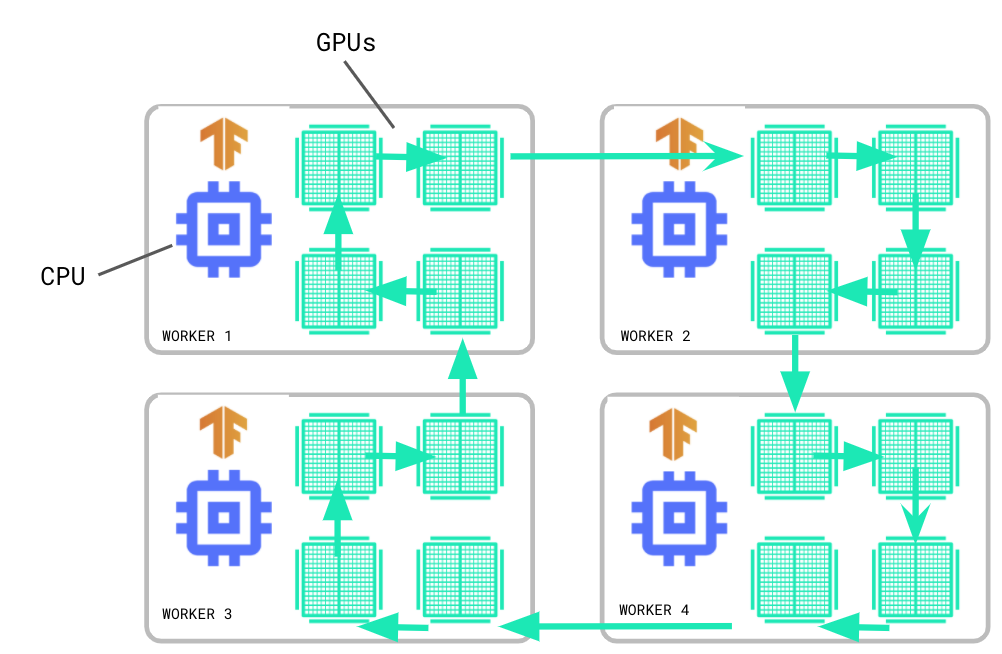
MirroredStrategy is a data parallelism strategy. So when we call model.fit, MirroredStrategy will make a copy (known as a replica) of the ResNet50 model on both of the GPUs. The CPU (host) is responsible for preparing the tf.data.Dataset batches and sending the data to the GPUs (devices).

The subsequent gradient updates will happen in a synchronous manner. This means that each worker device computes the forward and backward passes through the model on a different slice of the input data. The computed gradients from each of these slices are then aggregated across all of the devices and reduced (usually an average) in a process known as AllReduce. The optimizer then performs the parameter updates with these reduced gradients thereby keeping the devices in sync. Because each worker cannot proceed to the next training step until all the other workers have finished the current step, this gradient calculation becomes the main overhead in distributed training for synchronous strategies.

While MirroredStrategy is a synchronous strategy, data parallelism strategies can also be asynchronous. In an asynchronous data parallelism strategy, each worker computes the gradients from a slice of the input data and makes updates to the parameters in an asynchronous fashion. Compared to synchronous strategies, asynchronous training has the benefit of fault tolerance because the workers are not dependent on one another, but can result in stale gradients. You can learn more about asynchronous training by experimenting with the TensorFlow Parameter Server Strategy.

With the two easy steps of instantiating MirroredStrategy, and then wrapping your model creation within the strategy scope, TensorFlow will do the heavy lifting of distributing your training job across your GPUs through data parallelism and synchronous gradient updates.

The last change you will want to make is to the batch size.

BATCH_SIZE = 64 * strategy.num_replicas_in_sync

Recall that in the single GPU case, the batch size was 64. This means that on each step of model training, 64 images were processed, and the number of resulting steps in each epoch was the total dataset size / batch size, which we noted previously as 89.

When you do distributed training with the tf.distribute.Strategy API and tf.data, the batch size now refers to the global batch size. In other words, if you pass a batch size of 10, and you have two GPUs, then each machine will process 5 examples per step. In this case, 10 is known as the global batch size, and 5 as the per replica batch size. To make the most out of your GPUs, you will want to scale the batch size by the number of replicas, which is two in this case because there is one replica on each GPU.

You can make these code changes yourself, or simply use this other Colab notebook where the changes have been made already. Although MirroredStrategy is designed for a multi-GPU environment, you can actually run this notebook in Colab on a GPU runtime or a CPU runtime without error. TensorFlow will use a single GPU or multiple CPU cores out of the box anyway so you don’t actually need a strategy, but this could come in handy for testing/experimentation purposes.

Set up GCP Project

Now that we’ve made the necessary code changes, the next step is to set up the GCP environment. To do this you will need a GCP project with billing enabled.

1. Create your project in the UI
2. Create your billing account

Next, you should enable the Cloud Compute Engine API. If you are working in a brand new project, then this process will likely also prompt you to connect the billing account you created. If you are using a GCP project that you have already worked with, then most likely the Compute Engine API will already be enabled.

Request Quota

Google Cloud enforces quotas on resource usage to prevent abuse and accidental usage. If you need access to more of a particular resource than what is available by default, you’ll have to request more quota. For this tutorial, we will use the NVIDIA T4 GPU. By default, you get access to one T4 GPU per location, but in order to do distributed training you’ll need to request quota for an additional GPU in a location.

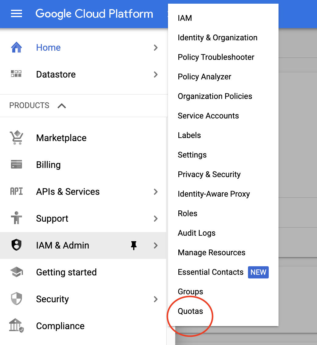
In the GCP console, scroll to the hamburger menu on the left side and navigate to IAM & Admin > Quotas

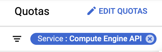
On the Quotas page you can add a service filter for the Compute Engine API. Note that if you have not enabled the Compute Engine API or enabled billing, you will not see Compute Engine API as a filter option, so be sure you have completed the earlier steps first.

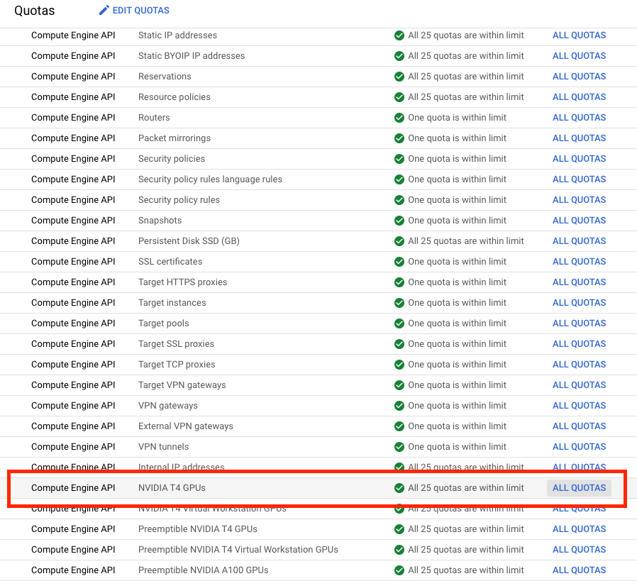
When you find the NVIDIA T4 GPU resource in the list, go ahead and click on ALL QUOTAS for that row.

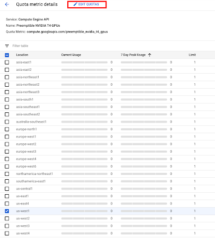
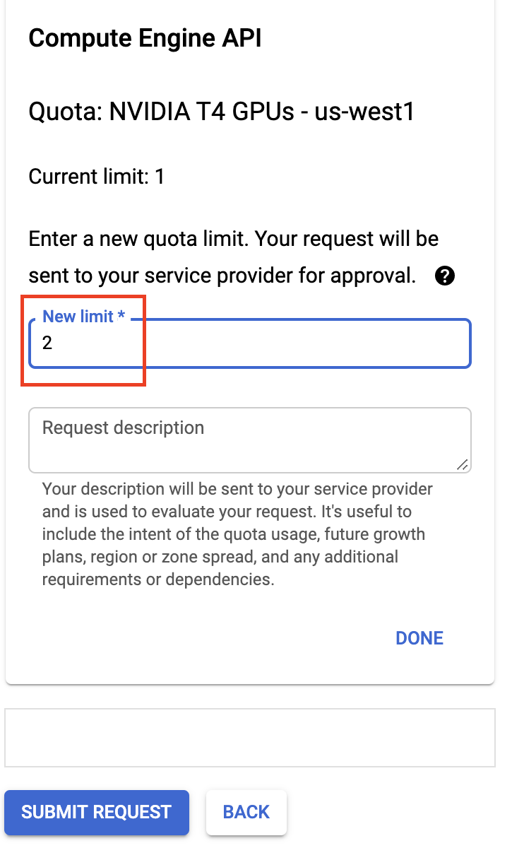
Once you’ve made it to the Quota metric details page for NVIDIA T4 GPUs, select the Location: us-west1 and click edit quotas at the top of the page.

If you already have quota for a different type of GPU, or in a different location, you can easily use those instead. Just make sure you remember the GPU type and location as you will need to specify these parameters when setting up your AI Platform Notebook environment later. Additionally, if you prefer to follow along and just use a single GPU instead of requesting quota for two, you can do that as well. Your code will not be distributed, but you will still get the benefit of learning how to set your GCP environment.

>

Fill in your contact details in the Quota changes menu and then set your New Limit to 2. Then click Done when you’re finished.

You’ll get a confirmation email first when you have submitted the request, and then when your request has been approved.

Create AI Platform Notebook Instance

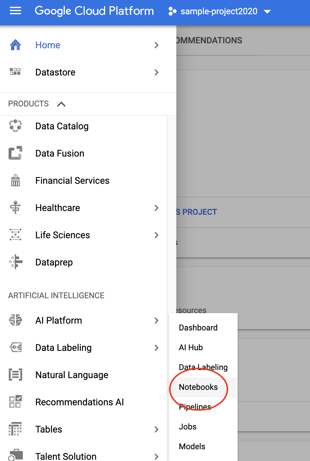
While you wait for quota approvals, the next step is to get set up with AI Platform Notebooks, which can be found using the same hamburger menu as before in the console and scrolling to Artificial Intelligence > AI Platform > Notebooks

You’ll need to enable the API if this is your first time using the tool.

AI Platform Notebooks is a managed service for doing data science work. This tool is ideal if you like developing in a notebook environment. You can easily add and remove GPUs without having to worry about GPU driver installation, and there are a number of instance images you can choose from depending on your use case so you don’t need to hassle with setting up all the Python packages you need to get your job done.

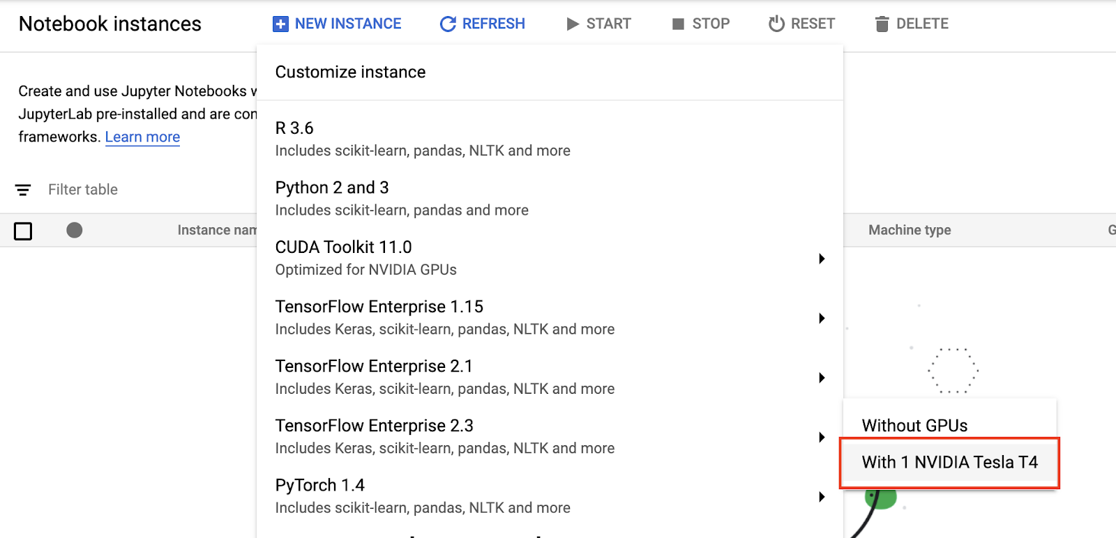
Once the Notebooks API is enabled, the next step is to create your instance. You can do this by clicking the NEW INSTANCE button at the top of the page, and then selecting the TensorFlow Enterprise 2.3 image (or the most recent TensorFlow image if you’re following along at a later date), with the 1 NVIDIA Tesla T4 option. TensorFlow Enterprise is a TensorFlow distribution optimized for GCP.

Click ADVANCED OPTIONS at the bottom of the New notebook instance window, and then change the following fields:

• Instance name: give your instance a name
• Region: us-west1
• GPU type: NVIDIA Tesla T4
• Number of GPUs: 2
• Check the Install NVIDIA GPU driver automatically for me box

Then click CREATE. Note that if you have not yet been approved for the NVIDIA T4 quota, you will get an error message when you click CREATE. So be sure you have received your approval message before completing this step. Additionally, if you plan to use a different GPU type or location other than T4 in us-west1, you will need to change these parameters when creating your notebook.

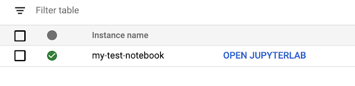
Your instance will take a few minutes to launch, and when it’s done you’ll see the option to OPEN JUPYTERLAB appear in blue letters.

Note that even after you’ve created an AI Platform Notebook instance, you can change the hardware (for example adding or removing GPUs). Should you need to do this in the future, simply stop the instance and follow the steps here.

Train Multi-GPU Model on AI Platform Notebooks

Now that your instance is set up, you can click on OPEN JUPYTERLAB.

Download the Colab Notebook as an .ipynb file, and upload it to your Jupyter Lab environment. When the file is uploaded go to the notebook and run the code.

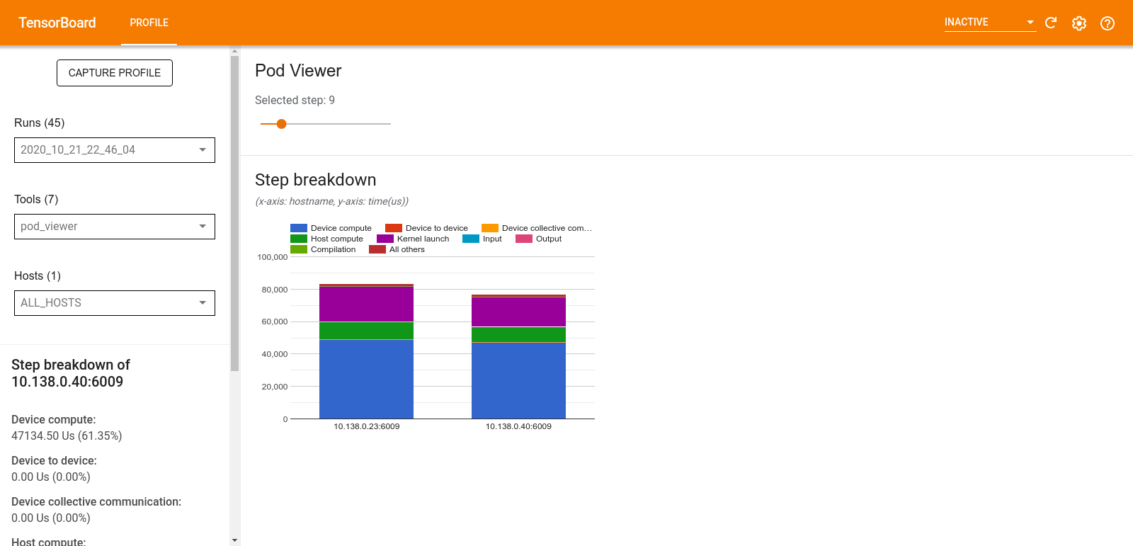
When you execute the model.fit cell, you should notice that the number of steps per epoch is now 45, which is half of what it was when using a single GPU. This is data parallelism in action. With a global batch size of 64 * 2, your CPU is sending batches of 64 images to each GPU. So while previously the model only saw 64 examples in a single step, it now sees 128 examples on each step and thus each epoch takes less time. Previously each epoch took around 100 seconds, and now each epoch takes around 60 seconds. You’ll notice that adding a second GPU does not cut the time in half, as there is some overhead involved in synchronizing the gradients. The benefits will be more noticeable with a larger dataset (Cassava only has 5656 training images). Additionally, there are lots of techniques you can use to get even more benefit from that second GPU, such as making sure your input pipeline isn’t a bottleneck. To learn more about making the most of your GPUs, see the TensorFlow Performance Debugging guide.

Long Running Jobs on the DLVM

So far you’ve learned how to use the GCP AI Platform Notebooks to run a simple distributed training job. The dataset we used was not very large, and the model achieved fairly high accuracy after only a few epochs. However, in reality your training job will probably run for a lot longer and you might not want to use a notebook.

When you launch an AI Platform Notebook, it creates a Google Compute Engine (GCE) instance using the GCP Deep Learning VM Images. The Deep Learning VM images are Compute Engine virtual machine images optimized for data science and machine learning tasks. In our example we used the TensorFlow Enterprise 2.3 image, but there are many other options available.

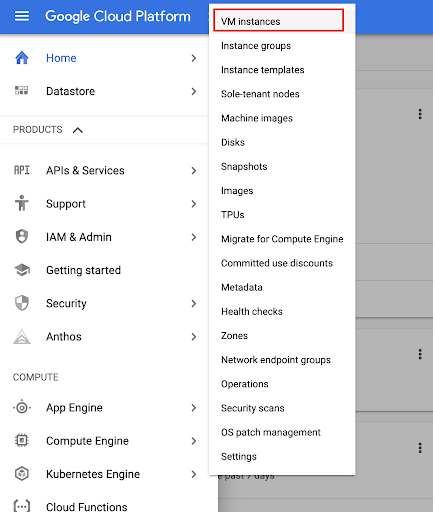
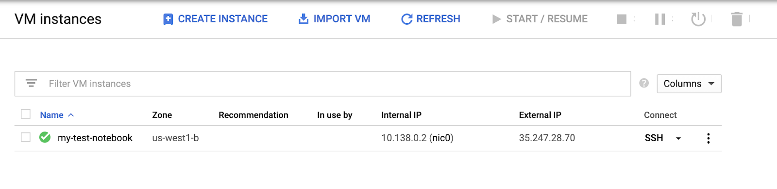
In the console, you can use the menu to navigate to Compute Engine > VM instances

And you should see an instance with the same name as the notebook you created earlier. Because this is a GCE instance, we can ssh into the machine and run the code there.

Install Google SDK

Installing the Google Cloud SDK will allow you to manage GCE resources in your project from your terminal. Follow the steps here to install the SDK and connect to your project.

SSH into the VM

Once the SDK is installed and configured, you can use the following command in your terminal to ssh into your vm. Just be sure to change the instance name and project name.

gcloud compute ssh {your-vm-name} --project={your-project-name}

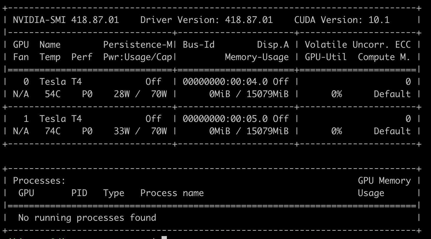
If you run the command nvidia-smi on the vm, you’ll see the two T4 GPUs we provisioned earlier.

To run the distributed training job, simply download the code from the Colab Notebook as a .py file, and use the following command from your local machine to copy it to your vm.

gcloud compute scp --project {your-project-name} {local-path-to-py-file} {your-vm-name}:~/

Finally, you can run the script on your vm with

python dist_strat_blog_multi_gpu.py

And you should see the output of your model training job

If Notebooks are your environment of choice, you can stick with the workflow we used in the previous section. But if you prefer to use vim or emacs, or if you want to run a long running job using Screen for example, you have the option to ssh into the vm from your terminal. Note that you can also launch a Deep Learning VM directly from the command line instead of using the AI Platform Notebooks UI like we did in this tutorial.

When you’re finished experimenting, do not forget to shut your instance down. You can do this by selecting the instance from the Notebook instances page, or GCE Instances page in the console UI and clicking STOP at the top of the window. Shutting down the instance is very important as you will be billed a few dollars for every hour that it is left running. You can easily stop your instance, then restart it when you want to run more experiments and all of your files will still be there.

Take Your Distributed Training Skills to the Next Level

In this article you learned how to use MirroredStrategy, a synchronous data parallelism strategy, to distribute your TensorFlow training job across two GPUs on GCP. You now know the basic mechanics of how to set up your GCP environment and prepare your code, but there’s a lot more to explore in the world of distributed training. For example, if you are interested in building a distributed training job into a production ML pipeline, check out the AI Platform Training Service, which also allows you to configure a training job across multiple machines, each containing multiple GPUs.

On the tensorflow.org site you can check out the other strategies available with the tf.distribute.Strategy API in the overview guide, and also learn how to use a strategy with a custom training loop. For more advanced concepts, there’s a guide on how data gets distributed, and a guide on how to do performance debugging with the TensorFlow Profiler to make sure you are maximizing utilization of your GPUs.

Read More

Posted by Khanh LeViet, TensorFlow Developer Advocate

Sound classification is a machine learning task where you input some sound to a machine learning model to categorize it into predefined categories such as dog barking, car horn and so on. There are already many applications of sound classification, including detecting illegal deforestation activities, or detecting sound of humpback whales for better understanding about their natural behaviors.

We are excited to announce that Teachable Machine now allows you to train your own sound classification model and export it in the TensorFlow Lite (TFLite) format. Then you can integrate the TFLite model to your mobile applications or your IoT devices. This is an easy way to quickly get up and running with sound classification, and you can then explore building production models in Python and exporting them to TFLite as a next step.

Model architecture

The model that Teachable Machine uses to classify 1-second audio samples is a small convolutional neural network. As the diagram above illustrates, the model receives a spectrogram (2D time-frequency representation of sound obtained through Fourier transform). It first processes the spectrogram with successive layers of 2D convolution (Conv2D) and max pooling layers. The model ends in a number of dense (fully-connected) layers, which are interleaved with dropout layers for the purpose of reducing overfitting during training. The final output of the model is an array of probability scores, one for each class of sound the model is trained to recognize.

You can find a tutorial to train your own sound classifications models using this approach in Python here.

Train a model using your own dataset

There are two ways to train a sound classification model using your own dataset:

• Simple way: Use Teachable Machine to collect training data and train the model all within your browser without writing a single line of code. This approach is useful for those who want to build a prototype quickly and interactively.
• Robust way: Record sounds to use as your training dataset in advance then use Python to train and carefully evaluate your model. Of course, his approach is also more automated and repeatable than the simple way.

Train a model using Teachable Machine

Teachable Machine is a GUI tool that allows you to create training dataset and train several types of machine learning models, including image classification, pose classification and sound classification. Teachable Machine uses TensorFlow.js under the hood to train your machine learning model. You can export the trained models in TensorFlow.js format to use in web browsers, or export in TensorFlow Lite format to use in mobile applications or IoT devices.

Here are the steps to train your models:

1. Go to Teachable Machine website
2. Create an audio project
3. Record some sound clips for each category that you want to recognize. You need only 8 seconds of sound for each category.
4. Start training. Once it has finished, you can test your model on live audio feed.
5. Export the model in TFLite format.

Train a model using Python

If you have a large training dataset with several hours of sound recording and or than a dozen of categories, then training a sound classification on a web browser will likely take a lot of time. In that case, you can collect the training dataset in advance, convert them to the WAV format and use this Colab notebook (which includes steps to convert the model to TFLite format) to train your sound classification. Google Colab offers a free GPU so that you can significantly speed up your model training.

Deploy the model to Android with TensorFlow Lite

Once you have trained your TensorFlow Lite sound classification model, you can just put it in this Android sample app to try it out. Just follow these steps:

1. Clone the sample app from GitHub:
   git clone https://github.com/tensorflow/examples.git
2. Import the sound classification Android app into Android Studio. You can find it in the lite/examples/sound_classification/android folder.
3. Add your model (both the soundclassifier.tflite and labels.txt) into the src/main/assets folder replacing the example model that is already there.
4. Build the app and deploy it on an Android device. Now you can classify sound in real time!

To integrate the model into your own app, you can copy the SoundClassifier.kt class from the sample app and the TFLite model you have trained to your app. Then you can use the model as below:

1. Initialize a `SoundClassifier` instance from your `Activity` or `Fragment` class.

var soundClassifier: SoundClassifier
soundClassifier = SoundClassifier(context).also {
    it.lifecycleOwner = context
}

2. Start capturing live audio from the device’s microphone and classify in real time:

soundClassifier.start()

3. Receive classification results in real time as a map of human-readable class names and probabilities of the current sound belonging to each particular category.

let labelName = soundClassifier.labelList[0] // e.g. "Clap"
soundClassifier.probabilities.observe(this) { resultMap ->
    let probability = result[labelName] // e.g. 0.7
}

What’s next

We are working on an iOS version of the sample app that will be released in a few weeks. We will also extend TensorFlow Lite Model Maker to allow easy training of sound classification in Python. Stay tuned!

Acknowledgements

This project is a joint effort between multiple teams inside Google. Special thanks to:

• Google Research: Shanqing Cai, Lisie Lillianfeld
• TensorFlow team: Tian Lin
• Teachable Machine team: Gautam Bose, Jonas Jongejan
• Android team: Saryong Kang, Daniel Galpin, Jean-Michel Trivi, Don Turner

Read More

Posted by Ruoxi Wang, Phil Sun, Rakesh Shivanna and Maciej Kula (Google)

In September, we open-sourced TensorFlow Recommenders, a library that makes building state-of-the-art recommender system models easy. Today, we’re excited to announce a new release of TensorFlow Recommenders (TFRS), v0.3.0.

The new version brings two important features, both critical to building and deploying high-quality, scalable recommender models.

The first is built-in support for fast, scalable approximate retrieval. By leveraging ScaNN, TFRS now makes it possible to build deep learning recommender models that can retrieve the best candidates out of millions in milliseconds – all while retaining the simplicity of deploying a single “query features in, recommendations out” SavedModel object.

The second is support for better techniques for modelling feature interactions. The new release of TFRS includes an implementation of Deep & Cross Network: efficient architectures for learning interactions between all the different features used in a deep learning recommender model.

If you’re eager to try out the new features, you can jump straight into our efficient retrieval and feature interaction modelling tutorials. Otherwise, read on to learn more!

Efficient retrieval

The goal of many recommender systems is to retrieve a handful of good recommendations out of a pool of millions or tens of millions of candidates. The retrieval stage of a recommender system tackles the “needle in a haystack” problem of finding a short list of promising candidates out of the entire candidate list.

As discussed in our previous blog post, TensorFlow Recommenders makes it easy to build two-tower retrieval models. Such models perform retrieval in two steps:

1. Mapping user input to an embedding
2. Finding the top candidates in embedding space

The cost of the first step is largely determined by the complexity of the query tower model. For example, if the user input is text, a query tower that uses an 8-layer transformer will be roughly twice as expensive to compute as one that uses a 4-layer transformer. Techniques such as sparsity, quantization, and architecture optimization all help with reducing this cost.

However, for large databases with millions of candidates, the second step is generally even more important for fast inference. Our two-tower model uses the dot product of the user input and candidate embedding to compute candidate relevancy, and although computing dot products is relatively cheap, computing one for every embedding in a database, which scales linearly with database size, quickly becomes computationally infeasible. A fast nearest neighbor search (NNS) algorithm is therefore crucial for recommender system performance.

Enter ScaNN. ScaNN is a state-of-the-art NNS library from Google Research. It significantly outperforms other NNS libraries on standard benchmarks. Furthermore, it integrates seamlessly with TensorFlow Recommenders. As seen below, the ScaNN Keras layer acts as a seamless drop-in replacement for brute force retrieval:

# Create a model that takes in raw query features, and
# recommends movies out of the entire movies dataset.
# Before
# index = tfrs.layers.factorized_top_k.BruteForce(model.user_model)
# index.index(movies.batch(100).map(model.movie_model), movies)
# After
scann = tfrs.layers.factorized_top_k.ScaNN(model.user_model)
scann.index(movies.batch(100).map(model.movie_model), movies)

# Get recommendations.
# Before
# _, titles = index(tf.constant(["42"]))
# After
_, titles = scann(tf.constant(["42"]))
print(f"Recommendations for user 42: {titles[0, :3]}")

Because it’s a Keras layer, the ScaNN index serializes and automatically stays in sync with the rest of the TensorFlow Recommender model. There is also no need to shuttle requests back and forth between the model and ScaNN because everything is already wired up properly. As NNS algorithms improve, ScaNN’s efficiency will only improve and further improve retrieval accuracy and latency.

ScaNN can speed up large retrieval models by over 10x while still providing almost the same retrieval accuracy as brute force vector retrieval.

We believe that ScaNN’s features will lead to a transformational leap in the ease of deploying state-of-the-art deep retrieval models. If you’re interested in the details of how to build and serve ScaNN based models, have a look at our tutorial.

Deep cross networks

Effective feature crosses are the key to the success of many prediction models. Imagine that we are building a recommender system to sell blenders using users’ past purchase history. Individual features such as the number of bananas and cookbooks purchased give us some information about the user’s intent, but it is their combination – having bought both bananas and cookbooks – that gives us the strongest signal of the likelihood that the user will buy a blender. This combination of features is referred to as a feature cross.

In web-scale applications, data are mostly categorical, leading to large and sparse feature space. Identifying effective feature crosses in this setting often requires manual feature engineering or exhaustive search. Traditional feed-forward multilayer perceptron (MLP) models are universal function approximators; however, they cannot efficiently approximate even 2nd or 3rd-order feature crosses as pointed out in the Deep & Cross Network and Latent Cross papers.

What is a Deep & Cross Network (DCN)?

DCN was designed to learn explicit and bounded-degree cross features more effectively. They start with an input layer (typically an embedding layer), followed by a cross network which models explicit feature interactions, and finally a deep network that models implicit feature interactions.

Cross Network

This is the core of a DCN. It explicitly applies feature crossing at each layer, and the highest polynomial degree (feature cross order) increases with layer depth. The following figure shows the (𝑖+1)-th cross layer.

Cross layer visualization. x0 is the base layer (typically set as the embedding layer), xi is the input to the cross layer, ☉ represents element-wise multiplications, and matrix W and vector b are the parameters to be learned.

When we only have a single cross layer, it creates 2nd-order (pairwise) feature crosses among input features. In the blender example above, the input to the cross layer would be a vector that concatenates three features: [country, purchased_bananas, purchased_cookbooks]. Then, the first dimension of the output would contain a weighted sum of pairwise interactions between country and all the three input features; the second dimension would contain weighted interactions of purchased_bananas and all the other features, and so on.

The weights of these interaction terms form the matrix W: if an interaction is unimportant, its weight will be close to zero. If it is important, it will be away from zero.

To create higher-order feature crosses, we could stack more cross layers. For example, we now know that a single cross layer outputs 2nd-order feature crosses such as interaction between purchased_bananas and purchased_cookbook. We could further feed these 2nd-order crosses to another cross layer. Then, the feature crossing part would multiply those 2nd-order crosses with the original (1st-order) features to create 3rd-order feature crosses, e.g., interactions among countries, purchased_bananas and purchased_cookbooks. The residual connection would carry over those feature crosses that have already been created in the previous layer.

If we stack k cross layers together, the k-layered cross network would create all the feature crosses up to order k+1, with their importance characterized by parameters in the weight matrices and bias vectors.

Deep Network

The deep part of a Deep & Cross Network is a traditional feedforward multilayer perceptron (MLP).

The deep network and cross network are then combined to form DCN. Commonly, we could stack a deep network on top of the cross network (stacked structure); we could also place them in parallel (parallel structure).

Deep & Cross Network (DCN) visualization. Left: parallel structure; Right: stacked structure.

Model Understanding

A good understanding of the learned feature crosses helps improve model understandability. Fortunately, the weight matrix 𝑊 in the cross layer reveals what feature crosses the model has learned to be important.

Take the example of selling a blender to a customer. If purchasing both bananas and cookbooks is the most predictive signal in the data, a DCN model should be able to capture this relationship. The following figure shows the learned matrix of a DCN model with one cross layer, trained on synthetic data where the joint purchase feature is most important. We see that the model itself has learned that the interaction between `purchased_bananas` and `purchased_cookbooks` is important, without any manual feature engineering applied.

Learned weight matrix in the cross layer.

Cross layers are now implemented in TensorFlow Recommenders, and you can easily adopt them as building blocks in your models. To learn how, check out our tutorial for example usage and practical lessons. If you are interested in more detail, have a look at our research papers DCN and DCN v2.

Acknowledgements

We would like to give a special thanks to Derek Zhiyuan Cheng, Sagar Jain, Shirley Zhe Chen, Dong Lin, Lichan Hong, Ed H. Chi, Bin Fu, Gang (Thomas) Fu and Mingliang Wang for their critical contributions to Deep & Cross Network (DCN). We also would like to thank everyone who has helped with and supported the DCN effort from research idea to productionization: Shawn Andrews, Sugato Basu, Jakob Bauer, Nick Bridle, Gianni Campion, Jilin Chen, Ting Chen, James Chen, Tianshuo Deng, Evan Ettinger, Eu-Jin Goh, Vidur Goyal, Julian Grady, Gary Holt, Samuel Ieong, Asif Islam, Tom Jablin, Jarrod Kahn, Duo Li, Yang Li, Albert Liang, Wenjing Ma, Aniruddh Nath, Todd Phillips, Ardian Poernomo, Kevin Regan, Olcay Sertel, Anusha Sriraman, Myles Sussman, Zhenyu Tan, Jiaxi Tang, Yayang Tian, Jason Trader, Tatiana Veremeenko‎, Jingjing Wang, Li Wei, Cliff Young, Shuying Zhang, Jie (Jerry) Zhang, Jinyin Zhang, Zhe Zhao and many more (in alphabetical order). We’d also like to thank David Simcha, Erik Lindgren, Felix Chern, Nathan Cordeiro, Ruiqi Guo, Sanjiv Kumar, Sebastian Claici, and Zonglin Li for their contributions to ScaNN.

Read More

A guest post by Owen Lockwood, Rensselaer Polytechnic Institute

Quantum mechanics was once a very controversial theory. Early detractors such as Albert Einstein famously said of quantum mechanics that “God does not play dice” (referring to the probabilistic nature of quantum measurements), to which Niels Bohr replied, “Einstein, stop telling God what to do”. However, all agreed that, to quote John Wheeler “If you are not completely confused by quantum mechanics, you do not understand it”. As our understanding of quantum mechanics has grown, not only has it led to numerous important physical discoveries but it also resulted in the field of quantum computing. Quantum computing is a different paradigm of computing from classical computing. It relies on and exploits the principles of quantum mechanics to achieve speedups (in some cases superpolynomial) over classical computers.

In this article I will be discussing some of the challenges I faced as a beginning researcher in quantum machine learning (QML) and how TensowFlow Quantum (TFQ) and Cirq enabled me and can help other researchers investigate the field of quantum computing and QML. I have previous experience with TensorFlow, which made the transition to using TensorFlow Quantum seamless. TFQ proved instrumental in enabling my work and ultimately my work utilizing TFQ culminated in my first publication on quantum reinforcement learning in the 16th AIIDE conference. I hope that this article helps and inspires other researchers, neophytes and experts alike, to leverage TFQ to help advance the field of QML.

QML Background

QML has important similarities and differences to traditional neural network/deep learning approaches to machine learning. Both methodologies can be seen as using “stacked layers” of transformations that make up a larger model. In both cases, data is used to inform updates to model parameters, typically to minimize some loss function (usually, but not exclusively via gradient based methods). Where they differ is QML models have access to the power of quantum mechanics and deep neural networks do not. An important type of QML that TFQ provides techniques for is called variational quantum circuits (QVC). QVCs are also called quantum neural networks (QNN).

A QVC can be visualized below (from the TFQ white paper). The diagram is read from left to right, with the qubits being represented by the horizontal lines. In a QVC there are three important and distinct parts: the encoder circuit, the variational circuit and the measurement operators. The encoder circuit either takes naturally quantum data (i.e. a nonparametrized quantum circuit) or converts classical data into quantum data. This circuit is connected to the variational circuit which is defined by its learnable parameters. The parametrized part of the circuit is the part that is updated during the learning process. The last part of the QVC is the measurement operators. In order to extract information from the QVC some sort of quantum measurement (such as a Pauli X, Y, or Z basis measurements) must be applied. With the information extracted from these measurements a loss function (and gradients) can be calculated on a classical computer and the parameters can be updated. These gradients can be optimized with the same optimizers as traditional neural networks such as Adam or RMSProp. QVC’s can also be combined with traditional neural networks (as is shown in the diagram) as the quantum circuit is differentiable and thus gradients can be backpropagated through.

However, the intuitive models and mathematical framework surrounding QVCs have some important differences from traditional neural networks, and in these differences lies the potential for quantum speedups. Quantum computing and QML can harness quantum phenomena, such as superposition and entanglement. Superposition stems from the wavefunction being a linear combination of multiple states and enables a qubit to represent two different states simultaneously (in a probabilistic manner). The ability to operate on these superpositions, i.e. operate on multiple states simultaneously, is integral to the power of quantum computing. Entanglement is a complex phenomenon that is induced via multi-qubit gates. Getting a basic understanding of these concepts and of quantum computing is an important first step for QML. There are a number of great resources available for this such as Preskill’s Quantum Computing Course, and de Wolf’s lecture notes.

Currently, access to real quantum hardware is limited and as such, many quantum computing researchers conduct work on simulations of quantum computers. Near term and current quantum devices have 10s-100s of quantum bits (qubits) like the Google sycamore processor. Because of their size and the noise, this hardware is often called Noisy Intermediate Scale Quantum (NISQ) technology. TFQ and Cirq are built for these near term NISQ devices. These devices are far smaller than what some of the most famous quantum algorithms require to achieve quantum speedups given current error correction techniques; e.g. Shor’s algorithm requires upwards of thousands of qubits and the Quantum Approximate Optimization Algorithm (QAOA) could require at least 420 qubits for quantum advantages. However, there is still significant potential for NISQ devices to achieve quantum speedups (as Google demonstrated with 53 qubits).

My Work With TFQ

TFQ was announced in mid March this year (2020) and I began to use it shortly after. Around that time I had begun research into QML, specifically QML for reinforcement learning (RL). While there have been great strides in the accessibility of quantum circuit simulators, QML can be a difficult field to get into. Not only are there difficulties from a mathematical and physical perspective, but the time investment for implementation can be substantial. The time it would take to code QVCs from scratch and properly test and debug them (not to mention the optimization) is a challenge, especially for those coming from classical machine learning. Spending so much time building something for an experiment that has the potential to not work is a big risk – especially for an undergraduate student on a deadline! Thankfully I did not have to take this risk. With the release of TFQ it was easy to immediately start on the implementations of my ideas. Realistically, I would never have done this work if TFQ had not been released. Inspired by previous work, we expanded upon applying QML to RL tasks.

In our work we demonstrate the potential to use QVCs in place of neural networks in contemporary RL algorithms (specifically DQN and DDQN). We also show the potential to use multiple types of QVC models, using QVCs with either a dense layer or quantum pooling layers (denoted hybrid and pure respectively) to shrink the number of qubits to the correct output space.

The representational power of QVCs is also put on display; using a QVC with ~50 parameters we were able to achieve comparable performance to neural networks with orders of magnitude more parameters. See the graphs for a comparison of the reward achieved on the canonical CartPole environment (balancing a pole on a cart), the left graph includes all neural networks and the right shows only the largest neural network. The number in front of the NN represents the size of the parameter space.

We are continuing to work with QML applications to RL and have more manuscripts in submission. Continuation of this work has been accepted into the 2020 NeurIPS workshop: “The pre-registration experiment: an alternative publication model for machine learning research”.

Suggested use of TFQ

TFQ can be an incredible tool for anyone interested in QML research no matter your background. All too common in scientific communities is a ‘publish or perish’ mentality which can stifle innovative work and is prohibitive to intellectual risk taking, especially for experiments that require significant implementation efforts. Not only can TFQ help speed up any experiments you may have, but it also allows for easy implementation of ideas that would otherwise never get tested. Implementation is a common hindrance to new and interesting ideas, and far too many projects never progress out of the idea stage due to difficulties in transitioning the idea to reality, something TFQ makes easy.

For beginners, TFQ enables a first foray into the field without substantial time investment in coding and allows for significant learning. Being able to try and experiment with QVCs without having to build from the ground up is an incredible tool. For classical ML researchers with experience in TensorFlow, TFQ makes it easy to transition and experiment with QML at small or large scales. The API of TFQ and the modules it provides (i.e. Keras-esque layers and differentiators) share design principles with TF and their similarities make for an easier programming transition. For researchers already in the QML field, TFQ can certainly help.

In order to get started with TFQ it is important to become familiar with the basics of quantum computing, with either the references mentioned above or with any of the many other great resources out there. Another important step that often gets overlooked, is reading the TFQ white paper. The white paper is accessible to QML beginners and is an invaluable introduction to QML and the basic as well as advanced usage of TFQ. Just as important is to play around with TFQ. Try different things out, experiment; it is a great way to expand not only understanding of the software but of the theory and mathematics as well. Reading other contemporary papers and the papers that cite TFQ is a great way to become immersed with the current research going on in the field.

Read More

Posted by Siddhant Agarwal and Biswajeet Mallik, Program Managers

TensorFlow has a strong developer community in India with 13 TensorFlow User Groups and 20+ Google Developer Experts. In September, these groups came together to organise the “TFUG India Summit“, a 4-day online event with four tracks. You can check out the recordings for these talks below.

• TensorFlow Core and TensorFlow for Web
• TensorFlow for Mobile
• TensorFlow for Production
• TensorFlow for Research
  

  Thank you to the 14 community leaders from 13 India TFUGs, as well as our GDEs, who organized this event.

  

  How to get involved

  If you would like to start a TFUG in your region, please visit this page. To find a user group near you, check out this list. And, if you have any questions regarding TFUG, email us. Thank you!

Read More

Posted by Jason Mayes, Developer Relations Engineer for TensorFlow.js

The TensorFlow YouTube channel has a new show called “TensorFlow.js Community Show & Tell.” In this program, we highlight amazing tech demos from the TensorFlow.js community every quarter. Our next show will be on 11th December 9AM PT over on the TensorFlow YouTube channel, but if you missed the previous ones, you can find past episodes on this playlist.

About the show

Do you love great tech demos that push the boundaries of what is possible for a given industry? If that sounds like you and you’re looking for fresh inspiration, along with insights from the engineers themselves, then this may be the YouTube show for you.

After hacking with many wonderful folk in the TensorFlow.js community it became clear to us that the creativity and the work you were producing was simply incredible. For that reason, we have put together a brand new format, known as the TensorFlow Show & Tell to showcase top projects that are being made and give developers a platform to share their work. With many subscribers who are as passionate about machine learning as we are, we figured this was a great way to do that and connect great minds.

If you missed our latest show you can check our most recent broadcast here:

We have seen a whole bunch of amazing demos on the first 3 shows using machine learning in truly novel ways. From making music from thin air using your hands which is then web connected to a Tesla coil (yes, that actually happened), to combining machine learning models with mind blowing mixed reality and 3D graphics, we have had a good variety of presenters from all around the world.

Who has presented so far?

We’ve had 25 presenters, and there are more in the making!

1st Show: Rogerio Chaves (Netherlands), Max Bittker (USA), Junya Ishihara (Japan), Ben Farrell (USA), Lizzie Siegle (USA), Manish Raj (India), Yiwen Lin (UK), Jimmy (Thailand)

2nd Show: Cyril Diagne (France), John Cohn (USA), Va Barbosa (USA), FollowTheDarkside (Japan), Jaume Sanchez (UK), Olesya Chernyavskaya (Russia), Alexandre Devaux (France), Amruta (India), Shan Huan (China).

3rd Show: Gant Laborde (USA), Hugo Zanini (Brazil), Charlie Gerard (Amsterdam), Shivay Lamba (India), Anders Jessen (Denmark), Benson Ruan (Australia), Cristina Maillo (Spain), James Seo (USA).

How can I get on the show?

If you have made something using TensorFlow.js simply use the #MadeWithTFJS hashtag over on Twitter or LinkedIn with a post demonstrating your creation and link to try it out. We will select our top picks each quarter to be featured in the show and reach out to you directly if you are selected. You can view existing submissions for Twitter as an example.

I missed an episode – where can I view them?

Catch up on previous live episodes via this playlist, and if you wish to watch shorter bite sized videos over a coffee break you can do so with the Made With TensorFlow.js playlist to allow you to watch just the ones that are relevant to you on demand.

When is the next show?

Join us in December for the next show and tell – we have 6 wonderful new demos lined up. We’re aiming for 11th December, 9AM PT, over on the TensorFlow YouTube channel.

Be sure to subscribe and click the bell icon to set notifications for when new videos are posted (we are aiming for every quarter), or add a Google calendar reminder and see you there!

Also, if you enjoyed the show and would like to see this format replicated for TensorFlow Core, TensorFlow Lite, and more, let us know! You can drop me a message on Twitter or LinkedIn – would love to see what you have made.

Acknowledgements

A huge thank you to all 24 of our show & tell presenters thus far, and to the amazing community who have submitted projects or helped tag amazing finds for us to reach out to. You truly make this show what it is and we are super excited to see even more in the future and look forward to seeing you all again soon.

Read More

Posted by Karan Shukla, Software Engineer, Google Research

Machine learning (ML) model transparency is important across a wide variety of domains that impact peoples’ lives, from healthcare to personal finance to employment. At Google, this desire for transparency led us to develop Model Cards, a framework for transparent reporting on ML model performance, provenance, ethical considerations and more. It can be time consuming, however, to compile the information necessary to create a useful Model Card. To address this, we recently announced the open-source launch of Model Card Toolkit (MCT), a collection of tools that supports ML developers in compiling the information that goes into a Model Card.

The toolkit consists of:

• A JSON schema, which specifies the fields to include in the Model Card
• A ModelCard data API to represent an instance of the JSON schema and visualize it as a Model Card
• A component that uses the model provenance information stored with ML Metadata (MLMD) to automatically populate the JSON with relevant information

We wanted the toolkit to be modular so that Model Card creators can still leverage the JSON schema and ModelCard data API even if their modeling environment is not integrated with MLMD. In this post, we’ll show you how you can use these components to create a Model Card for a Keras MobileNetV2 model trained on ImageNet and fine-tuned on the cats_vs_dogs dataset available in TensorFlow Datasets (TFDS). While this model and use case may be trivial from a transparency standpoint, it allows us to easily demonstrate the components of MCT.

An example Model Card. Click here for a larger version.

Model Card Toolkit Walkthrough

You can follow along and run the code yourself in the Colab notebook. In this walkthrough, we’ll include some additional information about the considerations you’ll want to keep in mind while using the toolkit.

We begin by installing the Model Card Toolkit.

!pip install 'model-card-toolkit>=0.1.1,

Now, we load both the MobileNetV2 model and the weights generated by fine-tuning the model on the cats_vs_dogs dataset. For more information on how we fine-tuned our model, you can see the TensorFlow tutorial on the topic.

URL = 'https://storage.googleapis.com/cats_vs_dogs_model/cats_vs_dogs_model.zip'
BASE_PATH = tempfile.mkdtemp()
ZIP_PATH = os.path.join(BASE_PATH, 'cats_vs_dogs_model.zip')
MODEL_PATH = os.path.join(BASE_PATH,'cats_vs_dogs_model')  
 
r = requests.get(URL, allow_redirects=True)
open(ZIP_PATH, 'wb').write(r.content)
 
with zipfile.ZipFile(ZIP_PATH, 'r') as zip_ref:
    zip_ref.extractall(BASE_PATH)
 
model = tf.keras.models.load_model(MODEL_PATH)

We also calculate the number of examples, storing it to the “examples” object, and the accuracy scores, disaggregated across class. We’ll use both accuracy and examples later to build graphs to display in our Model Card.

examples = cats_vs_dogs.get_data()
accuracy = compute_accuracy(examples['combined'])
cat_accuracy = compute_accuracy(examples['cat'])
dog_accuracy = compute_accuracy(examples['dog'])

Next, we’ll use the Model Card Toolkit to create our Model Card. The first step is to initialize a ModelCardToolkit object, which maintains assets including a Model Card JSON file and Model Card document. Call ModelCardToolkit.scaffold_assets() to generate these assets and return a ModelCard object.

model_card_dir = tempfile.mkdtemp()
mct = ModelCardToolkit(model_card_dir)
model_card = mct.scaffold_assets()

We then populate the Model Card’s fields. First, we’ll fill in the model_card.model_details section, which contains basic metadata fields.

We begin by specifying the model’s name, writing a brief description of the model in the overview section.

model_card.model_details.name = 'Fine-tuned MobileNetV2 Model for Cat vs. Dogs'
model_card.model_details.overview = (
   'This model distinguishes cat and dog images. It uses the MobileNetV2 '
   'architecture (https://arxiv.org/abs/1801.04381) and is trained on the '
   'Cats vs Dogs dataset '
   '(https://www.tensorflow.org/datasets/catalog/cats_vs_dogs). This model '
   'performed with high accuracy on both Cat and Dog images.'
  )

We provide the model’s owners, version, and references.

model_card.model_details.owners = [
 {'name': 'Model Cards Team', 'contact': 'model-cards@google.com'}
]
model_card.model_details.version = {'name': 'v1.0', 'data': '08/28/2020'}
model_card.model_details.references = [
   'https://www.tensorflow.org/guide/keras/transfer_learning',
   'https://arxiv.org/abs/1801.04381',
  ]

Finally, we share the model’s license information, and a url that future users can cite if they choose to reuse the model in the citation section.

model_card.model_details.license = 'Apache-2.0'
model_card.model_details.citation = 'https://github.com/tensorflow/model-card-toolkit/blob/master/model_card_toolkit/documentation/examples/Standalone_Model_Card_Toolkit_Demo.ipynb'

The model_card.quantitative_analysis field contains information about a model's performance metrics. Here, we’ve created some synthetic performance metric values for a hypothetical model built on our dataset.

model_card.quantitative_analysis.performance_metrics = [
 {'type': 'accuracy', 'value': accuracy},
 {'type': 'accuracy', 'value': cat_accuracy, 'slice': 'cat'},
 {'type': 'accuracy', 'value': dog_accuracy, 'slice': 'Dog'},
]

model_card.considerations contains qualitative information about your model. In particular, we recommend including some, or all of the following information:

Use cases: What are the intended use cases for this model? This is pretty straightforward for our model:

model_card.considerations.use_cases = [
   'This model classifies images of cats and dogs.'
]

Limitations: What technical limitations should users keep in mind? What kinds of data cause your model to fail, or underperform? In our case, examples that are not dogs or cats will cause our model to fail, so we’ve acknowledged this:

model_card.considerations.limitations = [
   'This model is not able to classify images of other animals.'
]

Ethical considerations: What ethical considerations should users be aware of when deciding whether or not to use the model? In what contexts could the model raise ethical concerns? What steps did you take to mitigate ethical concerns?

model_card.considerations.ethical_considerations = [{
   'name':
       'While distinguishing between cats and dogs is generally agreed to be '
       'a benign application of machine learning, harmful results can occur '
       'when the model attempts to classify images that don’t contain cats or '
       'dogs.',
   'mitigation_strategy':
       'Avoid application on non-dog and non-cat images.'
}]

Lastly, you can include graphs in your Model Card. We recommend including graphs that reflect the distributions in both your training and evaluation datasets, as well as graphs of your model’s performance on evaluation data. model_card has sections for each of these:

• model_card.model_parameters.data.train.graphics for training dataset statistics
• model_card.model_parameters.data.eval.graphics for evaluation dataset statistics
• model_card.quantitative_analysis.graphics for quantitative analysis of model performance

For this Model Card, we’ve included Matplotlib graphs of our validation set size and the model’s accuracy, both separated by class. Please visit the associated Colab if you’d like to see the Matplotlib code. If you are using ML Metadata, these graphs will be generated automatically (as demonstrated in this Colab). You can also use other visualization libraries, like Seaborn.

We add our graphs to our Model Card.

model_card.model_parameters.data.eval.graphics.collection = [
 {'name': 'Validation Set Size', 'image': validation_set_size_barchart},
]
model_card.quantitative_analysis.graphics.collection = [
 {'name': 'Accuracy', 'image': accuracy_barchart},
]

We’re finally ready to generate our Model Card! Let’s do that now. First we need to update the ModelCardToolkit object with the latest ModelCard.

mct.update_model_card_json(model_card)

Lastly, we generate the Model Card document in the chosen output format.

# Generate a model card document in HTML (default)
html_doc = mct.export_format()
 
# Display the model card document in HTML
display.display(display.HTML(html_doc))
 
 
 
# Generate a model card document in Markdown
md_path = os.path.join(model_card_dir, 'template/md/default_template.md.jinja')
md_doc = mct.export_format(md_path, 'model_card.md')
 
# Display the model card document in Markdown
display.display(display.Markdown(md_doc))

And we’ve generated our Model Card! It’s a good idea to review the end product with your direct team, as well as members who are further away from the project. In particular, we recommend reviewing the qualitative fields such as “ethical considerations” to ensure you’ve adequately captured all potential use cases and their potential consequences. Does your Model Card answer the questions that people from different backgrounds might have? Is the language accessible to a developer? What about a policy maker, or a downstream user who might interact with the model? In the future, we hope to offer Model Card creators more guidance that they can use to help answer these questions and provide more thorough instructions on how to fill out the considerations fields.

Have questions? Have Model Cards to share? Let us know at model-cards@google.com!

Acknowledgements

Huanming Fang, Hui Miao, Karan Shukla, Dan Nanas, Catherina Xu, Christina Greer, Neoklis Polyzotis, Tulsee Doshi, Tiffany Deng, Margaret Mitchell, Timnit Gebru, Andrew Zaldivar, Mahima Pushkarna, Meena Natarajan, Roy Kim, Parker Barnes, Tom Murray, Susanna Ricco, Lucy Vasserman, and Simone Wu

Read More