Using TFX inference with Dataflow for large scale ML inference patterns

Posted by Reza Rokni, Snr Staff Developer Advocate

In part I of this blog series we discussed best practices and patterns for efficiently deploying a machine learning model for inference with Google Cloud Dataflow. Amongst other techniques, it showed efficient batching of the inputs and the use of shared.py to make efficient use of a model.

In this post, we walk through the use of the RunInference API from tfx-bsl, a utility transform from TensorFlow Extended (TFX), which abstracts us away from manually implementing the patterns described in part I. You can use RunInference to simplify your pipelines and reduce technical debt when building production inference pipelines in batch or stream mode.

The following four patterns are covered:

  • Using RunInference to make ML prediction calls.
  • Post-processing RunInference results. Making predictions is often the first part of a multistep flow, in the business process. Here we will process the results into a form that can be used downstream.
  • Attaching a key. Along with the data that is passed to the model, there is often a need for an identifier — for example, an IOT device ID or a customer identifier — that is used later in the process even if it’s not used by the model itself. We show how this can be accomplished.
  • Inference with multiple models in the same pipeline.Often you may need to run multiple models within the same pipeline, be it in parallel or as a sequence of predict – process – predict calls. We walk through a simple example.

Creating a simple model

In order to illustrate these patterns, we’ll use a simple toy model that will let us concentrate on the data engineering needed for the input and output of the pipeline. This model will be trained to approximate multiplication by the number 5.

Please note the following code snippets can be run as cells within a notebook environment.

Step 1 – Set up libraries and imports

%pip install tfx_bsl==0.29.0 --quiet
import argparse

import tensorflow as tf
from tensorflow import keras
from tensorflow_serving.apis import prediction_log_pb2

import apache_beam as beam
import tfx_bsl
from tfx_bsl.public.beam import RunInference
from tfx_bsl.public import tfxio
from tfx_bsl.public.proto import model_spec_pb2

import numpy

from typing import Dict, Text, Any, Tuple, List

from apache_beam.options.pipeline_options import PipelineOptions

project = "<your project>"
bucket = "<your bucket>"

save_model_dir_multiply = f'gs://{bucket}/tfx-inference/model/multiply_five/v1/'
save_model_dir_multiply_ten = f'gs://{bucket}/tfx-inference/model/multiply_ten/v1/'

Step 2 – Create the example data

In this step we create a small dataset that includes a range of values from 0 to 99 and labels that correspond to each value multiplied by 5.

"""
Create our training data which represents the 5 times multiplication table for 0 to 99. x is the data and y the labels.

x is a range of values from 0 to 99.
y is a list of 5x

value_to_predict includes a values outside of the training data
"""
x = numpy.arange(0, 100)
y = x * 5

Step 3 – Create a simple model, compile, and fit it

"""
Build a simple linear regression model.
Note the model has a shape of (1) for its input layer, it will expect a single int64 value.
"""
input_layer = keras.layers.Input(shape=(1), dtype=tf.float32, name='x')
output_layer= keras.layers.Dense(1)(input_layer)

model = keras.Model(input_layer, output_layer)
model.compile(optimizer=tf.optimizers.Adam(), loss='mean_absolute_error')
model.summary()

Let’s teach the model about multiplication by 5.

model.fit(x, y, epochs=2000)

Next, check how well the model performs using some test data.

value_to_predict = numpy.array([105, 108, 1000, 1013], dtype=numpy.float32)
model.predict(value_to_predict)

From the results below it looks like this simple model has learned its 5 times table close enough for our needs!

OUTPUT: 

array([[ 524.9939],
[ 539.9937],
[4999.935 ],
[5064.934 ]], dtype=float32)

Step 4 – Convert the input to tf.example

In the model we just built, we made use of a simple list to generate the data and pass it to the model. In this next step we make the model more robust by using tf.example objects in the model training.

tf.example is a serializable dictionary (or mapping) from names to tensors, which ensures the model can still function even when new features are added to the base examples. Making use of tf.example also brings with it the benefit of having the data be portable across models in an efficient, serialized format.

To use tf.example for this example, we first need to create a helper class, ExampleProcessor, that is used to serialize the data points.

class ExampleProcessor:

def create_example_with_label(self, feature: numpy.float32,
label: numpy.float32)-> tf.train.Example:
return tf.train.Example(
features=tf.train.Features(
feature={'x': self.create_feature(feature),
'y' : self.create_feature(label)
}))

def create_example(self, feature: numpy.float32):
return tf.train.Example(
features=tf.train.Features(
feature={'x' : self.create_feature(feature)})
)

def create_feature(self, element: numpy.float32):
return tf.train.Feature(float_list=tf.train.FloatList(value=[element]))

Using the ExampleProcess class, the in-memory list can now be moved to disk.

# Create our labeled example file for 5 times table

example_five_times_table = 'example_five_times_table.tfrecord'

with tf.io.TFRecordWriter(example_five_times_table) as writer:
for i in zip(x, y):
example = ExampleProcessor().create_example_with_label(
feature=i[0], label=i[1])
writer.write(example.SerializeToString())

# Create a file containing the values to predict

predict_values_five_times_table = 'predict_values_five_times_table.tfrecord'

with tf.io.TFRecordWriter(predict_values_five_times_table) as writer:
for i in value_to_predict:
example = ExampleProcessor().create_example(feature=i)
writer.write(example.SerializeToString())

With the new examples stored in TFRecord files on disk, we can use the Dataset API to prepare the data so it is ready for consumption by the model.

RAW_DATA_TRAIN_SPEC = {
'x': tf.io.FixedLenFeature([], tf.float32),
'y': tf.io.FixedLenFeature([], tf.float32)
}

RAW_DATA_PREDICT_SPEC = {
'x': tf.io.FixedLenFeature([], tf.float32),
}

With the feature spec in place, we can train the model as before.

dataset = tf.data.TFRecordDataset(example_five_times_table) 
dataset = dataset.map(lambda e : tf.io.parse_example(e, RAW_DATA_TRAIN_SPEC))
dataset = dataset.map(lambda t : (t['x'], t['y']))
dataset = dataset.batch(100)
dataset = dataset.repeat()
model.fit(dataset, epochs=500, steps_per_epoch=1)

Note that these steps would be done automatically for us if we had built the model using a TFX pipeline, rather than hand-crafting the model as we did here.

Step 5 – Save the model

Now that we have a model, we need to save it for use with the RunInference transform. RunInference accepts TensorFlow saved model pb files as part of its configuration. The saved model file must be stored in a location that can be accessed by the RunInference transform. In a notebook this can be the local file system; however, to run the pipeline on Dataflow, the file will need to be accessible by all the workers, so here we use a GCP bucket.

Note that the gs:// schema is directly supported by the tf.keras.models.save_model api.

tf.keras.models.save_model(model, save_model_dir_multiply)

During development it’s useful to be able to inspect the contents of the saved model file. For this, we use the saved_model_cli that comes with TensorFlow. You can run this command from a cell:

!saved_model_cli show --dir {save_model_dir_multiply} --all

Abbreviated output from the saved model file is shown below. Note the signature def 'serving_default', which accepts a tensor of float type. We will change this to accept another type in the next section.

OUTPUT: 

signature_def['serving_default']:
The given SavedModel SignatureDef contains the following input(s):
inputs['example'] tensor_info:
dtype: DT_FLOAT
shape: (-1, 1)
name: serving_default_example:0
The given SavedModel SignatureDef contains the following output(s):
outputs['dense_1'] tensor_info:
dtype: DT_FLOAT
shape: (-1, 1)
name: StatefulPartitionedCall:0
Method name is: tensorflow/serving/predict

RunInference will pass a serialized tf.example to the model rather than a tensor of float type as seen in the current signature. To accomplish this we have one more step to prepare the model: creation of a specific signature.

Signatures are a powerful feature as they enable us to control how calling programs interact with the model. From the TensorFlow documentation:

The optional signatures argument controls which methods in obj will be available to programs which consume SavedModels, for example, serving APIs. Python functions may be decorated with @tf.function(input_signature=…) and passed as signatures directly, or lazily with a call to get_concrete_function on the method decorated with @tf.function.

In our case, the following code will create a signature that accepts a tf.string data type with a name of ‘examples’. This signature is then saved with the model, which replaces the previous saved model.

@tf.function(input_signature=[tf.TensorSpec(shape=[None], dtype=tf.string , name='examples')])
def serve_tf_examples_fn(serialized_tf_examples):
"""Returns the output to be used in the serving signature."""
features = tf.io.parse_example(serialized_tf_examples, RAW_DATA_PREDICT_SPEC)
return model(features, training=False)

signature = {'serving_default': serve_tf_examples_fn}

tf.keras.models.save_model(model, save_model_dir_multiply, signatures=signature)

If you run the saved_model_cli command again, you will see that the input signature has changed to DT_STRING.

Pattern 1: RunInference for Predictions

Step 1 – Use RunInference within the pipeline

Now that the model is ready, the RunInference transform can be plugged into an Apache Beam pipeline. The pipeline below uses TFXIO TFExampleRecord, which it converts to a transform via RawRecordBeamSource(). The saved model location and signature are passed to the RunInference API as a SavedModelSpec configuration object.

pipeline = beam.Pipeline()

tfexample_beam_record = tfx_bsl.public.tfxio.TFExampleRecord(file_pattern=predict_values_five_times_table)

with pipeline as p:
_ = (p | tfexample_beam_record.RawRecordBeamSource()
| RunInference(
model_spec_pb2.InferenceSpecType(
saved_model_spec=model_spec_pb2.SavedModelSpec(model_path=save_model_dir_multiply)))
| beam.Map(print)
)

Note:

You can perform two types of inference using RunInference:

  • In-process inference from a SavedModel instance. Used when the saved_model_spec field is set in inference_spec_type.
  • Remote inference by using a service endpoint. Used when the ai_platform_prediction_model_spec field is set in inference_spec_type.

Below is a snippet of the output. The values here are a little difficult to interpret as they are in their raw unprocessed format. In the next section the raw results are post-processed.

OUTPUT: 

predict_log {
request {
model_spec { signature_name: "serving_default" }
inputs {
key: "examples"
...
string_val: "n22n20n07example22053203n01i"
...
response {
outputs {
key: "output_0"
value {
...
float_val: 524.993896484375

Pattern 2: Post-processing RunInference results

The RunInference API returns a PredictionLog object, which contains the serialized input and the output from the call to the model. Having access to both the input and output enables you to create a simple tuple during post-processing for use downstream in the pipeline. Also worthy of note is that RunInference will consider the amenable-to-batching capability of the model (and does batch inference for performance purposes) transparently for you.

The PredictionProcessor beam.DoFn takes the output of RunInference and produces formatted text with the questions and answers as output. Of course in a production system, the output would more normally be a Tuple[input, output], or simply the output depending on the use case.

class PredictionProcessor(beam.DoFn):

def process(
self,
element: prediction_log_pb2.PredictionLog):
predict_log = element.predict_log
input_value = tf.train.Example.FromString(predict_log.request.inputs['examples'].string_val[0])
output_value = predict_log.response.outputs
yield (f"input is [{input_value.features.feature['x'].float_list.value}] output is {output_value['output_0'].float_val}");

pipeline = beam.Pipeline()

tfexample_beam_record = tfx_bsl.public.tfxio.TFExampleRecord(file_pattern=predict_values_five_times_table)

with pipeline as p:
_ = (p | tfexample_beam_record.RawRecordBeamSource()
| RunInference(
model_spec_pb2.InferenceSpecType(
saved_model_spec=model_spec_pb2.SavedModelSpec(model_path=save_model_dir_multiply)))
| beam.ParDo(PredictionProcessor())
| beam.Map(print)
)

Now the output contains both the original input and the model’s output values.

OUTPUT: 

input is [[105.]] output is [523.6328735351562]
input is [[108.]] output is [538.5157470703125]
input is [[1000.]] output is [4963.6787109375]
input is [[1013.]] output is [5028.1708984375]

Pattern 3: Attaching a key

One useful pattern is the ability to pass information, often a unique identifier, with the input to the model and have access to this identifier from the output. For example, in an IOT use case you could associate a device id with the input data being passed into the model. Often this type of key is not useful for the model itself and thus should not be passed into the first layer.

RunInference takes care of this for us, by accepting a Tuple[key, value] and outputting Tuple[key, PredictLog]

Step 1 – Create a source with attached key

Since we need a key with the data that we are sending in for prediction, in this step we create a table in BigQuery, which has two columns: One holds the key and the second holds the test value.

CREATE OR REPLACE TABLE
maths.maths_problems_1 ( key STRING OPTIONS(description="A unique key for the maths problem"),
value FLOAT64 OPTIONS(description="Our maths problem" ) );
INSERT INTO
maths.maths_problems_1
VALUES
( "first_question", 105.00),
( "second_question", 108.00),
( "third_question", 1000.00),
( "fourth_question", 1013.00)

Step 2 – Modify post processor and pipeline

In this step we:

  • Modify the pipeline to read from the new BigQuery source table
  • Add a map transform, which converts a table row into a Tuple[ bytes, Example]
  • Modify the post inference processor to output results along with the key
class PredictionWithKeyProcessor(beam.DoFn):

def __init__(self):
beam.DoFn.__init__(self)

def process(
self,
element: Tuple[bytes, prediction_log_pb2.PredictionLog]):
predict_log = element[1].predict_log
input_value = tf.train.Example.FromString(predict_log.request.inputs['examples'].string_val[0])
output_value = predict_log.response.outputs
yield (f"key is {element[0]} input is {input_value.features.feature['x'].float_list.value} output is { output_value['output_0'].float_val[0]}" )

pipeline_options = PipelineOptions().from_dictionary({'temp_location':f'gs://{bucket}/tmp'})
pipeline = beam.Pipeline(options=pipeline_options)

with pipeline as p:
_ = (p | beam.io.gcp.bigquery.ReadFromBigQuery(table=f'{project}:maths.maths_problems_1')
| beam.Map(lambda x : (bytes(x['key'], 'utf-8'), ExampleProcessor().create_example(numpy.float32(x['value']))))
| RunInference(
model_spec_pb2.InferenceSpecType(
saved_model_spec=model_spec_pb2.SavedModelSpec(model_path=save_model_dir_multiply)))
| beam.ParDo(PredictionWithKeyProcessor())
| beam.Map(print)
)
key is b'first_question' input is [105.] output is 524.0875854492188
key is b'second_question' input is [108.] output is 539.0093383789062
key is b'third_question' input is [1000.] output is 4975.75830078125
key is b'fourth_question' input is [1013.] output is 5040.41943359375

Pattern 4: Inference with multiple models in the same pipeline

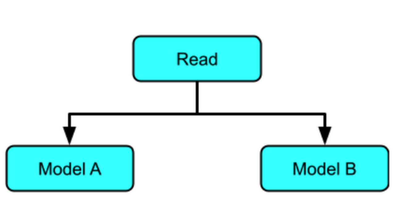
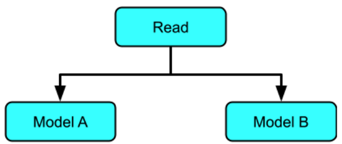
In part I of the series, the “join results from multiple models” pattern covered the various branching techniques in Apache Beam that make it possible to run data through multiple models.

Those techniques are applicable to RunInference API, which can easily be used by multiple branches within a pipeline, with the same or different models. This is similar in function to cascade ensembling, although here the data flows through multiple models in a single Apache Beam DAG.

Inference with multiple models in parallel

In this example, the same data is run through two different models: the one that we’ve been using to multiply by 5 and a new model, which will learn to multiply by 10.

Example of data being ran through 2 different models
"""
Create multiply by 10 table.

x is a range of values from 0 to 100.
y is a list of x * 10

value_to_predict includes a values outside of the training data
"""
x = numpy.arange( 0, 1000)
y = x * 10

# Create our labeled example file for 10 times table

example_ten_times_table = 'example_ten_times_table.tfrecord'

with tf.io.TFRecordWriter( example_ten_times_table ) as writer:
for i in zip(x, y):
example = ExampleProcessor().create_example_with_label(
feature=i[0], label=i[1])
writer.write(example.SerializeToString())

dataset = tf.data.TFRecordDataset(example_ten_times_table)
dataset = dataset.map(lambda e : tf.io.parse_example(e, RAW_DATA_TRAIN_SPEC))
dataset = dataset.map(lambda t : (t['x'], t['y']))
dataset = dataset.batch(100)
dataset = dataset.repeat()

model.fit(dataset, epochs=500, steps_per_epoch=10, verbose=0)

tf.keras.models.save_model(model,
save_model_dir_multiply_ten,
signatures=signature)

Now that we have two models, we apply them to our source data.

pipeline_options = PipelineOptions().from_dictionary(
{'temp_location':f'gs://{bucket}/tmp'})

pipeline = beam.Pipeline(options=pipeline_options)

with pipeline as p:
questions = p | beam.io.gcp.bigquery.ReadFromBigQuery(
table=f'{project}:maths.maths_problems_1')

multiply_five = ( questions
| "CreateMultiplyFiveTuple" >>
beam.Map(lambda x : (bytes('{}{}'.format(x['key'],' * 5'),'utf-8'),
ExampleProcessor().create_example(x['value'])))

| "Multiply Five" >> RunInference(
model_spec_pb2.InferenceSpecType(
saved_model_spec=model_spec_pb2.SavedModelSpec(
model_path=save_model_dir_multiply)))
)
multiply_ten = ( questions
| "CreateMultiplyTenTuple" >>
beam.Map(lambda x : (bytes('{}{}'.format(x['key'],'* 10'), 'utf-8'),
ExampleProcessor().create_example(x['value'])))
| "Multiply Ten" >> RunInference(
model_spec_pb2.InferenceSpecType(
saved_model_spec=model_spec_pb2.SavedModelSpec(
model_path=save_model_dir_multiply_ten)))
)
_ = ((multiply_five, multiply_ten) | beam.Flatten()
| beam.ParDo(PredictionWithKeyProcessor())
| beam.Map(print))
Output:

key is b'first_question * 5' input is [105.] output is 524.0875854492188
key is b'second_question * 5' input is [108.] output is 539.0093383789062
key is b'third_question * 5' input is [1000.] output is 4975.75830078125
key is b'fourth_question * 5' input is [1013.] output is 5040.41943359375
key is b'first_question* 10' input is [105.] output is 1054.333984375
key is b'second_question* 10' input is [108.] output is 1084.3131103515625
key is b'third_question* 10' input is [1000.] output is 9998.0908203125
key is b'fourth_question* 10' input is [1013.] output is 10128.0009765625

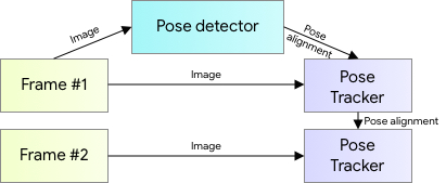
Inference with multiple models in sequence

In a sequential pattern, data is sent to one or more models in sequence, with the output from each model chaining to the next model.

sequential pattern sending data to one or more models in sequence, with the output from each model chaining to the next model.

Here are the steps:

  1. Read the data from BigQuery
  2. Map the data
  3. RunInference with multiply by 5 model
  4. Process the results
  5. RunInference with multiply by 10 model
  6. Process the results
pipeline_options = PipelineOptions().from_dictionary(
{'temp_location':f'gs://{bucket}/tmp'})

pipeline = beam.Pipeline(options=pipeline_options)

def process_interim_inference(element : Tuple[
bytes, prediction_log_pb2.PredictionLog
])-> Tuple[bytes, tf.train.Example]:

key = '{} original input is {}'.format(
element[0], str(tf.train.Example.FromString(
element[1].predict_log.request.inputs['examples'].string_val[0]
).features.feature['x'].float_list.value[0]))

value = ExampleProcessor().create_example(
element[1].predict_log.response.outputs['output_0'].float_val[0])

return (bytes(key,'utf-8'),value)

with pipeline as p:

questions = p | beam.io.gcp.bigquery.ReadFromBigQuery(
table=f'{project}:maths.maths_problems_1')

multiply = ( questions
| "CreateMultiplyTuple" >>
beam.Map(lambda x : (bytes(x['key'],'utf-8'),
ExampleProcessor().create_example(x['value'])))
| "MultiplyFive" >> RunInference(
model_spec_pb2.InferenceSpecType(
saved_model_spec=model_spec_pb2.SavedModelSpec(
model_path=save_model_dir_multiply)))

)

_ = ( multiply
| "Extract result " >>
beam.Map(lambda x : process_interim_inference(x))
| "MultiplyTen" >> RunInference(
model_spec_pb2.InferenceSpecType(
saved_model_spec=model_spec_pb2.SavedModelSpec(
model_path=save_model_dir_multiply_ten)))
| beam.ParDo(PredictionWithKeyProcessor())
| beam.Map(print)
)
Output: 

key is b"b'first_question' original input is 105.0" input is [524.9771118164062] output is 5249.7822265625
key is b"b'second_question' original input is 108.0" input is [539.9765014648438] output is 5399.7763671875
key is b"b'third_question' original input is 1000.0" input is [4999.7841796875] output is 49997.9453125
key is b"b'forth_question' original input is 1013.0" input is [5064.78125] output is 50647.91796875

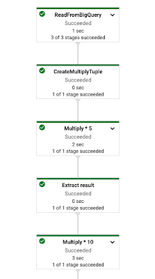
Running the pipeline on Dataflow

Until now the pipeline has been run locally, using the direct runner, which is implicitly used when running a pipeline with the default configuration. The same examples can be run using the production Dataflow runner by passing in configuration parameters including --runner. Details and an example can be found here.

Here is an example of the multimodel pipeline graph running on the Dataflow service:

example of the multimodel pipeline graph running on the Dataflow service

With the Dataflow runner you also get access to pipeline monitoring as well as metrics that have been output from the RunInference transform. The following table shows some of these metrics from a much larger list available from the library.

Table showing Dataflow runner metrics

Conclusion

In this blog, part II of our series, we explored the use of the tfx-bsl RunInference within some common scenarios, from standard inference, to post processing and the use of RunInference API in multiple locations in the pipeline.

To learn more, review the Dataflow and TFX documentation, you can also try out TFX with Google Cloud AI platform pipelines..

Acknowledgements

None of this would be possible without the hard work of many folks across both the Dataflow TFX and TF teams. From the TFX and TF team we would especially like to thank Konstantinos Katsiapis, Zohar Yahav, Vilobh Meshram, Jiayi Zhao, Zhitao Li, and Robert Crowe. From the Dataflow team I would like to thank Ahmet Altay for his support and input throughout.

Read More

Adaptive Framework for On-device Recommendation

Posted by Ellie Zhou, Tian Lin, Shuangfeng Li and Sushant Prakash

Introduction & Motivation

We are excited to announce an adaptive framework to build on-device recommendation ML solutions with your own data and advanced user modeling architecture.

After the previously open-sourced on-device recommendation solution, we received a lot of interest from the community on introducing on-device recommender AI. Motivated and inspired by the feedback, we considered various use cases, and created a framework that could generate TensorFlow Lite recommendation models accommodating different kinds of data, features, and architectures to improve the previous models.

Benefits of this framework:

  • Flexible: The adaptive framework allows users to create a model in a configurable way.
  • Better model representation: To improve the previous model, our new recommendation models can utilize multiple kinds of features than a single feature.

Personalized recommendations play an increasingly important role in digital life nowadays. With more and more user actions being moved to edge devices, supporting recommenders on-device becomes an important direction. Compared with conventional pure server-based recommenders, the on-device solution has unique advantages, such as protecting users’ privacy, providing fast reaction to on-device user actions, leveraging lightweight TensorFlow Lite inference, and bypassing network dependency. We welcome you to try out this framework and create recommendation experience in your applications.

In this article, we will

  • Introduce the improved model architecture and framework adaptivity.
  • Walk you through how to utilize the framework step-by-step.
  • Provide insights based on research done with a public dataset.

Please find more details on TensorFlow website.

Model

A recommendation model typically predicts users’ future activities, based on users’ previous activities. Our framework supports models using context information to do the prediction, which can be described in the following architecture:

recommendation code structure
Figure 1: An illustration of the configurable recommendation model. Each module is created according to the user-defined configuration.

At the context side, representations of all user activities are aggregated by the encoder to generate the context embedding. We support three different types of encoders: 1) bag-of-words (a.k.a. BOW), 2) 1-D convolution (a.k.a. CNN), and 3) LSTM. At the label side, the label item as positive and all other items in the vocabulary as negatives will be encoded to vectors as well. Context and label embeddings are combined with a dot product and fed to the loss of softmax cross entropy.

Inside the framework, we encapsulate tf.keras layers for ContextEncoder, LabelEncoder and DotProductSimilarity as key components in RecommendationModel.

To model each user activity, we could use the ID of the activity item (called ID-based), or multiple features of the item (called feature-based), or a combination of both. The feature-based model utilizing multiple features to collectively encode users’ behavior. With our framework, you could create either ID-based or feature-based models in a configurable way.

Similar to the last version, a TensorFlow Lite model will be exported after training which can directly provide top-K predictions among the recommendation candidates.

Step-by-step

To demonstrate the new adaptive framework, we trained a on-device movie recommendation model with MovieLens dataset using multiple features, and integrated it in the demo app. (Both the model and the app are for demonstration purposes only.) The MovieLens 1M dataset contains ratings from 6039 users across 3951 movies, with each user rating only a small subset of movies.

Let’s look at how to use the framework step-by-step in this notebook.

(a) Environment preparation

git clone https://github.com/tensorflow/examples
cd examples/lite/examples/recommendation/ml/
pip install -r requirements.txt

(b) Prepare training data

Please prepare your training data reference to the movielens example generation file. Would like to note that TensorFlow Lite input features are expected to be FixedLenFeature, please pad or truncate your features, and set up feature lengths in input configuration. Feel free to use the following command to process the example dataset.

python -m data.example_generation_movielens 
--data_dir=data/raw
--output_dir=data/examples
--min_timeline_length=3
--max_context_length=10
--max_context_movie_genre_length=32
--min_rating=2
--train_data_fraction=0.9
--build_vocabs=True

MovieLens data contains ratings.dat (columns: UserID, MovieID, Rating, Timestamp), and movies.dat (columns: MovieID, Title, Genres). The example generation script takes both files, only keep ratings higher than 2, form user movie interaction timelines, sample activities as labels and previous user activities as the context for prediction. Please find the generated tf.Example:

0 : {
features: {
feature: {
key : "context_movie_id"
value: { int64_list: { value: [ 1124, 2240, 3251, ..., 1268 ] } }
}
feature: {
key : "context_movie_rating"
value: { float_list: {value: [ 3.0, 3.0, 4.0, ..., 3.0 ] } }
}
feature: {
key : "context_movie_year"
value: { int64_list: { value: [ 1981, 1980, 1985, ..., 1990 ] } }
}
feature: {
key : "context_movie_id"
value: { int64_list: { value: [ 1124, 2240, 3251, ..., 1268 ] } }
}
feature: {
key : "context_movie_genre"
value: { bytes_list: { value: [ "Drama", "Drama", "Mystery", ..., "UNK" ] } }
}
feature: {
key : "label_movie_id"
value: { int64_list: { value: [ 3252 ] } }
}
}
}

(c) Create input config

Once data prepared, please set up input configuration, e.g. this is one example configuration for movielens movie recommendation model.

activity_feature_groups {
features {
feature_name: "context_movie_id"
feature_type: INT
vocab_size: 3953
embedding_dim: 8
feature_length: 10
}
features {
feature_name: "context_movie_rating"
feature_type: FLOAT
feature_length: 10
}
encoder_type: CNN
}
activity_feature_groups {
features {
feature_name: "context_movie_genre"
feature_type: STRING
vocab_name: "movie_genre_vocab.txt"
vocab_size: 19
embedding_dim: 4
feature_length: 32
}
encoder_type: CNN
}
label_feature {
feature_name: "label_movie_id"
feature_type: INT
vocab_size: 3953
embedding_dim: 8
feature_length: 1
}

(d) Train model

The model trainer will construct the recommendation model based on the input config, with a simple interface.

python -m model.recommendation_model_launcher -- 
--training_data_filepattern "data/examples/train_movielens_1m.tfrecord"
--testing_data_filepattern "data/examples/test_movielens_1m.tfrecord"
--model_dir "model/model_dir"
--vocab_dir "data/examples"
--input_config_file "configs/sample_input_config.pbtxt"
--batch_size 32
--learning_rate 0.01
--steps_per_epoch 2
--num_epochs 2
--num_eval_steps 2
--run_mode "train_and_eval"
--gradient_clip_norm 1.0
--num_predictions 10
--hidden_layer_dims "32,32"
--eval_top_k "1,5"
--conv_num_filter_ratios "2,4"
--conv_kernel_size 4
--lstm_num_units 16

Inside the recommendation model, core components are packaged up to keras layers (context_encoder.py, label_encoder.py and dotproduct_similarity.py), each of which could be utilized by itself. The following diagram illustrates the code structure:

An example of model architecture using context information to predict the next movie.
Figure 2: An example of model architecture using context information to predict the next movie. The inputs are the history of (a) movie IDs, (b) ratings and (c) genres, which is specified by the config mentioned above.

With the framework, you can directly execute the model training launcher with command:

python -m model.recommendation_model_launcher 
--input_config_file "configs/sample_input_config.pbtxt"
--vocab_dir "data/examples"
--run_mode "export"
--checkpoint_path "model/model_dir/ckpt-1000"
--num_predictions 10
--hidden_layer_dims "32,32"
--conv_num_filter_ratios "2,4"
--conv_kernel_size 4
--lstm_num_units 16

The inference code after exporting to TensorFlow Lite can be found in the notebook, and we refer readers to check out the details there.

Framework Adaptivity

Our framework provides a protobuf interface, through which feature groups, types and other information can be configured to build models accordingly. With the interface, you can configure:

  • Features

    The framework generically categorizes features into 3 types: integer, string, and float. Embedding spaces will be created for both integer and string features, hence, embedding dimension, vocabulary name and size need to be specified. Float feature values will be directly used. Besides, for on-device models, we suggest to use fixed length features which can be configured directly.

message Feature {
optional string feature_name = 1;

// Supported feature types: STRING, INT, FLOAT.
optional FeatureType feature_type = 2;

optional string vocab_name = 3;

optional int64 vocab_size = 4;

optional int64 embedding_dim = 5;

optional int64 feature_length = 6;
}
  • Feature groups

    One feature for one user activity may have multiple values. For instance, one movie can belong to multiple categories, each movie will have multiple genre feature values. To handle the different feature shapes, we introduced the “feature group” to combine features as a group . The features with the same length can be put in the same feature group to be encoded together. Inside input config, you can set up global feature groups and activity feature groups.

message FeatureGroup {
repeated Feature features = 1;

// Supported encoder types: BOW, CNN, LSTM.
optional EncoderType encoder_type = 2;
}
  • Input config

    You can use the input config interface to set up all the features and feature groups together.

message InputConfig {
repeated FeatureGroup global_feature_groups = 1;

repeated FeatureGroup activity_feature_groups = 2;

optional Feature label_feature = 3;
}

The input config is utilized by both input_pipeline.py and recommendation_model.py to process training data to tf.data.Dataset and construct the model accordingly. Inside ContexEncoder, FeatureGroupEncoders will be created for all feature groups, and used to compute feature group embeddings from input features. Concatenated feature group embeddings will be fed through top hidden layers to get the final context embedding. Worth noting that the final context embedding and label embedding dimensions should be equal.

Please check out the different model graphs produced with the different input configurations in the Appendix section.

Experiments and Analysis

We take this opportunity to analyze the performance of ID-based and feature-based models with various configurations, and provide some empirical results.

For the ID-based model, only movie_id is used as the input feature. And for the feature-based model, both movie_id and movie_genre features are used. Both types of models are experimented with 3 encoder types (BOW/CNN/LSTM) and 3 context history lengths (10/50/100).

Comparison between ID-based and Feature-based models.
Comparison between ID-based and Feature-based models. We compare them on BOW/CNN/LSTM encoders and context history lengths 10/50/100.

Since MovieLens dataset is an experimental dataset with ~4000 candidate movies and 19 movie genres, hence we scaled down embedding dimensions in the experiments to simulate the production scenario. For the above experiment result chart, ID embedding dimension is set to 8, and movie genre embedding dimension is set to 4. If we take the context10_cnn as an example, the feature-based model outperforms the ID-based model by 58.6%. Furthermore, the on average results show that feature-based models outperforms by 48.35%. Therefore, In this case, the feature-based model outperforms the ID-based model, because movie_genre feature introduces additional information to the model.

Besides, underlying features of candidate items mostly have a smaller vocabulary size, hence smaller embedding spaces as well. For instance,the movie genre vocabulary is much smaller than the movie ID vocabulary. In this case, utilizing underlying features could reduce the memory size of the model, which is more on-device friendly.

Acknowledgement

Special thanks to Cong Li, Josh Gordon, Khanh LeViet‎, Arun Venkatesan and Lawrence Chan for providing valuable suggestions to this work.

Read More

Reconstructing thousands of particles in one go at the CERN LHC with TensorFlow

A guest post by Jan Kieseler from CERN, EP/CMG

Introduction

At large colliders such as the CERN LHC (Large Hadron Collider) high energetic particle beams collide and thereby create massive and possibly yet unknown particles from the collision energy following the well known equation E=mc2. Most of these newly created particles are not stable and decay to more stable particles almost immediately. Detecting these decay products and measuring their properties precisely is the key to understanding what happened during the high energy collision, and will possibly shed light on big questions such as the origin of dark matter.

Detecting and measuring particles

For this purpose, the collision interaction points are surrounded by large detectors covering as much as possible in all possible directions and energies of the decay products. These detectors are further split into sub-detectors, each collecting complementary information. The innermost detector, closest to the interaction point, is the tracker consisting of multiple layers. Similar to a camera, each layer can detect the spatial position at which a charged particle passed through it, providing access to its trajectory. Combined with a strong magnetic field, this trajectory gives access to the particle charge and the particle momentum.

While the tracker is aimed at measuring the trajectories, only, while minimising any further interaction with and scattering of the particles, the next sub-detector layer is aimed at stopping them entirely. By stopping the particles completely, these calorimeters can extract the initial particle energy, and can also detect neutral particles. The only particles that pass through these calorimeters are muons, which are identified by additional muon chambers that constitute the outermost detector shell and use the same detection principles as the tracker.

Layout of the CMS detector, showing different particle species interacting with the sub-detectors (Image credit: CERN).

Combining the information from all these sub-detectors to reconstruct the final particles is a challenging task, not only because we want to achieve the best physics performance, but also in terms of computing resources and person-power available to develop and tune the reconstruction algorithms. In particular for the High-Luminosity LHC, the extension of the CERN LHC, aiming to collect unprecedented amounts of data, these algorithms need to perform well given a collision rate of 40MHz and up to 200 simultaneous interactions in each collision, which result in up to about a million signals from all sub-detectors.

Even with triggers, a fast, step-wise filtering of interesting events, in place, the total data collected to disk still comprises several petabytes, making efficient algorithms a must at all stages.

Classic reconstruction algorithms in high energy physics heavily rely on factorisation of individual steps and a lot of domain (physics) knowledge. While they perform reasonably well, the idealistic assumptions that are needed to develop these algorithms limit the performance, such that machine-learning approaches are often used to refine the classically reconstructed particles, and make their way into more and more reconstruction chains. The machine learning approaches benefit from a very precise simulation of all detector components and physics processes, valid over several orders of magnitude, such that large sets of labelled data can be produced very easily in a short amount of time. This led to a rise of neural network based identification and regression algorithms, and to the inclusion of TensorFlow as the standard inference engine in the software framework of the Compact Muon Solenoid (CMS) experiment.

Machine-learning reconstruction approaches also come with the advantage that by construction they have to be automatically optimizable and need a loss function to train that quantifies the final reconstruction target. In contrast, classic approaches are often optimised without the need to define such an inclusive quantitative metric, and parameters are tuned by hand, involving many experts, and taking a lot of person-power that could be spent on developing new algorithms instead of tuning existing ones. Therefore, moving to differentiable machine-learning algorithms such as deep neural networks in general can also help use the human resources more efficiently.

However, extending machine-learning based algorithms to the first step of reconstructing the particles from hits – instead of just refining already reconstructed particles – comes with two main challenges: the data structure and phrasing reconstruction as a minimisation problem.

The detector data is highly irregular, due to the inclusion of multiple sub-detectors, each with its own geometry. But even within a sub-detector, such as the tracker, the geometry is designed based on physics aspects with a fine resolution close to the interaction point and more coarse further away. Furthermore, the individual tracker layers are not densely packed, but have a considerable amount of space between them, and in each event only a small fraction of sensors are actually active, changing the number of inputs from event to event. Therefore, neural networks that require a regular grid, such as convolutional neural network architectures are – despite their good performance and highly optimised implementations – not applicable.

Graph neural networks can bridge this gap and, in principle, allow abstracting from the detector geometry. Recently, several graph neural network proposals from computer science have been studied in the context of refining already reconstructed particles in high energy physics. However, given the high input dimensionality of the data many of these proposals cannot be employed for reconstructing particles directly from hits, and custom solutions are needed. One example is GravNet that – by construction – reduces the resource requirements significantly while maintaining good physics performance by using sparse dynamic adjacency matrices and performing most operations without memory overhead.

This in particular becomes possible through TensorFlow which makes it easy to implement and load custom kernels into the graph and integrate custom analytic gradients for fused operations. Only the combination of these custom kernels and the network structure allows loading a full physics event into the GPU memory, training the network on it, and performing the inference.

GravNet layer architecture
GravNet layer architecture (from left to right): point features are projected into a feature space FLR, and a low dimensional coordinate space S; k nearest neighbours are determined in S; mean and maximum of distance weighted neighbour features are accumulated; accumulated features are combined with original features.

Since many of the reconstruction tasks, even the refinement of already reconstructed particles, rely on an unknown number of inputs, the recent addition and support of ragged data structures in TensorFlow in principle opens up a lot of new possibilities. While the integration is not sufficient to build full neural network architectures, yet, a future full support of ragged data structures would be a significant step forward for integrating TensorFlow even deeper into the reconstruction algorithms and would make some custom kernels obsolete.

The second challenge when reconstructing particles directly from hits using deep neural networks is to train the network to predict an unknown number of particles from an unknown number of inputs. There is a plethora of algorithms and training methods for detecting dense objects in dense data, such as images, but while the requirement of the dense data can be loosened in some cases, most of these algorithms still rely on the objects being dense or having a clear boundary, making it possible to exploit anchor boxes or central points of the object. Particles in the detector however, often overlap to a large degree, and their sparsity does not allow defining central points nor clear boundaries. A solution to this problem is Object Condensation, where object properties are condensed in at least one representative condensation point per object that can be chosen freely by the network through a high confidence score.

cluster points

To resolve ambiguities, the other points are clustered around the object they belong to using potential functions (illustrated above). However, these potentials scale with the confidence score in a tunable manner, such that the amount of segmentation the network should perform is adjustable up to the point where all points except the condensation points can be left free floating in case we are only interested in the final object properties.

Some parts of this algorithm are very similar to the method proposed in a previous paper, but the goal is entirely different. While the previous approach constitutes a very powerful segmentation algorithm moving pixels to cluster objects in an image towards a central point, the condensation points here directly carry object properties, and through the choice of the potential functions the clustering space can be completely detached from the input space. The latter has big implications for the applicability to the sparse detector data with overlapping particles, but also does not distinguish conceptually between “stuff” and “things”, providing a new perspective on one-shot panoptic segmentation.

But coming back to particle reconstruction, as shown in the corresponding paper, Object Condensation can outperform classic particle reconstruction algorithms even on simplified problems that are quite close to the idealistic assumptions of the classic algorithm. Therefore, it provides an alternative to classic reconstruction approaches directly from hits.

Based on this promising study, there is work ongoing to extend the approach to simulated events in the High Granularity Calorimeter, a planned new sub-detector of the CMS experiment at CERN, with about 2 million sensors, covering the particularly challenging forward region close to the incident beams, where most particles are produced. Compared to the published proof-of-concept, this realistic environment is much more challenging and requires the optimisation of the network structures and even more custom TensorFlow operations that can be found in the developing repository on github, using DeepJetCore as an interface to data formats commonly used in high-energy physics. Right now, there is a particular focus on implementing fast k-nearest-neighbour algorithms, a crucial building block for GravNet, that can handle the large input dimensionality, but also ragged implementations of other operations as well as implementations of the Object Condensation loss can be found there.

Conclusion

To conclude, the application of deep neural networks to reconstruction tasks is exhibiting a shift from refining classically reconstructed particles to reconstructing the particles and their properties directly, in an optimizable and highly parallelizable way to meet the person-power and computing challenges in the future. This development will give rise to more custom implementations, and will be using more of the bleeding edge features in TensorFlow and tf.keras such as ragged data structures, so that a closer contact between high-energy physics reconstruction developers and TensorFlow developers is foreseeable.

Acknowledgements

I would like to acknowledge the support of Thiru Palanisamy and Josh Gordon at Google for their help with the blog post collaboration and with providing active feedback.

Read More

How-to Write a Python Fuzzer for TensorFlow

Posted by Laura Pak

TensorFlow Python Fuzzer graphic

Fuzz testing is a process of testing APIs with generated data. Fuzzing ensures that code will not break on the negative path, generating randomized inputs that try to cover every branch of code. A popular choice is to pair fuzzers with sanitizers, which are tools that check for illegal conditions and thus flag the bugs triggered by the fuzzers’ inputs.

In this way, fuzzing can find:

  • Buffer overflows
  • Memory leaks
  • Deadlocks
  • Infinite recursion
  • Round-trip consistency failures
  • Uncaught exceptions
  • And more.

The best way to fuzz to have your fuzz tests running continuously. The more a test runs, the more inputs can be generated and tested against. In this article, you’ll learn how to add a Python fuzzer to TensorFlow.

The technical how-to

TensorFlow Python fuzzers run via OSS-Fuzz, the continuous fuzzing service for open source projects.

For Python fuzzers, OSS-Fuzz uses Atheris, a coverage-guided Python fuzzing engine. Atheris is based on the fuzzing engine libFuzzer, and it can be used with the dynamic memory error detector Address Sanitizer or the fast undefined behavior detector, Undefined Behavior Sanitizer. Atheris dependencies will be pre-installed on OSS-Fuzz base Docker images.

Here is a barebones example of a Python fuzzer for TF. The runtime will call TestCode with different random data.

import sys
import atheris_no_libfuzzer as atheris

def TestCode(data):
DoSomethingWith(data)

def main():
atheris.Setup(sys.argv, TestCode, enable_python_coverage=True)
atheris.Fuzz()

In the tensorflow repo, in the directory with the other fuzzers, add your own Python fuzzer like above. In TestCode, pick a TensorFlow API that you want to fuzz. In constant_fuzz.py, that API is tf.constant. That fuzzer simply passes data to the chosen API to see if it breaks. No need for code that catches the breakage; OSS-Fuzz will detect and report the bug.

Sometimes an API needs more structured data than just one input. TensorFlow has a Python class called FuzzingHelper that allows you to generate random int lists, a random bool, etc. See an example of its use in sparseCountSparseOutput_fuzz.py, a fuzzer that checks for uncaught exceptions in the API tf.raw_ops.SparseCountSparseOutput.

To build and run, your fuzzer needs a fuzzing target of type tf_py_fuzz_target, defined in tf_fuzzing.bzl. Here is an example fuzz target, with more examples here.

tf_py_fuzz_target(
name = "fuzz_target_name",
srcs = ["your_fuzzer.py"],
tags = ["notap"], # Important: include to run in OSS.
)

Testing your fuzzer with Docker

Make sure that your fuzzer builds in OSS-Fuzz with Docker.

First install Docker. In your terminal, run command docker image prune to remove any dangling images.

Clone oss-fuzz from Github. The project for a Python TF fuzzer, tensorflow-py, contains a build.sh file to be executed in the Docker container defined in the Dockerfile. Build.sh defines how to build binaries for fuzz targets in tensorflow-py. Specifically, it builds all the Python fuzzers found in $SRC/tensorflow/tensorflow, including your new fuzzer!

Inside oss-fuzz, run the following commands:

python infra/helper.py shell tensorflow
export FUZZING_LANGUAGE=python
compile

The command compile will run build.sh, which will attempt to build your new fuzzer.

The results

Once your fuzzer is up and running, you can search this dashboard for your fuzzer to see what vulnerabilities your fuzzer has uncovered.

Conclusion

Fuzzing is an exciting way to test software from the unhappy path. Whether you want to dabble in security or gain a deeper understanding of TensorFlow’s internals, we hope this post gives you a good place to start.

Read More

TensorFlow Quantum turns one year old

Posted by Michael Broughton, Alan Ho, Masoud Mohseni

Last year we announced TensorFlow Quantum (TFQ) at the 2020 TensorFlow developer summit and on the Google AI Blog. Bringing all of the tools and features that TensorFlow has to offer to the world of quantum computing has led to some great research success stories. In this post, we would like to look back on what’s happened in the last year involving TensorFlow Quantum and how far it’s come. We also discuss the future of quantum computing and machine learning in TensorFlow Quantum.

Since the release of TensorFlow Quantum, we’ve been happy to see increasing use of the library in the academic world as well as inside Alphabet, in particular the Quantum AI team at Google. There have been many research articles published in the last year that made use of TensorFlow Quantum in quantum machine learning or hybrid quantum-classical models, including discriminative models and generative models. With the cross pollination of ideas between the two fields, we are also seeing advanced learning algorithms from classical machine learning being reimagined such as quantum reinforcement learning, layerwise, and neural architecture search. We leverage the scalability and tooling of TensorFlow to run numerical experiments with large numbers of qubits and gates to more faithfully discover algorithms that will be practical in the future.

Here are a few papers published using TFQ if you’d like to check them out:

In our recent publication to quantify the computational advantage of quantum machine learning, experiments were conducted at PetaFLOP/s throughput scales, which is nothing new for classical machine learning, but represents a huge leap forward in the scale seen in quantum machine learning experiments before TensorFlow Quantum came along. We are very excited for the future that quantum computing and machine learning have together and we are happy to see TensorFlow Quantum having such a positive impact already.

The academic world isn’t the only place machine learning and quantum computing have been able to come together. Over the past year members of the TensorFlow Quantum team helped out in supporting the artistic works of Refik Anadol Studios’ “Quantum memories” piece. This combines the random circuit sample data from the 2019 beyond classical experiment and adoptions of StyleGAN to create some truly magnificent works of art

Quantum memories installation at the NGV (image used with permission).

Next steps

We will soon be releasing TensorFlow Quantum 0.5.0, with more support for distributed workloads as well as lots of new quantum centric features and some small performance boosts. Looking forward, we hope that these features will enable our users to continue to push the boundaries of complexity and scale in quantum computing and machine learning and eventually help lead to groundbreaking quantum computing experiments (not just simulations). Our ultimate goal when we released TensorFlow Quantum was to have it aid in the search for quantum advantage in the field of machine learning. In time, it is our hope to see the world reach that goal, with the help of the continued hard work and dedication of the QML research community. Quantum machine learning is still a very young field and there’s still a long way to go before this happens, but over the past year we’ve seen the community make amazing strides in many different areas and we can’t wait to see what you will accomplish in the years to come.

Read More

A Tour of SavedModel Signatures

Posted by Daniel Ellis, TensorFlow Engineer

Note: This blog post is aimed at TensorFlow developers who want to learn the details of how graphs and models are stored. If you are new to TensorFlow, you should check out the TensorFlow Basics guides before reading this article.

TensorFlow can run models without the original Python objects, as demonstrated by TensorFlow Serving and TensorFlow Lite, or when you download a trained model from TensorFlow Hub.

Models and layers can be loaded from this representation without actually making an instance of the Python class that created it. This is desired in situations where you do not have (or want) a Python interpreter, such as serving at scale or on an edge device, or in situations where the original Python code is not available.

Saved models are represented by two separate, but equally important, parts: the graph, which describes the fixed computation described in code, and the weights, which are the dynamic parameters you trained during training. If you aren’t already familiar with this and @tf.function, you should check out the Introduction to graphs and functions guide as well as the section on saving in the modules, layers, and models guide.

From a code standpoint, functions decorated with @tf.function create a Python callable; in the documentation we refer to these as polymorphic functions, as they are Python callables that can take a variety argument signatures. Each time you call a @tf.function with a new argument signature, TensorFlow traces out a new graph just for that set of arguments. This new graph is then added as a “concrete function” to the callable. Thus, a saved model can be one or more subgraphs, each with a different signature.

A SavedModel is what you get when you call tf.saved_model.save(). Saved models are stored as a directory on disk. The file, saved_model.pb,within that directory, is a protocol buffer describing the functional tf.Graph.

In this blog post, we’ll take a look inside this protobuf and see how function signature serialization and deserialization works under the hood. After reading this, you’ll have a greater appreciation for what functions and signatures before, which can help you load, modify, or optimize saved models.

Background

There are a total of five places inputs to functions are defined in the saved model protobuf. It can be tough to understand and remember what each of these does. This post intends to inventory each of these definitions and what they’re used for. It also goes through a basic example illustrating what a simple model looks like after serialization.

The actual APIs you use will always be carefully versioned (as they have been since 2016), and the models themselves will conform to the version compatibility guide. However, the material in this document lays out a snapshot of the existing state of things. Any links to code will include point-in-time revisions so as not to drift out of date. As with all non-documented implementation details, these details are subject to change in the future.

We’ll occasionally use the term “signatures” to talk about the general concept of describing function inputs (e.g. in the title of this document). In this sense, we will be referring not just to TensorFlow’s specific concept of signatures, but all of the ways TensorFlow defines and validates inputs to functions. Context should make the meaning clear.

What This Is Not About

This document is not intended to describe how signatures or functions work from a user perspective. It is intended for TensorFlow developers working on the internals of TensorFlow. Likewise, this document does not make a statement of the way things “should” be. It aims to simply document the way things are.

Overview of Signature Definitions

There are five protos that store definitions of function inputs in one manner or another. Their names and code locations, as well as their paths within the saved model proto, are as follows:

Proto messages, and their location in SavedModel

FunctionDef

Of the five definitions discussed in this document, FunctionsDefs are the most core to execution. When loading a saved model, these function definitions are registered in the function library of the runtime and used to create ConcreteFunctions. These functions can then be executed via PartitionedCall or TFE_Py_Execute.

This is where the actual nodes describing execution are defined, as well as what the inputs and outputs to the function are.

SignatureDef

SignatureDefs are generated from signatures passed into @tf.function. We do not save the signature’s TensorSpecs directly, however. Instead, when saving, we call the underlying function using the TensorSpecs in order to generate a concrete function. From there, we inspect the generated concrete function to get the inputs and outputs, storing them on the SignatureDef.

On the loading side,SignatureDefs are essentially ignored. They are primarily used in v1 or C++, where the developer loading the model can inspect the returned SignatureDef protos directly. This allows them to use their desired signature name to lookup the placeholder and output names needed for execution.

These input and output names can then be passed into feeds and fetches when calling Session.run in TensorFlow V1 code.

SavedFunction

SavedFunction is one of the many types of SavedObjects in the nodes list of the ObjectGraphDef. SavedFunctions are restored into a RestoredFunctions at load time. Like all nodes in this list, they are then attached to the returned model via the hierarchy defined by the children ObjectReference field.

SavedFunction’s main purpose is polymorphism. SavedFunctions support polymorphism by specifying a number of concrete function names defined in the function library above (via FunctionDef). At call time, we iterate through the concrete function names to find the first whose signature matches. If we find a match, we call it; if not, we throw an exception.

There is one more bit of complexity. When a RestoredFunction is called with a particular set of arguments, a new concrete function is created whose sole purpose is to call the matching concrete function. This is done using restored_function_body under the hood and is where the logic lives to find the appropriate concrete function.

This is invisible in the SavedModel proto, but these extra concrete functions are registered at call time in the runtime’s function library just as the other function library functions are.

The second purpose of SavedFunction is to update the FunctionSpec of all associated ConcreteFunctions using the FunctionSpec stored on the SavedFunction. This function spec is used at call time to

  1. validate passed in structured arguments, and
  2. convert structured arguments into flat ones needed for calling the underlying concrete function.

SavedBareConcreteFunction

Similar to SavedFunctions, SavedBareConcreteFunctions are used to update a

specific concrete function’s arguments and function spec. This is done here. Unlike SavedFunctions, they only reference a single specific concrete function.

In practice, SavedBareConcreteFunctions are commonly attached to and accessed via the signatures map (i.e. the signatures attribute on the loaded object). The underlying concrete functions they modify, in this case, are signature_wrapper functions. This wrapping is done to format the output in the way v1 expects (i.e. a dictionary of tensors). Similar to restored_function_body concrete functions, and other than restructuring the output, these concrete functions do nothing but call their associated concrete functions.

SavedConcreteFunction

SavedConcreteFunction objects are not SavedObjectGraph nodes. They are stored in a map directly on the SavedObjectGraph. These objects reference a specific, already-registered concrete function — the key in the map is that concrete function’s registered name.

These objects serve two purposes. The first is handling function “captures” via

the bound_inputs field. Captured variables are those a function reads or modifies that were not explicitly passed in when calling into the function. Since functions in the function library do not have a concept of captured variables, any variables used by the function must be passed in as an argument. bound_inputs stores a list of node IDs that should be passed in to the underlying ConcreteFunction when called. We set this up here.

The second purpose, and similar to SavedFunction and SavedBareConcreteFunction, is modifying the existing concrete function’s FuncGraph structured inputs and outputs. This also is used for argument validation. The setup for this is done here.

Example Walkthrough

A simple example may help illustrate all of this with more clarity. Let’s make a basic model and take a look at the subsequent generated proto to get a better feel for what’s going on.

Basic Model

class ExampleModel(tf.Module):

@tf.function(input_signature=[tf.TensorSpec(shape=(), dtype=tf.float32)])
def capture_fn(self, x):
if not hasattr(self, 'weight'):
self.weight = tf.Variable(5.0, name='weight')
self.weight.assign_add(x * self.weight)
return self.weight

@tf.function
def polymorphic_fn(self, x):
return tf.constant(3.0) * x

model = ExampleModel()
model.polymorphic_fn(tf.constant(4.0))
model.polymorphic_fn(tf.constant([1.0, 2.0, 3.0]))
tf.saved_model.save(
model, "/tmp/example-model", signatures={'capture_fn': model.capture_fn})

This model contains the basis for most of the complexity we’ll need to fully explore the intricacies of saving and signatures. This will allow us to look at functions with and without signatures, with and without captures, and with and without polymorphism.

Function with Captures

Let’s start by looking at our function with captures, capture_fn. We can see we have a concrete function defined in the function library, as expected:

Image of concrete function defined in the function library
A FunctionDef located in FunctionDefLibrary of MetaGraphDef.graph_def

Note the expected float input, "x", as well as the additional captured argument, "mul_readvariableop_resource". Since this function has a capture, we should see a variable being referenced in the bound_inputs field of one of our SavedConcreteFunctions:

SavedConcreteFunctions
A SavedConcreteFunction located in the concrete_functions map of the ObjectGraphDef

Indeed, we can see bound_inputs refers to node 1, which is a SavedVariable with the name and dtype we expect:

A `SavedVariable` located in `ObjectGraphDef.nodes`
A SavedVariable located in ObjectGraphDef.nodes

Note that we also are storing on canonicalized_input_signature additional data that will be used to modify the concrete function. The key of this object, "__inference_capture_fn_59", is the same name as the concrete function registered in our function library.

Since we’ve specified a signature, we should also see a SavedBareConcreteFunction:

SavedBareConcreteFunction
A SavedBareConcreteFunction located in ObjectGraphDef.nodes

As discussed above, we use the function spec and argument information to modify the underlying concrete function. But what’s up with the "__inference_signature_wrapper_68" name? And how does this fit in with the rest of the code?

First, note that this is the fifth (5) node in the node list. This will come up again shortly.

Let’s start by looking at the nodes list. If we start at the first node in the nodes list, we’ll see a "signatures" node attached as a child:

SavedUserObject
A SavedUserObject located in ObjectGraphDef.nodes

If we look at node 2, we’ll see this node is a signature map that references one final node: node 5, our BareConcreteSavedFunction.

Node5
A SavedUserObject located in ObjectGraphDef.nodes

Thus, when we access this function via model.signatures["capture_fn"], we will actually be calling into this intermediate signature wrapper function first.

And what does that function, "__inference_signature_wrapper_68", look like?

FunctionDef
A FunctionDef located in FunctionDefLibrary of MetaGraphDef.graph_def

It takes the arguments we expect, and makes a call out to… "__inference_capture_fn_59", our original function! Just as we expect.

But wait… what happens if we don’t access our function via model.signatures["capture_fn"]? After all, we should be able to call it directly via model.capture_fn.

Notice above, we had a child on the top level object named "capture_fn" with a node_id of 3. If we look at node 3, we’ll see a SavedFunction object that references our original concrete function with no signature wrapper intermediary:

Node 3
A SavedFunction located in ObjectGraphDef.nodes

Again, the function spec is used to modify the function spec of our concrete function, "__inference_capture_fn_59". Notice also that concrete_functions here is a list. We only have one item right now, but this will come up again when we take a look at our polymorphic function example.

Now, we’ve fully mapped essentially everything needed for execution of this function, but we have one last thing to look at: SignatureDef. We’ve defined a signature, so we expect a SignatureDef to be defined:

SignatureDef
A SignatureDef located in the MetaObjectGraph.signature_def map

This is very important for loading in v1 and C++ for serving. Note those funky names: "capture_fn_x:0" and "StatefulPartitionedCall:0". To call this function in v1, we need a way to map our nice argument names to the actual graph placeholder names for passing in as feeds and fetches (and doing validation, if we wish). Looking at this SignatureDef allows us to do just that.

Polymorphic Functions

We’re not quite done yet. Let’s take a look at our polymorphic function. We won’t repeat everything, since a lot of it is the same. We won’t have any signature wrapper functions or signature defs, since we skipped the signature on this one. Let’s look at what’s different.

A Polymorphic FunctionDef
A FunctionDef located in FunctionDefLibrary of MetaGraphDef.graph_def

For one, we now have two concrete functions registered in the function library, each with slightly different input shapes.

We also have two SavedConcreteFunction modifiers:

Two SavedConcreteFunctions
Two SavedConcreteFunctions located in the concrete_functions map of the ObjectGraphDef

And finally, we can see our SavedFunction references two underlying concrete functions instead of one:

SavedFunction
A SavedFunction located in ObjectGraphDef.nodes

The function spec here will be attached to both of these concrete functions at load time. When we call our SavedFunction, it will use the arguments we pass in to find the correct concrete function and execute it.

Next Steps

You should now be an expert on how functions and their signatures are saved at a code level. Remember, what’s described in this blog post is how the code works right now. For updated code and examples in the future, see the official documentation on tensorflow.org.

Speaking of documentation, if you want a fast introduction to the basic APIs for saved models, you should introductory articles on how the APIs for functions and modules are traced and saved. For experts, don’t miss this detailed guide on SavedModel itself, as well as a complete discussion of autograph.

And finally, if you do any exciting or useful protobuf surgery, share with us on Twitter. Thanks for reading this far!

Read More

Transfer Learning for Audio Data with YAMNet

Posted by Luiz GUStavo Martins, Developer Advocate

Transfer learning is a popular machine learning technique, in which you train a new model by reusing information learned by a previous model. Most common applications of transfer learning are for the vision domain, to train accurate image classifiers, or object detectors, using a small amount of data — or for text, where pre-trained text embeddings or language models like BERT are used to improve on natural language understanding tasks like sentiment analysis or question answering. In this article, you’ll learn how to use transfer learning for a new and important type of data: audio, to build a sound classifier.

There are many important use cases of audio classification, including to protect wildlife, to detect whales and even to fight against illegal deforestation.

With YAMNet, you can create a customized audio classifier in a few easy steps:

  • Prepare and use a public audio dataset
  • Extract the embeddings from the audio files using YAMNet
  • Create a simple two layer classifier and train it.
  • Save and test the final model

You can follow the code here in this tutorial.

The YAMNet model

YAMNet (“Yet another Audio Mobilenet Network”) is a pretrained model that predicts 521 audio events based on the AudioSet corpus.

This model is available on TensorFlow Hub including the TFLite and TF.js versions, for running the model on mobile and the web. The code can be found on their repository.

The model has 3 outputs:

  • Class scores that you’d use for inference
  • Embeddings, which are the important part for transfer learning
  • Log Mel Spectrograms to provide a visualization of the input signal

The model takes a waveform represented as 16 kHz samples in the range [-1.0, 1.0], frames it in windows of 0.96 seconds and hop of 0.48 seconds, and then runs the core of the model to extract the embeddings on a batch of these frames.

The 0.96 seconds windows hopping over a waveform

As an example, trying the model with this audio file [link] will give you these results:

The first graph is the waveform. The second graph is the log-mel spectrogram. The third graph shows the class probability predictions per frame of audio, where darker is more likely.

The ESC-50 dataset

To do transfer learning with the model, you’ll use the Dataset for Environmental Sound Classification, or ESC-50 for short. This is a collection of 2000 environmental audio recordings from 50 classes. Each recording is 5 seconds long and they came originally from the Freesound project.

The ESC-50 has the classes Dog and Cat that you’ll need.

The dataset has two important components: the audio files and a metadata csv file with the metadata about every audio file.

The columns in the metadata csv file contains information that will be used to train the model:

  • Filename gives the name of the .wav audio file
  • Category is the human-readable class name for the numeric target id
  • Target is the unique numeric id of the category
  • Fold ensures that clips originating from the same initial source are always contained in the same group. This is important to avoid cross-contamination when splitting the data into train, validation and test sets and for cross-validation.

For more detailed information you can read the original ESC paper.

Working with the dataset

To load the dataset, you’ll start from the metadata file and load it using the Pandas method read_csv.

With the loaded dataframe, the next steps are to filter by the classes that will be used, in this case: Dogs and Cats.

Next step would be to load the audio files to start the process but if there are too many audio files, just loading all of them to memory can be prohibitive and lead to out of memory issues. The best solution is to lazily load the audio files when needed. TensorFlow can help do this easily with tf.data.Dataset and the map method.

Let’s create the Dataset from the the previous created pandas dataframe and apply the load_wav method to all the files:

filenames = filtered_pd['filename']
targets = filtered_pd['target']
folds = filtered_pd['fold']

main_ds = tf.data.Dataset.from_tensor_slices((filenames, targets, folds))
main_ds = main_ds.map(load_wav_for_map)

Here, no audio file was loaded to memory yet since the mapping wasn’t evaluated. For example, if you request a size of the dataset for example (len(list(train_ds.as_numpy_iterator()))

), that would make the map function to be evaluated and load all the files.

The same technique will be used to extract all the features (embeddings) from each audio file.

Extracting the audio embeddings

Here you are going to load the YAMNet model from TensorFlow Hub. All you need is the model’s handle, and call the load method from the tensorflow_hub library.

yamnet_model_handle = 'https://tfhub.dev/google/yamnet/1'
yamnet_model = hub.load(yamnet_model_handle)

This will load the model to memory ready to be used.

For each audio file, you’ll extract the embeddings using the YAMNet model. For each audio file, YAMNet is executed. The embeddings output is paired with the same label and folder from the audio file.

def extract_embedding(wav_data, label, fold):
''' run YAMNet to extract embedding from the wav data '''
scores, embeddings, spectrogram = yamnet_model(wav_data)
num_embeddings = tf.shape(embeddings)[0]
return (embeddings,
tf.repeat(label, num_embeddings),
tf.repeat(fold, num_embeddings))

main_ds = main_ds.map(extract_embedding).unbatch()

These embeddings will be the input for the classification model. From the model’s documentation, you can read that for a given audio file, it will frame the waveform into sliding windows of length 0.96 seconds and hop 0.48 seconds, and then run the core of the model. So, in summary, for each 0.48 seconds, the model will output one embedding array with 1024 float values. This part is also done using map(), so again, lazy evaluation and that’s why it executes so fast.

The final dataset contains the three used columns: embedding, label and fold.

The last dataset operation is to split into train, validation and test datasets. To do so the filter() method and use the fold field (an integer between 1 and 5) as criteria.

cached_ds = main_ds.cache()
train_ds = cached_ds.filter(lambda embedding, label, fold: fold < 4)
val_ds = cached_ds.filter(lambda embedding, label, fold: fold == 4)
test_ds = cached_ds.filter(lambda embedding, label, fold: fold == 5)

Training the Classifier

With the YAMNet embedding vectors and the label, the next step is to train a classifier that learns what’s a dog’s sound and what is a cat’s sound.

The classifier model is very simple with just two dense layers, but as you’ll see this is enough for the amount of data used.

my_model = tf.keras.Sequential([
tf.keras.layers.Input(shape=(1024), dtype=tf.float32, name='input_embedding'),
tf.keras.layers.Dense(512, activation='relu'),
tf.keras.layers.Dense(len(my_classes))
])

Saving the final model

The model that was trained works and has good accuracy but the input it expects is not an audio waveform but an embedding array. To address this problem, the final model will combine YAMNet as the input layer and the model just trained. This way, the final model will accept a waveform and output the class:

input_segment = tf.keras.layers.Input(shape=(), dtype=tf.float32,
name='audio')
embedding_extraction_layer = hub.KerasLayer('https://tfhub.dev/google/yamnet/1', trainable=False)
scores, embeddings, spectrogram = embedding_extraction_layer(input_segment)
serving_outputs = my_model(embeddings_output)
serving_outputs = ReduceMeanLayer(axis=0, name='classifier')(serving_outputs)
serving_model = tf.keras.Model(input_segment, serving_outputs)
serving_model.save(saved_model_path, include_optimizer=False)

To try the reloaded model, you can use the same way it was used earlier in the colab:

reloaded_model = tf.saved_model.load(saved_model_path)
reloaded_results = reloaded_model(testing_wav_data)
cat_or_dog = my_classes[tf.argmax(reloaded_results)]

This model can also be used with TensorFlow Serving with the ‘serving_default’

serving_results =  reloaded_model.signatures['serving_default'](testing_wav_data)
cat_or_dog = my_classes[tf.argmax(serving_results['classifier'])]

In this post, you learned how to use the YAMNet model for transfer learning to recognize audio of dogs and cats from the ESC-50 dataset.

Check out the YAMNet model on tfhub.dev and the tutorial on tensorflow.org. You can apply this technique to your own dataset, or to other classes in the ESC-50 dataset.

We would love to know what you can build with this! Share your project with us on social media by using the hashtag #TFHub.

Acknowledgements

We’d like to thank a number of colleagues for their contribution to this work: Dan Ellis, Manoj Plakal and Eduardo Fonseca for an amazing YAMNet model and support with the colab and multiple reviews.

Mark Daoust and Elizabeth Kemp have greatly improved the presentation of the material in this post and the associated tutorial.

Read More

Introducing TensorFlow Videos for a Global Audience: Vietnamese

Posted by TensorFlow Team

When the TensorFlow YouTube channel launched in 2018, we had a vision to inform and inspire developers around the world about what was possible with Machine Learning. With series like Coding TensorFlow showing how you can use it, and Made with TensorFlow showing inspirational stories about what people have done with TensorFlow and much more, the channel has grown greatly. But we learned an important lesson: it’s a global phenomenon, and to reach the world effectively, we should provide some of our content in multiple languages with native speakers presenting. Check out the popular Zero to Hero series in Vietnamese!

Nhập môn Học máy với TensorFlow

Dường như mỗi khi bạn lướt web, đọc sách, báo thì thông tin về công nghệ học máy (machine learning) và trí tuệ nhân tạo (AI) luôn đập vào mắt bạn. Trong số đó cũng có không ít những thông tin và quảng cáo thổi phồng về AI. Bởi vậy, từ góc nhìn của developer, chúng tôi trong nhóm TensorFlow quyết định sản xuất một chuỗi video gồm 4 phần về bản chất thực sự của công nghệ học máy, dựa trên bài thuyết trình nổi tiếng của Laurence Moroney tại Google IO 2019 với tựa đề Machine Learning: Zero to Hero (tạm dịch là Công nghệ Học máy: Trở thành chuyên gia từ con số 0 với TensorFlow).

Trong video 1, chúng tôi sẽ giới thiệu về một hình thức lập trình mới là học máy. Trong đó, thay vì lập trình các chỉ thị cho máy tính bằng ngôn ngữ lập trình như Java hoặc C++, thì trong học máy bạn sẽ tạo một chương trình được huấn luyện dựa trên dữ liệu và máy tính sẽ tự suy ra các logic từ dữ liệu này. Vậy công nghệ học máy thực sự là như thế nào? Chúng ta sẽ cùng tìm hiểu về một ví dụ “Hello World” về tạo mô hình học máy, giới thiệu các ý tưởng mà chúng ta sau đó sẽ áp dụng cho một vấn đề thú vị hơn: thị giác máy tính.

Trong video 2, bạn sẽ tìm hiểu về thị giác máy tính dựa trên học máy. Chúng ta sẽ huấn luyện cho máy tính nhìn thấy và nhận diện các đồ vật khác nhau.

Trong video 3, chúng ta sẽ học về các mạng nơ ron tích chập và lý do chúng đóng vai trò quan trọng trong các ứng dụng thị giác máy tính. Tích chập là bộ lọc xử lý hình ảnh và trích xuất các đặc điểm đặc trưng của ảnh. Bạn sẽ tìm hiểu về cách hoạt động của các mạng nơ ron tích chập qua việc xử lý và trích xuất đặc điểm của một tập các hình ảnh thực tế.

Trong video 4, bạn sẽ học về cách xây dựng mô hình phân loại hình ảnh để chơi trò oẳn tù tì. Trong phần 1, chúng ta đã đề cập đến trò chơi oẳn tù tì và việc lập trình để máy tính nhận biết hình ảnh bàn tay ra đấm, lá, kéo khó như thế nào. Tuy nhiên, sau đó chúng ta cũng đã tìm hiểu nhiều về công nghệ học máy, cách xây dựng mạng nơ ron để phát hiện các quy luật từ dữ liệu điểm ảnh, và phương pháp sử dụng mạng tích chập để phát hiện các đặc trưng trong bức ảnh. Trong phần này, chúng ta đã áp dụng những kiến thức đã học từ 3 phần trước để xây dựng mạng nơ ron để máy tính chơi oẳn tù tì.

Hy vọng loạt video này sẽ giúp bạn làm quen với học máy. Nếu có góp ý gì, các bạn hãy viết vào phần comment trong video trên YouTube. Và đừng quên subscribe kênh YouTube của TensorFlow thể xem các video khác về học máy nữa nhé!

Read More

Variational Inference with Joint Distributions in TensorFlow Probability

Posted by Emily Fertig, Joshua V. Dillon, Wynn Vonnegut, Dave Moore, and the TensorFlow Probability team

In this post, we introduce new tools for variational inference with joint distributions in TensorFlow Probability, and show how to use them to estimate Bayesian credible intervals for weights in a regression model.

Overview

Variational Inference (VI) casts approximate Bayesian inference as an optimization problem and seeks a ‘surrogate’ posterior distribution that minimizes the KL divergence with the true posterior. Gradient-based VI is often faster than MCMC methods, composes naturally with optimization of model parameters, and provides a lower bound on model evidence that can be used directly for model comparison, convergence diagnosis, and composable inference.

TensorFlow Probability (TFP) offers tools for fast, flexible, and scalable VI that fit naturally into the TFP stack. These tools enable the construction of surrogate posteriors with covariance structures induced by linear transformations or normalizing flows.

VI can be used to estimate Bayesian credible intervals for parameters of a regression model to estimate the effects of various treatments or observed features on an outcome of interest. Credible intervals bound the values of an unobserved parameter with a certain probability, according to the posterior distribution of the parameter conditioned on observed data and given an assumption on the parameter’s prior distribution.

In this post, we demonstrate how to use VI to obtain credible intervals for parameters of a Bayesian linear regression model for radon levels measured in homes (using Gelman et al.’s (2007) Radon dataset; see similar examples in Stan). We demonstrate how TFP JointDistributions combine with bijectors to build and fit two types of expressive surrogate posteriors:

  • a standard Normal distribution transformed by a block matrix. The matrix may reflect independence among some components of the posterior and dependence among others, relaxing the assumption of a mean-field or full-covariance posterior.
  • a more complex, higher-capacity inverse autoregressive flow.

The surrogate posteriors are trained and compared with results from a mean-field surrogate posterior baseline. These plots show credible intervals for four model parameters obtained with the three VI surrogate posteriors, as you’ll learn about below, as well as Hamiltonian Monte Carlo (HMC) for comparison.

credible intervals for four model parameters obtained with the three VI surrogate posteriors

You can follow along and see all the details in this Google Colab.

Example: Bayesian hierarchical linear regression on Radon measurements

Radon is a radioactive gas that enters homes through contact points with the ground. It is a carcinogen that is the primary cause of lung cancer in non-smokers. Radon levels vary greatly from household to household.

The EPA did a study of radon levels in 80,000 houses. Two important predictors are:

  • Floor on which the measurement was taken (radon higher in basements)
  • County uranium level (positive correlation with radon levels)

Predicting radon levels in houses grouped by county is a classic problem in Bayesian hierarchical modeling, introduced by Gelman and Hill (2006). We are interested in credible intervals for the effect of location (county) on the radon level of houses in Minnesota. In order to isolate this effect, the effects of floor and uranium level are also included in the model. Additionally, we will incorporate a contextual effect corresponding to the mean floor on which the measurement was taken, by county, so that if there is variation among counties of the floor on which the measurements were taken, this is not attributed to the county effect.

The regression model is specified as follows:

Regression model

in which i indexes the observations and countyi is the county in which the ith observation was taken.

We use a county-level random effect to capture geographical variation. The parameters uranium_weight and county_floor_weight are modeled probabilistically, and floor_weight and the constant bias are deterministic. These modeling choices are largely arbitrary, and are made for the purpose of demonstrating VI on a probabilistic model of reasonable complexity. For a more thorough discussion of multilevel modeling with fixed and random effects in TFP, using the radon dataset, see Multilevel Modeling Primer and Fitting Generalized Linear Mixed-effects Models Using Variational Inference.

The full code for this example is available on Github.

Variables are defined for the deterministic parameters and the Normal distribution scale parameters, with the latter constrained to be positive.

import tensorflow as tf
import tensorflow_probability as tfp
tfd = tfp.distributions
tfb = tfp.bijectors

floor_weight = tf.Variable(0.)
bias = tf.Variable(0.)
log_radon_scale = tfp.util.TransformedVariable(1., tfb.Exp())
county_effect_scale = tfp.util.TransformedVariable(1., tfb.Exp())

We specify the probabilistic graphical model for the regression as a TFP JointDistribution.

@tfd.JointDistributionCoroutineAutoBatched
def model():
uranium_weight = yield tfd.Normal(0., scale=1., name='uranium_weight')
county_floor_weight = yield tfd.Normal(
0., scale=1., name='county_floor_weight')
county_effect = yield tfd.Sample(
tfd.Normal(0., scale=county_effect_scale),
sample_shape=[num_counties], name='county_effect')
yield tfd.Normal(
loc=(log_uranium * uranium_weight
+ floor_of_house * floor_weight
+ floor_by_county * county_floor_weight
+ tf.gather(county_effect, county, axis=-1)
+ bias),
scale=log_radon_scale[..., tf.newaxis],
name='log_radon')

We pin log_radon to the observed radon data to model the unnormalized posterior.

target_model = model.experimental_pin(log_radon=log_radon)

Quick summary of Bayesian Variational Inference

Suppose we have the following generative process, where 𝜃 represents random parameters (uranium_weight, county_floor_weight, and county_effect in the regression model) and ω represents deterministic parameters (floor_weight, log_radon_scale, county_effect_scale, and bias). The x𝑖 are features (log_uranium, floor_of_house, and floor_by_county) and the 𝑦𝑖 are target values (log_radon) for 𝑖 = 1…n observed data points:

equation

VI is then characterized by:

equation

(Technically we’re assuming q is absolutely continuous with respect to r. See also, Jensen’s inequality.)

Since the bound holds for all q, it is obviously tightest for:

equation

Regarding terminology, we call

  • q* the “surrogate posterior,” and,
  • Q the “surrogate family.”

ω* represents the maximum-likelihood values of the deterministic parameters on the VI loss. See this survey for more information on variational inference.

Expressive surrogate posteriors

Next we estimate the posterior distributions of the parameters using VI with two different types of surrogate posteriors:

  • A constrained multivariate Normal distribution, with covariance structure induced by a blockwise matrix transformation.
  • A multivariate standard Normal distribution transformed by an Inverse Autoregressive Flow, which is then split and restructured to match the support of the posterior.

Multivariate Normal surrogate posterior

To build this surrogate posterior, a trainable linear operator is used to induce correlation among the components of the posterior.

We begin by constructing a base distribution with vector-valued standard Normal components, with sizes equal to the sizes of the corresponding prior components. The components are vector-valued so they can be transformed by the linear operator.

flat_event_size = tf.nest.map_structure(
tf.reduce_prod,
tf.nest.flatten(target_model.event_shape_tensor()))
base_standard_dist = tfd.JointDistributionSequential(
[tfd.Sample(tfd.Normal(loc=0., scale=1.), s)
for s in flat_event_size])

To this distribution, we apply a trainable blockwise lower-triangular linear operator to induce correlation in the posterior. Within the linear operator, a trainable full-matrix block represents full covariance between two components of the posterior, while a block of zeros (or None) expresses independence. Blocks on the diagonal are either lower-triangular or diagonal matrices, so that the entire block structure represents a lower-triangular matrix.

Applying this bijector to the base distribution results in a multivariate Normal distribution with mean 0 and (Cholesky-factored) covariance equal to the lower-triangular block matrix.

operators = (
(tf.linalg.LinearOperatorDiag,), # Variance of uranium weight (scalar).
(tf.linalg.LinearOperatorFullMatrix, # Covariance between uranium and floor-by-county weights.
tf.linalg.LinearOperatorDiag), # Variance of floor-by-county weight (scalar).
(None, # Independence between uranium weight and county effects.
None, # Independence between floor-by-county and county effects.
tf.linalg.LinearOperatorDiag) # Independence among the 85 county effects.
)
block_tril_linop = (
tfp.experimental.vi.util.build_trainable_linear_operator_block(
operators, flat_event_size))
scale_bijector = tfb.ScaleMatvecLinearOperatorBlock(block_tril_linop)

Finally, we allow the mean to take nonzero values by applying trainable Shift bijectors.

loc_bijector = tfb.JointMap(
tf.nest.map_structure(
lambda s: tfb.Shift(
tf.Variable(tf.random.uniform(
(s,), minval=-2., maxval=2., dtype=tf.float32))),
flat_event_size))

The resulting multivariate Normal distribution, obtained by transforming the standard Normal distribution with the scale and location bijectors, must be reshaped and restructured to match the prior, and finally constrained to the support of the prior.

reshape_bijector = tfb.JointMap(
tf.nest.map_structure(tfb.Reshape, flat_event_shape))
unflatten_bijector = tfb.Restructure(
tf.nest.pack_sequence_as(
event_shape, range(len(flat_event_shape))))
event_space_bijector = target_model.experimental_default_event_space_bijector()

Now, put it all together — chain the trainable bijectors together and apply them to the base standard Normal distribution to construct the surrogate posterior.

surrogate_posterior = tfd.TransformedDistribution(
base_standard_dist,
bijector = tfb.Chain([ # Chained bijectors are applied in reverse order.
event_space_bijector, # Constrain to the support of the prior.
unflatten_bijector, # Pack components into the event_shape structure.
reshape_bijector, # Reshape the vector-valued components.
loc_bijector, # Allow for nonzero mean.
scale_bijector # Apply the block matrix transformation.
]))

Train the multivariate Normal surrogate posterior.

optimizer = tf.optimizers.Adam(learning_rate=1e-2)
@tf.function(jit_compile=True)
def run_vi():
return tfp.vi.fit_surrogate_posterior(
target_model.unnormalized_log_prob,
surrogate_posterior,
optimizer=optimizer,
num_steps=10**4,
sample_size=16)
mvn_loss = run_vi()
mvn_samples = surrogate_posterior.sample(1000)

Since the trained surrogate posterior is a TFP distribution, we can take samples from it and process them to produce posterior credible intervals for the parameters.

The box-and-whiskers plots below show 50% and 95% credible intervals for the county effect of the two largest counties and the regression weights on soil uranium measurements and mean floor by county. The posterior credible intervals for county effects indicate that location in St. Louis county is associated with lower radon levels, after accounting for other variables, and that the effect of location in Hennepin county is near neutral.

Posterior credible intervals on the regression weights show that higher levels of soil uranium are associated with higher radon levels, and counties where measurements were taken on higher floors (likely because the house didn’t have a basement) tend to have higher levels of radon, which could relate to soil properties and their effect on the type of structures built.

The (deterministic) coefficient of floor is -0.7, indicating that lower floors have higher radon levels, as expected.

Chart measuring effect and weight

Inverse autoregressive flow surrogate posterior

Inverse autoregressive flows (IAFs) are normalizing flows that use neural networks to capture complex, nonlinear dependencies among components of the distribution. Next we build an IAF surrogate posterior to see whether this higher-capacity, more flexible model outperforms the constrained multivariate Normal.

We begin by building a standard Normal distribution with vector event shape, of length equal to the total number of degrees of freedom in the posterior.

base_distribution = tfd.Sample(
tfd.Normal(loc=0., scale=1.),
sample_shape=[tf.reduce_sum(flat_event_size)])

A trainable IAF transforms the Normal distribution.

num_iafs = 2
iaf_bijectors = [
tfb.Invert(tfb.MaskedAutoregressiveFlow(
shift_and_log_scale_fn=tfb.AutoregressiveNetwork(
params=2,
hidden_units=[256, 256],
activation='relu')))
for _ in range(num_iafs)
]

The IAF bijectors are chained together with other bijectors to build a surrogate posterior with the same event shape and support as the prior.

iaf_surrogate_posterior = tfd.TransformedDistribution(
base_distribution,
bijector=tfb.Chain([
event_space_bijector, # Constrain to the support of the prior.
unflatten_bijector, # Pack components into the event_shape structure.
reshape_bijector, # Reshape the vector-valued components.
tfb.Split(flat_event_size), # Split into parts, same size as prior.
] + iaf_bijectors)) # Apply a flow model.

Like the multivariate Normal surrogate posterior, the IAF surrogate posterior is trained using tfp.vi.fit_surrogate_posterior. The credible intervals for the IAF surrogate posterior appear similar to those of the constrained multivariate Normal.

IAF Surrogate Posterior

Mean-field surrogate posterior

VI surrogate posteriors are often assumed to be mean-field (independent) Normal distributions, with trainable means and variances, that are constrained to the support of the prior with a bijective transformation. We define a mean-field surrogate posterior in addition to the two more expressive surrogate posteriors, using the same general formula as the multivariate Normal surrogate posterior. Instead of a blockwise lower triangular linear operator, we use a blockwise diagonal linear operator, in which each block is diagonal:

operators = (
tf.linalg.LinearOperatorDiag,
)
block_diag_linop = (
tfp.experimental.vi.util.build_trainable_linear_operator_block(
operators, flat_event_size))

In this case, the mean field surrogate posterior gives similar results to the more expressive surrogate posteriors, indicating that this simpler model may be adequate for the inference task. As a “ground truth”, we also take samples with Hamiltonian Monte Carlo (see the Colab for the full example). All three surrogate posteriors produced credible intervals that are visually similar to the HMC samples, though sometimes under-dispersed due to the effect of the ELBO loss, as is common in VI.

chart

Conclusion

In this post, we built VI surrogate posteriors using joint distributions and multipart bijectors, and fit them to estimate credible intervals for weights in a regression model on the radon dataset. For this simple model, more expressive surrogate posteriors appeared to perform similarly to a mean-field surrogate posterior. The tools we demonstrated, however, can be used to build a wide range of flexible surrogate posteriors suitable for more complex models.

Check out our code, documentation, and further examples on the TFP home page.

Read More

How OpenX Trains and Serves for a Million Queries per Second in under 15 Milliseconds

A guest post by Larry Price, OpenX

Edited by Robert Crowe, Anusha Ramesh – TensorFlow

OpenX logo

Overview

Adtech is an industry built on latency at scale. At OpenX this means that during peak traffic periods our exchange processes more than one million requests for ads every second, most of which require a response in under 300 milliseconds. Under such high volume and strict time budgets, it’s crucial to prioritize traffic to ensure we’re simultaneously helping publishers get top dollar for their inventory as well as ensuring buyers hit their campaign goals.

To accomplish this, we’ve leveraged several products in the TensorFlow ecosystem & Google Cloud including TensorFlow Extended (TFX), TF Serving, and Kubeflow Pipelines – to build a service that prioritizes traffic to our buyers (demand side platforms, or DSPs in adtech lingo) and more specifically to brands, and agencies within those DSPs.

About OpenX

OpenX operates the world’s largest independent advertising exchange. At a basic level, the exchange is a marketplace connecting tens of thousands of top brands to consumers across the most-visited websites and mobile apps.

The fundamental means of transacting is the auction, where buyers representing brands bid on publishers’ inventory, which are ad impressions on websites and mobile apps. The auctions themselves are fairly straightforward, but there are two facts that make this system incredibly complicated:

  1. Scale: At peak traffic our systems process more than one million requests for ads every second. A typical day sees more than 1.5 trillion bid transactions, resulting in petabytes of raw data.
  2. Latency: Preserving user experience on both the web and mobile apps is crucial to publishers, so most of the requests we process have strict time limits of 300 milliseconds or less, most of which is spent asking for and receiving the buyers’ bids. This means that any overhead introduced by machine learning models at auction time must be limited to at most about 15 milliseconds, otherwise we risk not giving buyers enough time to submit their bids.

This need for low latency coupled with the high throughput requirement is fairly atypical for machine learning systems. Before we get to the details of how we built a machine learning infrastructure capable of dealing with both requirements, we’ll dig a little deeper into how we got here and what problem we’re trying to solve.

Cloud Transformation: A rare opportunity

In 2019 OpenX undertook the ambitious task of moving off of on-premise computing resources to Google Cloud Platform (GCP). We completed the process over a span of seven months. As a company, we were empowered to utilize managed services and modify our stack as we transition, so it wasn’t just a simple “lift-and-shift”. We really took this to heart on the Data Science team.

Prior to the move to GCP, our legacy machine learning infrastructure followed a pattern where models trained by scientists had to be re-implemented by engineers in the components that needed to execute the models. This scenario satisfies the scale and latency requirements but comes with a whole host of other issues:

  • It takes a long time to get models to production because the scientist’s work (typically in Python) now has to be reproduced by an engineer in the native language of the component that has to call it.
  • The same is true for changes to model architecture, or even the way data transformations are performed.
  • It’s essentially a recipe for training-serving skew.
  • QA was challenging.

For these and several other reasons we decided to start from scratch. At the same time, we were working on a new problem and decided to tie the two efforts together and develop a new framework as part of the new project.

Our problem

The OpenX marketplace is not completely unlike an equities market or stock exchange. And much like high volume financial markets, to ensure the buyers fulfill their campaign goals and simultaneously help publishers monetize appropriately on their inventory, there’s a need to prioritize traffic. Fundamentally, this means we need a model that can accurately value and hence rank every single request that hits the exchange.

Why TensorFlow

As we looked for a solution for our next-generation platform we had a couple of goals in mind. We were looking primarily to drastically reduce the time and effort to put a model into production, and as part of getting there try to use managed services wherever possible. TensorFlow had already been in use at OpenX for a while prior to our migration to GCP, but our legacy infrastructure involved a number of custom scripts for data transformation and pipelining. At the same time as we were researching our options, both TensorFlow Extended (TFX) and Kubeflow Pipelines (KFP) were reaching a level of maturity that made them interesting for our purposes. It was a no-brainer to adopt these technologies into our stack.

How we solved it

Training Terabytes of Data Every Day

Our pipeline looks something like this.

TFX pipeline

It’s useful to spend some time breaking down the topology of the pipeline:

  • Raw Data – Our data consists of transaction logs that are streamed directly from StackDriver into a BigQuery sink as they arrive. To help avoid bias in our model we train on a fraction of the total data that is held out from our prioritization system, resulting in roughly 50TB of new data daily. This was a simple design choice as it was very straightforward to implement, and the big benefit is that we can use BigQuery on the data directly without an additional ETL.
  • BigQueryExampleGen – The first place we leverage BigQuery is using builtin functions to preprocess the data. By embedding our own specific processes into the query calls made by the ExampleGen component, we were able to avoid building out a separate ETL that would exist outside the scope of a TFX pipeline. This ultimately proved to be a good way to get the model in production more quickly. This preprocessed data is then split into training and test sets and converted to tf.Examples via the ExampleGen component.
  • Transform – This component does the necessary feature engineering and transformations necessary to handle strings, normalize values, setup embeddings etc. The major benefit here is that the resulting transformation is ultimately prepended to the computational graph, so that the exact same code is used for training and serving.
  • Trainer – The Trainer component does just that. We leverage parallel training on AI Platform to speed things up.
  • Evaluator – The Evaluator compares the existing production model to the model received by the Trainer and blesses the “better” one for use in production. The decisioning criteria is based on custom metrics aligned with business requirements (as opposed to, e.g. precision and recall). It was easy to implement the custom metrics meeting the business requirements owing to the extensibility of the evaluator component.
  • Pusher – The Pusher’s primary function is to send the blessed model to our TFServing deployment for production. However, we added functionality to use the custom metrics produced in the Evaluator to determine decisioning criteria to be used in serving, and attach that to the computational graph. The level of abstraction available in TFX components made it easy to make this custom modification. Overall, the modification allows the pipeline to operate without a human in the loop so that we are able to make model updates frequently, while continuing to deliver consistent performance on metrics that are important to our business.

Overall, out-of-the box TFX components provided most of the functionality we require. The biggest need we had to address is that our marketplace changes constantly, which requires frequent model updates. As mentioned previously, the design of TFX made those augmentations straightforward to implement.

However this really only solves the model training part of our problem. Serving up a million queries per second, each in under 15 milliseconds, is a major challenge. For that we turned to TensorFlow Serving.

Serving Over a Million Queries Per Second (QPS)

TensorFlow Serving enabled us to quickly take our TensorFlow models and serve them in production in a performant and scalable way. Using TensorFlow Serving provided us with a number of benefits. First, because it natively supports Google Cloud Storage as a model warehouse, we can automatically update our models used in serving simply by uploading to a GCS bucket. This allows us to quickly refresh our models with the newest data and have them instantly served in production. Next, TensorFlow Serving supports a batching mode that drastically increases throughput by queuing up several requests and processing them in a single graph run at the same time. This was an essential feature that massively helped us achieve our throughput goals just by setting a single option. Finally, TensorFlow Serving exposes metrics out of the box that allow us to monitor the throughput and latency of our requests and observe any scaling bottlenecks and inefficiencies.

All of these out of the box features in TensorFlow Serving were a massive win for us and helped us achieve our goals, but scaling it to millions of requests a second was not without challenges. By using large virtual machines with many CPUs we were able to hit our target goal of 15 millisecond predictions, but it did not scale very cost effectively and we knew we could do better. Luckily, TensorFlow Serving has several knobs and parameters that we used to tune our production VMs for better efficiency and scalability. By setting things like the number of batch threads, inter- and intra-op parallelism, and batch timeout, we were able to efficiently autoscale on custom sized VMs while still maintaining our throughput and latency goals.

The end result was a TensorFlow Serving deployment running on Google Kubernetes Engine serving 2.5 million prediction requests per second under 15 milliseconds each. This deployment spans over 25 kubernetes clusters across 10 different GCP regions and is able to scale up and down seamlessly to respond to spikes in traffic and save costs by scaling down during quiet periods. With around 500 TensorFlow Serving instances running around the world at peak times, each 8-CPU deployment is able to handle 5000 requests per second.

Building on Success

In the few months since implementing this we’ve been able to make dozens of improvements to the model – everything from changing the architecture of the original model, to changing the way certain features are processed – without support from any other engineering team. Changes at this pace were all but impossible with our legacy architecture. Moreover, each of these improvements brings new value to our customers – the buyers and sellers in our marketplace – more quickly than we’ve been able to in the past.

Since our initial implementation of this reference architecture, we’ve used it as a template for both new projects and the migration of existing models. It’s quite remarkable how many of the existing TFX components that we have in place carry over to new projects, and even more so how drastically we’ve reduced the time it takes to get a model in production. As a result, data scientists are able to spend more of their time optimizing the parameters and architectures of the models they produce, understanding their impact on the business, and ultimately delivering more value to our customers.

Acknowledgements

None of this would have been possible without the hard work of Michal Brys, Andy Gooden, Junbo Park, and Paul Selden, along with the rest of the OpenX Data Science and Engineering Teams as well as the support of Paul Ryan. We’re also grateful for the support of strategic cloud engineers Will Beebe and Leonid Kuligin, as well as Dillon Do, Iman Kafarah, and Kyle Winn from the GCP account management team. Many thanks to the TensorFlow (TFX, TF Serving), and Kubeflow Teams, particularly Robert Crowe and Anusha Ramesh for helping to bring this case study to life.

Read More