Posted by Ivan Grishchenko, Valentin Bazarevsky, Eduard Gabriel Bazavan, Na Li, Jason Mayes, Google

Pose detection is an important step in understanding more about the human body in videos and images. Our existing models have supported 2D pose estimation for some time, which many of you may have already tried.

Today, we are launching our first 3D model in TF.js pose-detection API. 3D pose estimation opens up new design opportunities for applications such as fitness, medical, motion capture and beyond – in many of these areas we’ve seen a growing interest from the TensorFlow.js community. A great example of this is 3D motion capture to drive a character animation in the browser.

3D motion capture with BlazePose GHUM by Richard Yee (used with permission, live demo available at 3d.kalidoface.com)

This community demo uses multiple models powered by MediaPipe and TensorFlow.js (namely FaceMesh, BlazePose and HandPose). Even better, no app install is needed as you just need to visit a webpage to enjoy the experience. So with that in mind, let’s learn more and see this new model in action!

Try out the live demo!

Installation

The pose-detection API provides two runtimes for BlazePose GHUM, namely MediaPipe runtime and TensorFlow.js runtime.

To install the API and runtime library, you can either use the <script> tag in your html file or use NPM.

Through script tag:

<script src="https://cdn.jsdelivr.net/npm/@tensorflow-models/pose-detection"></script>
<!-- Include below scripts if you want to use TF.js runtime. -->
<script src="https://cdn.jsdelivr.net/npm/@tensorflow/tfjs-core"></script>
<script src="https://cdn.jsdelivr.net/npm/@tensorflow/tfjs-converter"></script>
<script src="https://cdn.jsdelivr.net/npm/@tensorflow/tfjs-backend-webgl"></script>

<!-- Optional: Include below scripts if you want to use MediaPipe runtime. -->
<script src="https://cdn.jsdelivr.net/npm/@mediapipe/pose"></script>

Through NPM:

yarn add @tensorflow-models/pose-detection

# Run below commands if you want to use TF.js runtime.
yarn add @tensorflow/tfjs-core @tensorflow/tfjs-converter
yarn add @tensorflow/tfjs-backend-webgl

# Run below commands if you want to use MediaPipe runtime.
yarn add @mediapipe/pose

To reference the API in your JS code, it depends on how you installed the library.

If installed through script tag, you can reference the library through the global namespace poseDetection.

If installed through NPM, you need to import the libraries first:

import * as poseDetection from '@tensorflow-models/pose-detection';
// Uncomment the line below if you want to use TF.js runtime.
// import '@tensorflow/tfjs-backend-webgl';
// Uncomment the line below if you want to use MediaPipe runtime.
// import '@mediapipe/pose';

Try it yourself!

First, you need to create a detector:

const model = poseDetection.SupportedModels.BlazePose;
const detectorConfig = {
  runtime: 'mediapipe', // or 'tfjs'
  modelType: 'full'
};
detector = await poseDetection.createDetector(model, detectorConfig);

Choose a modelType that fits your application needs, there are three options for you to choose from: lite, full, and heavy. From lite to heavy, the accuracy increases while the inference speed decreases. Please try our live demo to compare different configurations.

Once you have a detector, you can pass in a video stream to detect poses:

const video = document.getElementById('video');
const poses = await detector.estimatePoses(video);

How to use the output? poses represent an array of detected pose predictions in the image frame. For each pose, it contains keypoints and keypoints3D. The keypoints are the same as the 2D model we launched before, it is an array of 33 keypoint objects, each object has x, y in pixel units.

keypoints3D is an additional array with 33 keypoint objects, each object has x, y, z. The x, y, z are in meter units. The person is modeled as if they were in a 2m x 2m x 2m cubic space. The range for each axis goes from -1 to 1 (therefore 2m total delta). The origin of this 3D space is the hip center (0, 0, 0). From the origin, z is positive if moving closer to the camera, and negative if moving away from the camera. See below output snippet for example:

[
  {
    score: 0.8,
    keypoints: [
      {x: 230, y: 220, score: 0.9, name: "nose"},
      {x: 212, y: 190, score: 0.8, name: "left_eye"},
      ...
    ],
    keypoints3D: [
      {x: 0.5, y: 0.9, z: 0.06 score: 0.9, name: "nose"},
      ...
    ]
  }
]

You can refer to our ReadMe for more details about the API.

As you begin to play and develop with BlazePose GHUM, we would appreciate your feedback and contributions. If you make something using this model, tag it with #MadeWithTFJS on social media so we can find your work, as we would love to see what you create.

Model deep dive

The key challenge to build the 3D part of our pose model was obtaining realistic, in-the-wild 3D data. In contrast to 2D, which can be obtained via human annotation, accurate manual 3D annotation becomes a uniquely challenging task. It requires either a lab setup or specialised hardware with depth sensors for 3D scans – which introduce additional challenges to preserve a good level of human and environment diversity in the dataset. Another alternative, which many researchers choose – to build a completely synthetic dataset, which introduces yet another challenge of domain adaptation to real-world pictures.

Our approach is based on a statistical 3D human body model called GHUM, which is built using a large corpus of human shapes and motions. To obtain 3D human body pose ground truth, we fitted the GHUM model to our existing 2D pose dataset and extended it with a real world 3D keypoint coordinates in metric space. During the fitting process the shape and the pose variables of GHUM were optimized such that the reconstructed model aligns with the image evidence. This includes 2D keypoint and silhouette semantic segmentation alignment as well as shape and pose regularization terms. For more details see related work on 3D pose and shape inference (HUND, THUNDR).

Sample GHUM fitting for an input image. From left to right: original image, 3D GHUM reconstruction (different viewpoint) and blended result projected on top of the original image.

Due to the nature of 3D to 2D projection, multiple points in 3D can have the same projection in 2D (i.e. with the same X and Y but different Z). So the fitting can result in several realistic 3D body poses for the given 2D annotation. To minimize this ambiguity, in addition to a 2D body pose, we asked annotators to provide depth order between pose skeleton edges where they are certain (check the figure below). This task proved to be an easy one (compared to a real depth annotation) showing high consistency between annotators (98% on cross-validation) and helped to reduce the depth ordering errors for the fitted GHUM reconstructions from 25% to 3%.

“Depth order” annotation: the wider edge corner denotes the corner closer to the camera (e.g. the person’s right shoulder is closer to camera than left shoulder on both examples)

BlazePose GHUM utilizes a two-step detector-tracker approach where the tracker operates on a cropped human image. Thus the model is trained to predict 3D body pose in relative coordinates of a metric space with origin in the subject’s hips center.

MediaPipe vs. TF.js runtime

There are some pros and cons of using each runtime. As shown in the performance table below, the MediaPipe runtime provides faster inference speed on desktop, laptop and android phones. The TF.js runtime provides faster inference speed on iPhones and iPads. The TF.js runtime is also about 1 MB smaller than the MediaPipe runtime.

Acknowledgements

We would like to acknowledge our colleagues, who participated in creating BlazePose GHUM 3D: Andrei Zanfir, Cristian Sminchisescu, Tyler Zhu, the other contributors to MediaPipe: Chuo-Ling Chang, Michael Hays, Ming Guang Yong, Matthias Grundmann, along with those involved with the TensorFlow.js pose-detection API: Ahmed Sabie and Ping Yu, and of course the community who are making amazing work with these models: Richard Yee.

Read More

Posted by Khanh LeViet, TensorFlow Developer Advocate and Yu-hui Chen, Software Engineer

Since MoveNet’s announcement at Google I/O earlier this year, we have received a lot of positive feedback and feature requests. Today, we are excited to share several updates with you:

• The TensorFlow Lite version of MoveNet is now available on TensorFlow Hub. This includes a few updates to improve accuracy and make it compatible with hardware accelerators including GPUs and other accelerators available via the Android NN API.
• We’ve released a new Android, Raspberry Pi pose estimation sample that lets you try out MoveNet on mobile and IoT devices. (iOS is coming soon)
• We’ve also released a Colab notebook that teaches you how to do custom pose classification (e.g. recognize different yoga poses) with MoveNet. You can try pose classification on the Android, iOS and Raspberry Pi apps mentioned earlier.

What is pose estimation?

Pose estimation is a machine learning task that estimates the pose of a person from an image or a video by estimating the spatial locations of specific body parts (keypoints). MoveNet is the state-of-the-art pose estimation model that can detect these 17 key-points:

• Nose
• Left and right eye
• Left and right ear
• Left and right shoulder
• Left and right elbow
• Left and right wrist
• Left and right hip
• Left and right knee
• Left and right ankle

We have released two versions of MoveNet:

• MoveNet.Lightning is smaller, faster but less accurate than the Thunder version. It can run in realtime on modern smartphones.
• MoveNet.Thunder is the more accurate version but also larger and slower than Lightning.

The MoveNet models outperform Posenet (paper, blog post, model), our previous TensorFlow Lite pose estimation model, on a variety of benchmark datasets (see the evaluation/benchmark result in the table below).

These MoveNet models are available in both the TensorFlow Lite FP16 and INT8 quantized formats, allowing maximum compatibility with hardware accelerators.

This version of MoveNet can recognize a single pose from the input image. If there is more than one person in the image, the model along with the cropping algorithm will try its best to focus on the person who is closest to the image center. We have also implemented a smart cropping algorithm to improve the detection accuracy on videos. In short, the model will zoom into the region where there’s a pose detected in the previous frame, so that the model can see the finer details and make better predictions in the current frame.

If you are interested in a deep-dive into MoveNet’s implementation details, check out an earlier blog post including its model architecture and the dataset it was trained on.

Sample app for Android and Raspberry Pi

We have released new pose estimation sample apps for these platforms so that you can quickly try out different pose estimation models (MoveNet Lightning, MoveNet Thunder, Posenet) on the platform of your choice.

• Android sample
• iOS sample
• Raspberry Pi sample

In the Android and iOS sample, you can also choose an accelerator (GPU, NNAPI, CoreML) to run the pose estimation models.

Screenshot of the Android sample app. The image is from Pixabay.

MoveNet performance

We have optimized MoveNet to run well on hardware accelerators supported by TensorFlow Lite, including GPU and accelerators available via the Android NN API. This performance benchmark result may help you choose the runtime configurations that are most suitable for your use cases.

* mAP was measured on a subset of the COCO keypoint dataset where we filter and crop each image to contain only one person.

** Latency was measured end-to-end using the Android and Raspberry Pi sample apps with TensorFlow 2.5 under sustained load.

Here are some tips when deciding which model and accelerator to use:

• Choose Lightning or Thunder. Firstly, you should see whether the accuracy of the Lightning version is enough for your use case.
  • If the Lightning INT8 model’s accuracy is good enough, then go with it because it’s the smallest and fastest model in the lineup. A faster model also means less battery consumed.
  • If having good accuracy is critical for your use case, go with the Thunder FP16 model.
• Choose the accelerator. Accelerator performance varies a lot between Android devices from different manufacturers.
  • CPU is the safest and simplest choice because you can know for sure that it will work on practically any Android device that can run TensorFlow Lite. However, it is usually slower and consumes more power than running the model on accelerators. All MoveNet models can run well on CPU so you should choose a model based on your accuracy needs.
  • GPU is the most widely available accelerator and provides a decent performance boost. Choose the FP16 quantized models if you want to leverage GPUs.
  • Android NNAPI is the convenient way to access additional ML accelerators on Android devices. If you are already using the CPU or GPU for other workloads and your user’s device runs Android 10 or a newer version, you can choose a model that suits your accuracy needs, and let NNAPI choose the path that it thinks works best for your model.
  • If you are an IoT developer, you may want to use Coral to increase inference speed. See the benchmark numbers for Coral here.
• Deploy the model over-the-air rather than bundle it in the app binary. Due to the variety of the Android ecosystem, there’s no single model that is optimal for all of your users. For users with lower-end devices, the Lightning INT8 model might be optimal for them because it’s the fastest and consumes the least battery. However, for users with high-end devices, you may want to deliver better performance using the Thunder FP16 model. If you want to change models according to the user device, consider using the free Firebase ML to host your models instead of bundling all the models you intend to use into your app. You can write a logic to download an optimal model for each of your user’s device when the user starts using a feature in your app that requires the TFLite model.

Pose classification

While the pose estimation model tells you where the pose key points are, in many fitness applications, you may want to go further and classify the pose, for example whether it’s a yoga goddess pose or a plank pose, to deliver relevant information to your users.

To make pose classification easier to implement, we’ve also released a Colab notebook that teaches you how to use MoveNet and TensorFlow Lite to train a custom pose classification model from your custom pose dataset. It means that if you want to recognize yoga poses, all you need is to collect images of poses that you want to recognize, label them, and follow the tutorial to train and deploy a yoga pose classifier into your applications.

The pose classifier consists of two stages:

1. Use MoveNet to detect keypoints from the input image.
2. Use a small TensorFlow Lite model to classify the pose from the detected keypoints.

An example of pose classification using MoveNet. The input image is from Pixabay.

In order to train a custom pose classifier, you need to prepare the pose images and put them into a folder structure as below. Each subfolder name is the name of the class you want to recognize. Then you can run the notebook to train a custom pose classifier and convert it to the TensorFlow Lite format.

yoga_poses
|__ downdog
    |______ 00000128.jpg
    |______ 00000181.bmp
    |______ ...
|__ goddess
    |______ 00000243.jpg
    |______ 00000306.jpg
    |______ ...
...

The pose classification TensorFlow Lite model is very small, only about 30KBs. It takes the landmarks output from MoveNet, normalizes the pose coordinates and feeds it through a few fully connected layers. The model output is a list of probabilities that the pose is each of the known pose types.

Overview of the pose classification TensorFlow Lite model.

You can try your pose classification model in any of the pose estimation sample apps for Android or Raspberry Pi that we have just released.

What’s next

Our goal is to provide the core pose estimation and action recognition engine so that developers can build creative applications on top of it. Here are some of the directions that we are actively working on:

• An improved version of MoveNet that can detect multiple poses in one forward path.
• Action recognition based on the detected poses on multiple frames.

Please let us know via tflite@tensorflow.org or the TensorFlow Forum if you have any feedback or suggestions!

Acknowledgements

We would like to thank the other contributors to MoveNet: Ronny Votel, Ard Oerlemans, Francois Belletti along with those involved with the TensorFlow Lite: Tian Lin, Lu Wang.

Read More

Posted by Christian Sager (Product Owner, Digitec Galaxus) and Anant Nawalgaria (ML Specialist, Google)

In the retail industry it is important to be able to engage and excite users by serving personalized content on newsletters at scale. It is important to do this in a manner which leverages existing trends, while exploring and unearthing potentially new trends with an even higher user engagement. This project was done as a collaboration between Digitec Galaxus and Google, by designing a system based on Contextual Bandits to personalize newsletters for more than 2 million users every week.

To accomplish this, we leveraged several products in the TensorFlow ecosystem and Google Cloud including TF Agents, TensorFlow Extended (TFX) running on Vertex AI , to build a system that personalizes newsletters in a scalable, modularized and cost effective manner with low latency. In this article, we’ll highlight a few of the pieces, and point you to resources you can use to learn more.

About Digitec Galaxus

Digitec Galaxus AG is the largest online retailer in Switzerland. It offers a wide range of products to its customers, from electronics to clothes. As an online retailer, we naturally make use of recommendation systems, not only on our home or product pages but also in our newsletters. We have multiple recommendation systems in place already for newsletters, and have been extensive early adopters of the Google Cloud recommendations AI. Because we have multiple recommendation systems and very large amounts of data, we are faced with the following complications.

1. Personalization

We have over 12 recommenders that it uses in the newsletters, however we would like to contextualize these by choosing different recommenders (which in turn select the items) for different users. Furthermore, we would like to exploit existing trends as well as experiment with new ones.

2. Latency

We would like to ensure that the ranked list of recommenders can be retrieved with sub 50 ms latency.

3. End-to-end easy to maintain and generalizable/modular architecture

We wanted the solution to be architected using an easy to maintain, platform invariant, complete with all MLops capabilities required to train and use contextual bandits models. It was also important to us that it is built in a modular fashion such that it can be adapted easily to other use cases which have in mind such as recommendations on the homepage, Smartags and more.

Before we get to the details of how we built a machine learning infrastructure capable of dealing with all requirements, we’ll dig a little deeper into how we got here and what problem we’re trying to solve.

Using contextual bandits

Digitec Galaxus has multiple recommendation systems in place already. Because we have multiple recommendation systems, it is sometimes difficult to choose between them in a personalized fashion. Hence we reached out to Google seeking assistance with implementing Contextual Bandit driven recommendations, which personalizes our homepage as well as our newsletter. Because we only send newsletters to registered users, we can incorporate features for every user.

We chose TFAgents to implement the contextual bandit model. Training and serving pipelines were orchestrated by Vertex AI pipelines running TFX, which in turn used TFAgents for the development of the contextual bandit models. Here’s an overview of our approach.

Rewarding subscribes, and penalizing unsubscribes

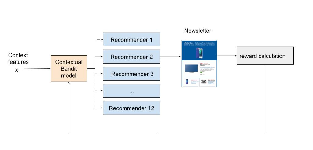
Given some features (context) about the user, and each of the 12 available recommenders, we aim to suggest best recommender (action) which increases the chance (reward) of the user clicking (reward = 1) on at least one of the recommendations by the selected recommender, and minimizes the chance of incurring a click which leads to unsubscribe (reward = -1).

By formulating the problem and reward function in this manner, we hypothesized that the system would optimize for increasing clicks, while still showing relevant (and not click-baity) content to the user in order to sustain the potential increase in performance. This is because the reward functions penalizes an event when a user unsubscribes, which a click-baity content is likely to lead to. The problem was then tackled by using contextual bandits because of the fact that they excel at exploiting trends that work well, as well as exploring and uncovering potentially even better-performing trends.

Serving millions of users every week with low latency

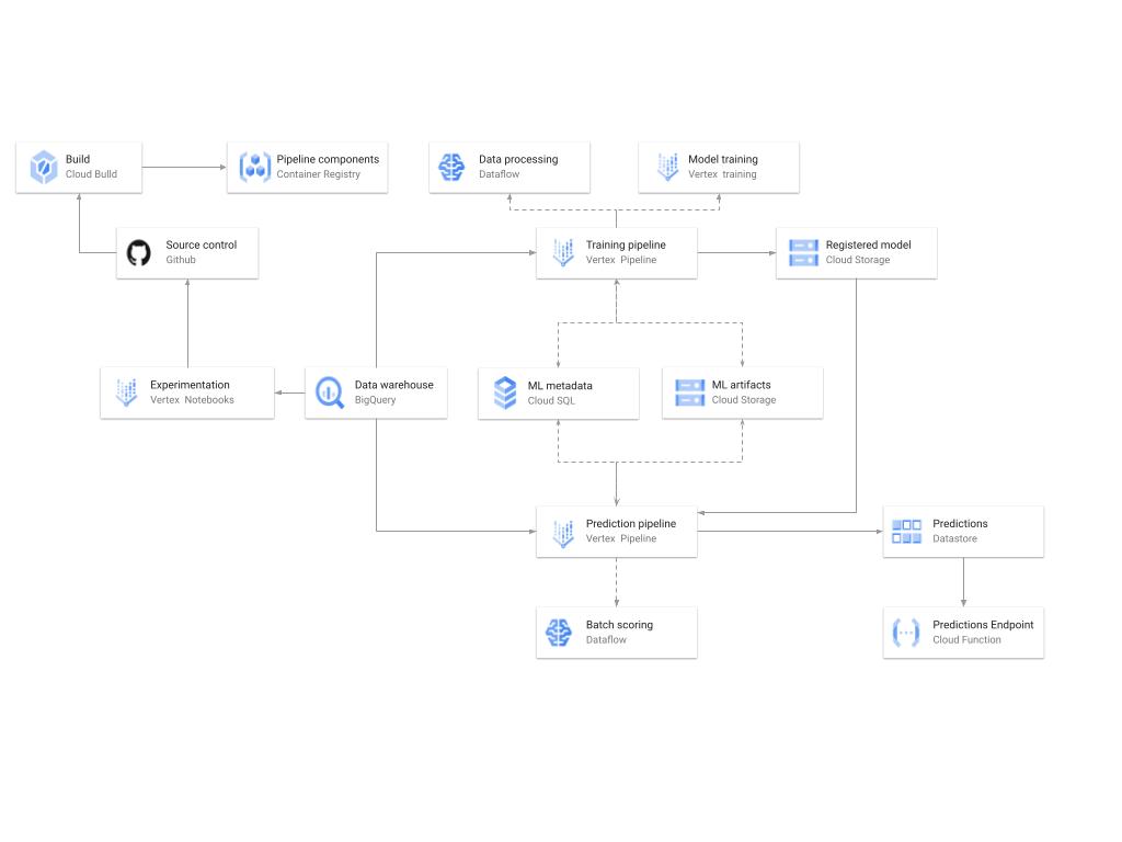A diagram showing the high-level architecture of the recommendation training and prediction systems on GCP.

There’s a lot of detail here, as the architecture shown in the diagram covers three phases of ML development, training, and serving. Here are some of the key pieces.

Model development

Vertex Notebooks are used as data science environments for experimentation and prototyping, in addition to implementing model training and scoring components and pipelines. The source code is version controlled in GitHub. A continuous integration (CI) pipeline is set up to run unit tests, build pipeline components, and store the container images to Cloud Container Registry.

Training

The training pipeline is executed using TFX on Vertex Pipelines. In essence, the pipeline trains the model using new training data extracted from BigQuery, validates the produced model, and stores it in the model registry. In our system, the model registry is curated in Cloud Storage. The training pipeline uses Dataflow for large scale data extraction, validation, processing and model evaluation, as well as Vertex Training for large scale distributed training of the model. In addition, AI Platform Pipelines stores artifacts produced by the various pipeline steps to Cloud Storage, and information about these artifacts is stored in an ML metadata database in Cloud SQL.

Serving

Predictions are produced using a batch prediction pipeline, and stored in Cloud Datastore for consumption. The batch prediction pipeline is made using TFX and runs on Vertex Pipelines. The pipeline uses the most recent model in the model registry to score the serving queries from BigQuery. A Cloud Function is provided as a REST/HTTP endpoint to retrieve predictions from Datastore.

Continuous Training Pipeline

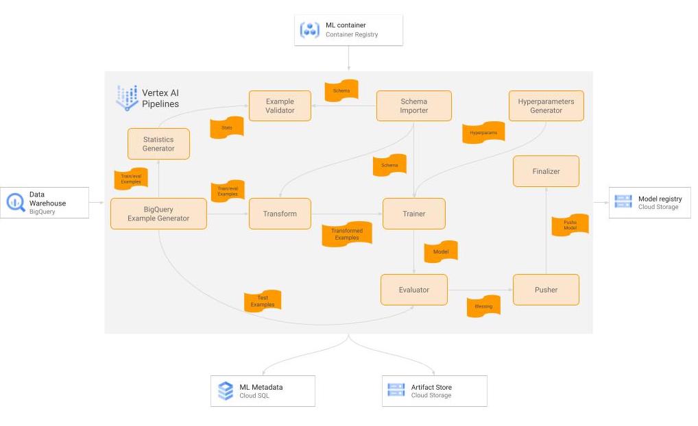A diagram of the TFX pipeline for the training workflow.

There are many components used in our TFX-based Continuous training workflow, training is currently done on an on-demand basis, but later on it is planned to be executed on a bi-weekly cadence. Here is a little bit of detail on the important ones.

Raw Data

Our data consists of multiple datasets stored in heterogeneous formats across BigQuery tables and other formats, that are then joined in denormalized fashion by the customer into a single BigQuery table for training. To help avoid bias and drift in our model we train the model on a rolling window of 4 weeks cadence with one overlapping week per training cycle. This was a simple design choice as it was very straightforward to implement, as BigQuery has good compatibility as a source with TFX, and also allows the user to do some basic data preprocessing and cleaning during fetching.

BigQueryExampleGen

We first leverage BigQuery by leveraging built-in functions to preprocess the data. By embedding our own specific processes into the query calls made by the ExampleGen component, we were able to avoid building out a separate ETL that would exist outside the scope of a TFX pipeline. This ultimately proved to be a good way to get the model in production more quickly. This preprocessed data is then split into training and eval and converted to tf.Examples via the ExampleGen component.

Transform

This component does the necessary feature engineering and transformations necessary to handle strings, fill in missing values, log-normalize values, setup embeddings etc. The major benefit here is that the resulting transformation is ultimately prepended to the computational graph, so that the exact same code is used for training and serving. The Transform component runs on Cloud Dataflow in production.

Trainer

The Trainer component trains the model using TF-Agents. We leverage parallel training on Vertex Training to speed things up. The model is designed such that the user id passes in from the input to the output unaltered, so that it can be used as part of the downstream serving pipeline. The Trainer component runs on Vertex Training in production.

Evaluator

The Evaluator compares the existing production model to the model received by the Trainer and prepares the metrics required by the validator component to bless the “better” one for use in production. The model gating criteria is based on the AUC scores as well as counterfactual policy evaluation and possibly other metrics in the future. It is easy to implement custom metrics which meet the business requirements owing to the extensibility of the evaluator component. The Evaluator runs on Vertex AI.

Pusher

The Pusher’s primary function is to send the blessed model to our TFServing deployment for production. However, we added functionality to use the custom metrics produced in the Evaluator to determine decisioning criteria to be used in serving, and attach that to the computational graph. The level of abstraction available in TFX components made it easy to make this custom modification. Overall, the modification allows the pipeline to operate without a human in the loop so that we are able to make model updates frequently, while continuing to deliver consistent performance on metrics that are important to our business.

HyperparametersGen

This is a custom TFX component which creates a dictionary with hyperparameters (e.g., batch size, learning rate) and stores the dictionary as an artifact. The hyperparameters are passed as input to the trainer.

ServingModelResolver

This custom component takes a serving policy (which includes exploration) and a corresponding eval policy (without exploration), and resolves which policy will be used for serving.

Pushing_finalizer

This custom component copies the pushed/blessed model from the TFX artifacts directory to a curated destination.

The out-of-box components from TFX provided most of the functionality we require, and it is easy to create some new custom components to make the entire pipeline satisfy our requirements. There are also other components of the pipeline such as StatisticsGen (which also runs on Dataflow).

Batch Prediction Pipeline

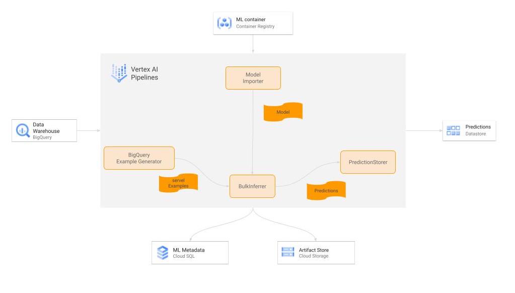A diagram showing the TFX pipeline for the batch prediction workflow.

Here are a few of the key pieces of our batch prediction system.

Inference Dataset

Our inference dataset has nearly identical format to the training dataset, except that it is emptied and repopulated with new data daily.

BigQueryExampleGen

Just like for the Training pipeline, we use this component to read data from BigQuery and convert it into tf.Examples.

Model Importer

This component imports the computation graph exported by the Pusher component of the training pipeline. As mentioned above, since it contains the whole computation graph generated by the training pipeline, including feature transformation and the tf.Agents model (including the exploration/exploitation aspect), this is very portable and prevents train/test skew.

BulkInferrer

As the name implies, this component uses the imported computation graph to perform mass inference on the inference dataset. It runs on Cloud Dataflow in production and makes it very easy to scale.

PredictionStorer

This is a custom Python Component which takes the inference results from Bulkinfererrer, post-processes them to format/filter the fields as required, and persists it to Cloud Datastore. This runs on Cloud Dataflow in production as well.

Serving is done via cloud functions which take the user ids as input, and returns the precomputed results for each userId stored in DataStore with sub 50 ms latency.

Extending the work so far

In the few months since implementation of the first version we have been making dozens of improvements to the pipeline, everything from changing the architecture/approach of the original model, to changing the way the model’s results are used in the downstream application to generate newsletters. Moreover, each of these improvements brings new value to us more quickly than we’ve been able to in the past.

Since our initial implementation of this reference architecture, we have released a simple Vertex AI pipeline based github code samples to implementing recommender systems using TF Agents here. By using this template and guide, it will help them build recommender systems using contextual bandits on GCP in a scalable, modularized, low latency and cost effective manner. It’s quite remarkable how many of the existing TFX components that we have in place carry over to new projects, and even more so how drastically we’ve reduced the time it takes to get a model in production. As a result, even the software engineers on our team without much ML expertise feel confident in being able to reuse this architecture and adapt it to more use cases. The data scientists are able to spend more of their time optimizing the parameters and architectures of the models they produce, understanding their impact on the business, and ultimately delivering more value to the users and the business.

Acknowledgements

None of this would have been possible without the joint collaboration of the following Googlers: Khalid Salama, Efi Kokiopoulou, Gábor Bartók and Digitec Galaxus’s team of engineers.

A Google Cloud blog on this project can be found here.

Read More

Posted by Gábor Bartók and Efi Kokiopoulou, Google Research

This article assumes you have some prior experience with reinforcement learning and/or multi-armed bandits. If you’re new to the subject, a good starting point is the Bandits Wikipedia entry, or for a bit more technical and in-depth introduction, this book.

In this blog post we introduce the TensorFlow-Agents Bandits library. This library offers a comprehensive list of the most popular bandit algorithms along with a variety of test problems on which the algorithms can be run. The test problems (called bandit environments) include some synthetic environments as well as environments converted from real-life (classification or recommendation) datasets.

One of the latter is the MovieLens environment, which utilizes this dataset. In this blog post, we will guide you through the usage of the TF-Agents Bandits library with the help of the MovieLens Environment.

Multi-Armed Bandits

Multi-Armed Bandits is a machine learning framework in which an agent repeatedly selects actions from a set of actions and collects rewards by interacting with the environment. The goal of the agent is to accumulate as much reward as possible, within a given time horizon. The name “bandit” comes from the illustrative example of finding the best slot machine (one-armed bandit) from a set of machines with different payoffs. The actions are also known as “arms”.

Image from Wikipedia

There are two more important concepts to be aware of: “context”, and “regret”. In many real life scenarios, it’s not enough to find the best action that on average provides the highest reward: we want to find the best action depending on the situation/context. To extend the bandits framework in this direction, we introduce the notion of “context”. Before the agent has to select an action, it receives the context that provides information about the current round. Then the agent’s goal is to find the policy that selects the highest-rewarding action for the given context.

In bandits literature, the notion of “regret” is very important. The regret can be informally defined as the difference in performance between the optimal policy and the learned policy. Typically the performance is measured in terms of cumulative reward (i.e., sum of rewards across several rounds); otherwise, one may also refer to the “instantaneous regret” which is the regret the agent suffers at a certain round. Bandit algorithms typically come with performance guarantees in terms of upper bound on the regret given a family of bandit problems.

Example: Movie Recommendation

Consider the following scenario. You are tasked with recommending movies to users of a movie streaming service. In every round you receive information about the user. Your task is to choose from a handful of movies for the user with the goal of choosing one that the user will enjoy and give a high rating.

A Recommendation Dataset

For illustration purposes, we will turn the well-known MovieLens dataset into a bandit problem. The dataset consists of ~100K ratings from 943 users on 1682 movies. Our first step to turn this dataset into a contextual bandit problem is to construct the matrix `A` of user/movie ratings, where `A_ij` is the rating of user `i` of movie `j`. Since we have the ratings to a few movies only from each user, one issue with the ratings matrix `A` is that it is very sparse i.e., only a few entries `A_ij` are available; all the other entries are unknown. To address this sparsity issue, we construct a low-rank SVD decomposition `A ~= U*V’` (low-rank matrix decomposition in recommender systems is a popular approach for collaborative filtering, see e.g., Koren et al. 2009). This way, the rows of `U` are context features. Then, the movies to be recommended to the user are the set of actions, represented as rows of `V`. The reward for recommending movie `j` to user `i` can then be calculated as the inner product of the corresponding rows of `U_i` and `V_j`. Therefore, using the low-rank SVD decomposition to compute rewards gives us the ability to approximate the reward even for movies that were not recommended to the users; hence their rating was unknown.

TF-Agents Bandits

Now let’s see how the above problem is modeled and solved with the help of the TF-Agents Bandits library. TF-Agents is a modular library that has building blocks for every aspect of Reinforcement Learning and Bandits. A problem can be expressed in terms of an “environment”. An environment is a class that generates observations (aka contexts), and also outputs a reward after being presented with actions. In the case of the MovieLens environment, an observation is a random row of the matrix `U`, while the reward is given after an algorithm has chosen an action (i.e., row of the matrix `V`, a movie in our case). The implementation of the MovieLens environment can be found here. It’s worth noting here that it is rather simple to implement a bandit environment in TF-Agents. For a walkthrough, we refer the reader to our Bandits Tutorial.

Algorithms

Bandit algorithms in TF-Agents have two main building blocks: “policies” and “agents”. A policy is a function that, given an observation, chooses an action. The agent is responsible for learning a good policy: given examples of (observation, action, reward) tuples, it trains the policy so that it chooses better actions. The TF-Agents Bandits library offers a comprehensive list of the most popular algorithms, including linear methods as well as nonlinear ones (e.g., those with neural network-based value functions). Let’s see how LinUCB tackles the MovieLens problem!

The LinUCB algorithm

In short, the LinUCB algorithm keeps track of running average rewards for all actions, along with confidence intervals around the estimates. In every turn, the algorithm chooses the action that has the highest upper confidence bound on its reward estimate.

In the TF-Agents library, the LinUCB algorithm is built from a LinearBanditPolicy with an “Optimistic Exploration Strategy”, and a LinearBanditAgent responsible for updating the estimates. Note that the exploration strategy can be changed from “Optimistic” to “Sampling”, in which case the algorithm becomes Linear Thompson Sampling.

So let’s see how LinUCB performs on the MovieLens environment! We ran LinUCB on the MovieLens environment (with 100 actions and SVD decomposition rank 20) and we get results on TensorBoard:

(Note that all of the below plots are based on averaging five runs, the shadows show standard deviations. A rolling average smoothing is also applied on the curves.)

Linear Thompson Sampling

As mentioned above, with a slight modification of LinUCB, we get an implementation for Linear Thompson Sampling (LinTS). If we run LinTS on the same problem (implementation here), we get a very similar result to that of LinUCB (see joint graph further down).

NeuralEpsilonGreedy

Let’s compare these results with another agent, say, the NeuralEpsilonGreedy agent. As the name suggests, this agent uses a neural network to estimate the rewards, and adds uniform exploration with probability `epsilon`. This exploration strategy is known as “epsilon-greedy” since the method is greedy most of the time but with probability `epsilon` it explores by picking an action uniformly at random. If we run Neural Epsilon Greedy and put the results from the three algorithms, we get:

It’s interesting to also look at how often the methods pick suboptimal actions. This is shown below:

We see that LinUCB and LinTS have very similar performance, which is not very surprising, as they are very similar algorithms. On the other hand, Neural epsilon-Greedy is not doing very well on this problem. After fifty thousand iterations, the metrics are still far away from that of the linear methods. Note, nevertheless, that even the epsilon-Greedy algorithm manages to find the best movie about half the time, out of 100, still not bad!

To be fair, it’s expected that linear algorithms do better than non-linear ones on this problem, as the problem is linear (by the reward calculation construction).

As for the difference between the two linear algorithms, it seems that LinUCB struggles in the beginning a little bit, but in the long run it is slightly (not significantly) better than LinTS.

Recommendation with Arm Features

The MovieLens example above has some shortcomings: its actions are a selection of movies, algorithms have to learn a distinct model for every movie, and it’s also hard to introduce new movies in the system. To this end, we change the environment a little bit: instead of treating every movie as an independent action, we model the movies with features, similarly to users: the rows of `V` will be the movie features. Then the model only has to learn one reward function, whose input is both the user features `u` and the movie features `v`. This way we can have an unlimited number of movies in the system, and we can introduce new movies on the fly. This version of the environment can be found here.

Agents Running on Per Arm Feature Environments

Most of the agents implemented in our library have the functionality of running on environments that have features for its actions (we call these environments “per-arm environments”).

Now let’s see how the different algorithms behave on the per-arm version of the MovieLens environment. We ran the arm-feature versions of the three algorithms: LinUCB, LinTS, and eps-Greedy. The result is quite different from the previous section: Here the linear methods seem to fail to find the relationship between actions and rewards, while the neural approach gives similar results to that of the non-arm feature problem.

The neural algorithm still finds the best action ~45% of the time, while the linear algorithms only ~30% of the time.

Your New Bandit Algorithm

If you haven’t found what you are looking for in the list of agents within the library, it’s possible, and not too complicated, to implement your own algorithm. You need to:

• subclass tf_agents.policies.TFPolicy and
• subclass tf_agents.agents.TFAgent.

TFPolicy

To define a policy, one needs to implement its private member function _distribution(…). In short, this function takes an observation and outputs a distribution of actions (or simply an action in case of a deterministic policy).

TFAgent

As stated above, an agent is responsible for training the policy. To this end, subclasses of TF-Agents’ TFAgent (sorry) have to implement the private member function _train() (among others, some details are omitted for clarity). This function takes batches of training data, and trains the policy.

Your New Bandit Environment

If you want to test your (new) algorithm and have an idea for an environment, it’s also simple to implement it in TF-Agents. A Bandit environment has two main roles: (i) to generate observations, and (ii) to return a reward after the agent chooses an action. One can easily create an environment class by defining these two functions.

Recap

In this blog post, we introduced the TF-Agents Bandit library and showed how to tackle a recommendation problem with it. If you want to play around with the environments and agents used in this post, you can go directly to this executable to run these agents and more. If you want to explore the library or just want to read more about it, we suggest starting with this tutorial. And if you’re interested in learning more about making recommendations on this MovieLens dataset, you can also check out another great library called TensorFlow Recommenders.

Collaborators

The TF-Agents Bandits library has been built in collaboration with Jesse Berent, Tzu-Kuo Huang, Kishavan Bhola, Sergio Guadarrama‎, Anoop Korattikara, Oscar Ramirez, Eugene Brevdo, and many others from the TF-Agents team.

Read More

Posted by Yunlu Li and Artsiom Ablavatski

Introduction

Pruning is one of the core optimization techniques provided in the TensorFlow Model Optimization Toolkit (TF MOT). Not only does it help to significantly reduce model size, but it can also be used to accelerate CPU inference on mobile and web. With modern compute intensive models, the area of pruning as a model optimization technique has drawn significant attention, demonstrating that dense networks can be easily pruned (i.e. a fraction of the weights set to zero) with negligible quality degradation. Today, we are excited to announce a set of updates to TF MOT Pruning API that simplify pruning and enable developers to build sparse models for fast on-device inference.

Updates to TF MOT

TensorFlow has long standing support for neural network pruning via TensorFlow Model Optimization Toolkit (TF MOT) Pruning API. The API, featured in 2019, introduced essential primitives for pruning, and enabled researchers throughout the world with new optimization techniques. Today we are happy to announce experimental updates to the API that further advance model pruning. We are releasing tools that simplify the control of pruning and enable latency reduction for on-device inference.

The TF MOT Pruning API has extensive functionality that provides the user with tools for model manipulation:

• prune_low_magnitude function applies PruneLowMagnitude wrapper to every layer in the model
• PruneLowMagnitude wrapper handles low-level pruning logic
• PruningSchedule controls when pruning is applied
• PruningSummaries callback logs the pruning progress

These abstractions allow to control almost any aspect of model pruning (i.e. how to prune (PruneLowMagnitude), when to prune (PruningSchedule) and how to track the progress of the pruning (PruningSummaries) with the exception of what to prune, i.e. where PruneLowMagnitude wrapper is applied. We are happy to release an extension of TF MOT PruningPolicy, a class that controls which parts of the model the PruneLowMagnitude wrapper is applied to. The instance of PruningPolicy is used as an argument in the prune_low_magnitude function and provides the following functionalities:

• Controls where the pruning wrapper should be applied on per-layer basis through the allow_pruning function
• Checks that the whole model supports pruning via ensure_model_supports_pruning function

PruningPolicy is an abstract interface, and it can have many implementations depending on the particular application. For latency improvements on CPU via XNNPACK, the concrete implementation PruneForLatencyOnXNNPack applies the pruning wrapper only to the parts of the model that can be accelerated via sparse on-device inference while leaving the rest of the network untouched. Such selective pruning allows an application to maintain model quality while targeting parts of the model that can be accelerated by sparsity.

The below example showcases the PruneForLatencyOnXNNPack policy in action on

MobileNetV2 (the full example is available in a recently introduced colab):

import tensorflow as tf
import tensorflow_model_optimization as tfmot
prune_low_magnitude = tfmot.sparsity.keras.prune_low_magnitude

# See the implementation of the function below.
model = load_model_for_pruning()

model_for_pruning = prune_low_magnitude(
    model, pruning_policy=tfmot.sparsity.keras.PruneForLatencyOnXNNPack())

In order to comply with the constraints of XNNPACK sparse inference the Keras implementation of MobileNetV2 model requires slight modification of the padding for the first convolution operation:

def load_model_for_pruning():
  input_tensor = tf.keras.layers.Input((224, 224, 3))
  input_tensor = tf.keras.layers.ZeroPadding2D(1)(input_tensor)
  model = tf.keras.applications.MobileNetV2(input_tensor=input_tensor)

  def clone_fn(layer):
    if layer.name == 'Conv1':
      # The default padding `SAME` for the first convolution is incompatible
      # with XNNPACK sparse inference.
      layer.padding = 'valid'
      # We ask the model to rebuild since we've changed the padding parameter.
      layer.built = False
    return layer

  return tf.keras.models.clone_model(model, clone_function=clone_fn)

The PruneForLatencyOnXNNPack policy applies the pruning wrapper only to convolutions with 1×1 kernel size since only these layers can be accelerated on CPU by as much as 2x using XNNPACK. The rest of the layers are left untouched allowing the network to recover after quality degradation at the pruning step. Also, the policy verifies that the model is amenable to being pruned by using the ensure_model_supports_pruning method. Once the sparse model has been trained and converted, we recommend using the TensorFlow Lite benchmark utility in debug mode to confirm that the final model is compatible with XNNPack’s sparse inference backend.

We hope that this newly introduced experimental API will be useful in practice and we will continue to improve its stability and flexibility in the future.

Compression and Latency Improvements

Model compression is another major benefit of applying pruning to a model. Using a smart compression format allows efficient storage of model weights which leads to a significant size reduction.

TFLite adopted the TACO format to encode sparse tensors. Compared to widely used formats like CSR and CSC, the TACO format has several advantages:

1. It supports flexible traversal order to store a tensor in row-major or column-major formats easily.
2. It supports multi-dimensional sparse tensors like the 4-D filter of a convolution op.
3. It can represent block structure as the inner dimension of the tensor (example of a 4×4 tensor with 2×2 inner block structure).

We also adapted the format to use flexible data types for the metadata storing the indices of non-zero elements. This reduces the storage overhead for small tensors, or tensors with compact data types like int8_t.

In order to realize size reductions in practice during the model conversion, the tf.lite.Optimize.EXPERIMENTAL_SPARSITY optimization needs to be applied. This optimization handles examining the model for sparse tensors and converting them to an efficient storage format. It also works seamlessly with quantization and you can combine them to achieve more aggressive model compresion. The full example of such a conversion is shown below:

# Remove the pruning wrappers from the model. 
model = tfmot.sparsity.keras.strip_pruning(model)

converter = tf.lite.TFLiteConverter.from_keras_model(model)
# We apply float16 quantization together with sparsity optimization that
# compactly stores pruned weights.
converter.optimizations = [
    tf.lite.Optimize.EXPERIMENTAL_SPARSITY,  # Enables size reduction optimization. 
    tf.lite.Optimize.DEFAULT  # Enables quantization at conversion.
]
converter.target_spec.supported_types = [tf.float16]
tflite_buffer = converter.convert()

After applying the tf.lite.Optimize.EXPERIMENTAL_SPARSITY optimization together with PruneForLatencyOnXNNPack pruning policy, a ~2x size reduction can be achieved as is demonstrated in Figure 1:

Figure 1. Ablation study of MobileNetV2 model size (float32 and float16 types) with different sparsity levels using PruneForLatencyOnXNNPack pruning policy. Only the 1×1 convolutional layers are pruned and the rest of the layers are left dense.

In addition to size reduction, pruning can provide inference acceleration on CPU via XNNPACK. Using the PruneForLatencyOnXNNPack pruning policy, we’ve conducted an ablation study of CPU inference latency for a MobileNetV2 model on Pixel 4 using TensorFlow Lite benchmark with the use_xnnpack option enabled:

Figure 2. Ablation study of CPU inference speed of MobileNetV2 model with different sparsity levels on a Pixel 4 device.

This study in Figure 2 demonstrates 1.7x latency improvement when running on mobile devices using XNNPACK. The strategies for training the sparse MobileNetV2 model together with hyperparameters and pre-trained checkpoints are described in Elsen et al.

Pruning techniques & tips

Pruning aware training is a key step in model optimization. Many hyperparameters are involved in training and some of them like the pruning schedule and learning rate can have a dramatic impact on the final quality of the model. Though many strategies have been proposed, a simple yet effective 3-steps strategy (see Table 1) achieves strong performance for the majority of our use cases. The strategy builds on top of the well-proven approach from Zhu & Gupta and produces good results without extensive re-training:

The strategy inevitably leads to a substantial increase (~3x) in the training time. However, paired with the PolynomialDecay pruning schedule, this 3-step strategy achieves limited or no quality degradation with significantly pruned (>70%) neural networks.

Pruned models in MediaPipe

Together with the updates to the TF MOT Pruning API, we are happy to release pruned models for some of the MediaPipe solutions. The released models include pose and face detectors as well as a pruned hand tracking model. All of these models have been trained with the newly introduced functionality using the 3-steps pruning strategy. Compared with dense baselines the released pruned models have demonstrated significant model size reduction as well as superior performance when running on CPU via XNNPACK. Quality-wise the pruned models achieve similar metrics including in the evaluation on our fairness datasets (see model cards for details). Side-by-side demos of the solutions are shown below:

Figure 3. Comparison of dense (left) and sparse (right) models in the end-to-end examples of face (top) and pose (bottom) detection

Pruning for GPU

While exploiting sparsity on GPUs can be challenging, recent work has made progress in improving the performance of sparse operations on these platforms. There is momentum for adding first-class support for sparse matrices and sparse operations in popular frameworks, and state-of-the-art GPUs have recently added hardware acceleration for some forms of structured sparsity. Going forward, improvements in software and hardware support for sparsity in both training and inference will be a key contributor to progress in the field.

Future directions

TF MOT offers a variety of model optimization methods, many of which have proven to be essential for efficient on-device model inference. We will continue to expand the TF MOT Pruning API with algorithms beyond low magnitude pruning, and also investigate the combination of pruning and quantization techniques to achieve even better results for on-device inference. Stay tuned!

Acknowledgments

Huge thanks to all who worked on this project: Karthik Raveendran, Ethan Kim, Marat Dukhan‎, Trevor Gale, Utku Evci, Erich Elsen, Frank Barchard, Yury Kartynnik‎, Valentin Bazarevsky, Matsvei Zhdanovich, Juhyun Lee, Chuo-Ling Chang, Ming Guang Yong, Jared Duke‎ and Matthias Grundmann.

Read More

Posted by Michael Brooks, Coral

For over 3 years, Coral has been focused on enabling privacy-preserving Edge ML with low-power, high performance products. We’ve released many examples and projects designed to help you quickly accelerate ML for your specific needs. One of the most common requests we get after exploring the Coral models and projects is: How do we move to production?

With this in mind we’re introducing the first of our use-case specific demos. These demos are intended to to take full advantage of the Coral Edge TPU™ with high performance, production-quality code that is easily customizable to meet your ML requirements. In this demo we focus on use cases that are specific to manufacturing; worker safety and quality grading / visual inspection.

Demo Overview

The Coral manufacturing demo targets a x86 or powerful ARM64 system with OpenGL acceleration that processes and displays two simultaneous inputs. The default demo, using the included example videos, looks like this:

The two examples being run are:

• Worker Safety: Performs generic person detection (powered by COCO-trained SSDLite MobileDet) and then runs a simple algorithm to detect bounding box collisions to see if a person is in an unsafe region.
• Visual Inspection: Performs apple detection (using the same COCO-trained SSDLite MobileDet from Worker Safety) and then crops the frame to the detected apple and runs a retrained MobileNetV2 that classifies fresh vs rotten apples.

By combining these two examples, we are able to demonstrate multiple Coral features that can enable this processing, including:

• Co-compilation
• Cascading models (using the output of one model to feed another)
• Classification retraining
• Real time processing of multiple inputs

Creating The Demo

When designing a new ML application, it is critical to ensure that you can meet your latency and accuracy requirements. With the two applications described here, we went through the following process to choose models, train these models, and deploy to the EdgeTPU – this process should be used when beginning any Coral application.

Choosing the Models

When deciding on a model to use, the new Coral Model Page is the best place to start. For this demo, we know that we need a detection model (which will be used for detection of both people and apples) as well as a classification model.

Detection

When picking a detection model from the Detection Model Page, there are four aspects to a model we want to look for:

1. Training Dataset: In the case of the models page, all of our normal detection models use the COCO dataset. Referring to the labels, we can find both apples and people, so we can use just the one model for both detection tasks.
2. Latency: We will need to run at least 3 inferences per frame and need this to keep up with our input (30 FPS). This means we need our detection to be as fast as possible. From the models page, we can see two good options: SSD MobileNet v2 (7.4 ms) and MobileDet (8.0 ms). This is the first point where we see the clear advantage of Coral – looking at the benchmarks at the bottom of our x86+USB CTS Output we can see even on a powerful workstation this would be 90 ms and 123 ms respectively.
3. Accuracy/Precision: We also want as accurate a model as possible. This is evaluated using the primary challenge metric from COCO evaluation metrics. We see here MobileDet (32.8%) clearly outpeforms MobileNet V2 (25.7%).
4. Size: In order to fully co-compile this detection model with the classification model below, we need to ensure that we can fit both models in the 8MB of cache on the Edge TPU. This means we want as small a model as possible. MobileDet is 5.1 MB vs MobileNet V2 is 6.6 MB.

With the above considerations, we chose SSDLite MobileDet.

Classification

For the fresh-or-rotten apple classification, there are many more options on the Coral Classification Page. What we want to check is the same:

1. Training Dataset: We’ll be retraining on our new dataset, so this isn’t critical in this application.
2. Latency: We want the classification to be as fast as possible. Luckily many of the models on our page are extremely fast relative to the 30 FPS frame rate we demand. With this in mind we can eliminate all the Inception models and ResNet-50.
3. Accuracy: Accuracy for Top-1 and Top-5 is provided. We want to be as accurate as possible for Top-1 (since we are only checking fresh vs rotten) – but still need to consider latency. With this in mind we eliminate MobileNet v1.
4. Size: As mentioned above, we want to ensure we can fit both the detection and classification models (or as much as possible) so we can easily eliminate the EfficientNet options.

This leaves us with MobileNet v2 and MobileNet v3. We opted for v2 due to existing tutorials on retraining this model.

Retraining Classification

With the model decisions taken care of, now we need to retain the classification model to identify fresh and rotten apples. Coral.ai offers training tutorials in CoLab (uses post-training quantization) and Docker (uses quantization aware training) formats – but we’ve also included the retraining python script in this demo’s repo.

Our Fresh/Rotten data comes from the “Fruits fresh and rotten for classification” dataset – we simply omit everything but apples.

In our script, we first load the standard Keras MobileNetV2 – freezing the first 100 layers and adding a few extra layers at the end:

base_model = tf.keras.applications.MobileNetV2(input_shape=input_shape,
                                                    include_top=False,
                                                    classifier_activation='softmax',
                                                    weights='imagenet')
# Freeze first 100 layers
base_model.trainable = True
for layer in base_model.layers[:100]:
  layer.trainable = False
model = tf.keras.Sequential([
    base_model,
    tf.keras.layers.Conv2D(filters=32, kernel_size=3, activation='relu'),
    tf.keras.layers.Dropout(0.2),
    tf.keras.layers.GlobalAveragePooling2D(),
    tf.keras.layers.Dense(units=2, activation='softmax')
])
model.compile(loss='categorical_crossentropy',
              optimizer=tf.keras.optimizers.RMSprop(lr=1e-5),
              metrics=['accuracy'])
print(model.summary())

Next, with the dataset download into ./dataset we train our model:

train_datagen = ImageDataGenerator(rescale=1./255,
                                   zoom_range=0.3,
                                   rotation_range=50,
                                   width_shift_range=0.2,
                                   height_shift_range=0.2,
                                   shear_range=0.2,
                                   horizontal_flip=True,
                                   fill_mode='nearest')
val_datagen = ImageDataGenerator(rescale=1./255)
dataset_path = './dataset'
train_set_path = os.path.join(dataset_path, 'train')
val_set_path = os.path.join(dataset_path, 'test')
batch_size = 64
train_generator = train_datagen.flow_from_directory(train_set_path,
                                                    target_size=input_size,
                                                    batch_size=batch_size,
                                                    class_mode='categorical')
val_generator = val_datagen.flow_from_directory(val_set_path,
                                                target_size=input_size,
                                                batch_size=batch_size,
                                                class_mode='categorical')
epochs = 15
history = model.fit(train_generator,
                    steps_per_epoch=train_generator.n // batch_size,
                    epochs=epochs,
                    validation_data=val_generator,
                    validation_steps=val_generator.n // batch_size,
                    verbose=1)

Note that we’re only using 15 epochs. When retraining on another dataset it is very likely more will be required. With the apple dataset, we can see this model quickly hits very high accuracy numbers:

For your own dataset and model more epochs will likely be needed (the script will generate the above plots for validation).

We now have a Keras model that works for our apple quality inspector. In order to run this on a Coral Edge TPU, the model must be quantized and converted to TF Lite. We’ll do this using post-training quantization – quantizing based on a representative dataset after training:

def representative_data_gen():
  dataset_list = tf.data.Dataset.list_files('./dataset/test/*/*')
  for i in range(100):
    image = next(iter(dataset_list))
    image = tf.io.read_file(image)
    image = tf.io.decode_jpeg(image, channels=3)
    image = tf.image.resize(image, input_size)
    image = tf.cast(image / 255., tf.float32)
    image = tf.expand_dims(image, 0)
    yield [image]
model.input.set_shape((1,) + model.input.shape[1:])
converter = tf.lite.TFLiteConverter.from_keras_model(model)
converter.optimizations = [tf.lite.Optimize.DEFAULT]
converter.representative_dataset = representative_data_gen
converter.target_spec.supported_ops = [tf.lite.OpsSet.TFLITE_BUILTINS_INT8]
converter.target_spec.supported_types = [tf.int8]
converter.inference_input_type = tf.uint8
converter.inference_output_type = tf.uint8
tflite_model = converter.convert()

The script will then compile the model and evaluate both the Keras and TF Lite models – but we’ll need to take one extra step beyond the script: We must use the Edge TPU Compiler to co-compile the classification model with our detection model.

Co-compiling the models

We now have two quantized TF Lite models: classifier.tflite and the default CPU model for MobileDet taken from the Coral model page. We can compile them together to ensure that they share the same caching token – when either model is requested the parameter data will already be cached. This simply requires passing both models to the compiler:

edgetpu_compiler ssdlite_mobiledet_coco_qat_postprocess.tflite classifier.tflite 
Edge TPU Compiler version 15.0.340273435

Models compiled successfully in 1770 ms.

Input model: ssdlite_mobiledet_coco_qat_postprocess.tflite
Input size: 4.08MiB
Output model: ssdlite_mobiledet_coco_qat_postprocess_edgetpu.tflite
Output size: 5.12MiB
On-chip memory used for caching model parameters: 4.89MiB
On-chip memory remaining for caching model parameters: 2.74MiB
Off-chip memory used for streaming uncached model parameters: 0.00B
Number of Edge TPU subgraphs: 1
Total number of operations: 125
Operation log: ssdlite_mobiledet_coco_qat_postprocess_edgetpu.log

Model successfully compiled but not all operations are supported by the Edge TPU. A percentage of the model will instead run on the CPU, which is slower. If possible, consider updating your model to use only operations supported by the Edge TPU. For details, visit g.co/coral/model-reqs.
Number of operations that will run on Edge TPU: 124
Number of operations that will run on CPU: 1
See the operation log file for individual operation details.

Input model: classifier.tflite
Input size: 3.07MiB
Output model: classifier_edgetpu.tflite
Output size: 3.13MiB
On-chip memory used for caching model parameters: 2.74MiB
On-chip memory remaining for caching model parameters: 0.00B
Off-chip memory used for streaming uncached model parameters: 584.06KiB
Number of Edge TPU subgraphs: 1
Total number of operations: 72
Operation log: classifier_edgetpu.log
See the operation log file for individual operation details.

There are two things to note in this log. First is that we see one operation is run on the CPU for the detection model – this is expected. The TF Lite SSD PostProcess will always run on CPU. Second, we couldn’t quite fit everything on the on-chip memory, the classifier has 584 kB of off-chip memory needed. This is fine – we’ve substantially reduced the amount of IO time needed. Both models will now be in the same folder, but because we co-compiled them they are aware of each other and the cache will persist parameters for both models.

Customizing For Your Application

The demo is optimized and ready for customization and deployment. It can be cross compiled for other architectures (currently it’s only for x86 or ARM64) and statically links libedgetpu to allow this binary to be deployed to many different Linux systems with an Edge TPU.

There are many things that can be done to customize the model to your application:

• The quickest changes are the inputs, which can be adjusted via the --visual_inspection_input and --worker_safety_input flags. The demo accepts mp4 files and V4L2 camera devices.
• The worker safety demo can be further improved with more complicated keepout algorithms (including consideration of angle/distance from camera) as well as retraining on overhead data. Currently the demo checks only the bottom of the bounding box, but the flag --safety_check_whole_box can be used to compare to the whole box (for situations like overhead cameras).
• The apple inspection demonstrates simple quality grading / inspection – this cascaded model approach (using detection to determine bounding boxes and feeding into another model) can be applied to many different uses. By retraining the detection and classification model this can be customized for your application.

Conclusion

The Coral Manufacturing Demo demonstrates how Coral can be used in a production environment to solve multiple ML needs. The Coral accelerator provides a low-cost and low-power way to add enough ML compute to run both tasks in parallel without over-burdening the host. We hope that you can use the Coral Manufacturing Demo as a starting point to bringing Coral intelligence into your own manufacturing environment.

To learn more about ways edge ML can be used to benefit day to day operations across a variety of industries, visit our Industries page. For more information about Coral Products and Partner products with Coral integrated, please visit us at Coral.ai.

Read More

Posted by Alina Shinkarsky and Jocelyn Becker on behalf of the TensorFlow Team

The TensorFlow Developer Certificate exam is celebrating its first anniversary with a big milestone: more than 3,000 people have passed the exam! Successful test takers received the official TensorFlow Developer Certificate and badge. They also had the opportunity to showcase their skill set on social networks such as LinkedIn and the TensorFlow Certificate Network, where recruiters are able to seek out entry-level TensorFlow developers.

The goal of this program is to provide developers around the world with the opportunity to demonstrate their skills in ML in an increasingly AI-driven global job market. This is a foundational certificate for students, developers, and data scientists who want to demonstrate practical machine learning skills through building and training basic models using TensorFlow.

We’ve followed up with folks who have taken the exam to understand the impact on their professional lives.

Fran shared, “Lost my job due to COVID 1 month before taking the exam, hired by Google in August, I think this cert helped a lot for my resume to be selected for interviews :)“

Fran is now a Conversational AI engineer, and has been working at Google for over 6 months.

Tia shared, “I was a stay-at-home mom when I started to learn Machine Learning at Google Bangkit Academy back in 2020. Bangkit supported us to take TF Certification and with this certificate, I was able to get back to work after years of hiatus. My current role is Machine Learning Curriculum Developer in Dicoding, an online technology education platform in Indonesia.”

Check out the short video below to hear Tia’s story.

Are you interested in earning the TensorFlow Developer Certificate? Learn more about the TensorFlow Developer Certificate on our website, including information on exam criteria, exam cost, and a stipend application to ensure taking this certificate exam is accessible, regardless of income.

If you’ve taken the exam and have feedback or would like to share your story, we would love to hear from you!

We look forward to growing this community of TensorFlow Developer Certificate recipients, and are immensely thankful to the continued contributions of our open source community!

Note: Participating in the program and/or obtaining this certificate are not endorsements of a participant’s employability nor guarantee of future work performance.

Read More

Posted by Luiz GUStavo Martins and Elizabeth Kemp on behalf of the TensorFlow Hub team

As a developer, when you’re faced with a challenge, you might think: “How can I solve this?”, or, “What is the right tool for the job?” For a growing number of situations, machine learning can help! ML can solve many tasks that would be very challenging using classical programming, for example: detecting objects in images, classifying sound events, or understanding text.

But training machine learning models may take a lot of time, use large amounts of data, require deep expertise in the field, and be resource intensive. What if instead of starting from scratch, someone has already solved the same problem you have? Or at least solved a very similar problem that could give you a good starting point? This is where TensorFlow Hub can help you!

TensorFlow Hub is an open repository of pre-trained machine learning models ready for fine-tuning and deployable anywhere, from servers to mobile devices, microcontrollers and browsers.

Developers are using models available from TF Hub to solve real world problems across many domains, and at Google I/O 2021 we highlighted some examples of developers changing the world using models from TensorFlow Hub.

In this article, we’ll cover these use cases as well, with links so you can check them out.

Images

Image classification is one of the most popular use cases for machine learning. The development of this field helped the whole of machine learning by showing very good results and pushing the boundaries of research.

TensorFlow Hub has many models for the image problem domain for tasks like image classification, object detection, image segmentation, pose detection, style transfer and many others.

Many of the available models have a visualizer, like the one below, right on their documentation page, enabling you to try the model without any code or downloading anything.

TFHub makes Transfer Learning simpler and easier to experiment with many state of the art models like MobilenetV3, EfficientNet V2 to find the best one for your data. A real world use case can be seen in this CropNet tutorial to create the best model possible to detect diseases in cassava leaves and deploy it on device for use in the field.

Text

Understanding text has always been a very challenging task for computers because of all the context that is necessary, and the large number of words and phrases. Many state of the art Natural Language Processing (NLP) models are available on TensorFlow Hub and ready for you to use.

One example is the BERT family of models. Using them from TFHub is easier than ever. Aside from the base BERT model, there are more advanced versions and in many languages ready to be used like you can see here in Making BERT Easier with Preprocessing Models From TensorFlow Hub.

One good example is the MuRIL model that is a multilingual BERT model trained on 17 Indian languages used by developers to solve local NLP challenges in India.

An animation of the preprocessing model that makes it easy for you to input text into BERT.

Developers can also use the TF Hub spam detection model for detecting spam comments in online forums. The model is available for TF.js and TFLite for running in the browser and on-device.

Audio

TF Hub has many audio models that you can use on desktop, for on-device inference on mobile devices, or on the web. There are also audio embedding models that can be used with transfer learning which you can adapt to your own data.

Developers are using audio classification to understand what’s happening on a forest (How ZSL uses ML to classify gunshots to protect wildlife) or inside the ocean (Acoustic Detection of Humpback Whales Using a Convolutional Neural Network) or even closer to us, understanding what is happening in your own home (Important household sounds become more accessible).

Video

Video processing is increasingly important and TensorFlow Hub also has models for this domain like the MoViNet collection that can do video classification or the I3D for action recognition.

TFHub also has tutorials for Action recognition, Video Interpolation and Text-to-video retrieval.

Summary

Reusing code is usually better than re-writing it. The same applies to machine learning models. If you can use a pre-trained model for a task, it can save you time, resources, and help you make an impact in the world. TensorFlow Hub has thousands of models available for you to deploy or customize to your task with transfer learning.

If you want to know more about how to use TensorFlow Hub and find great tutorials, check out the documentation at tensorflow.org/hub. To find models for your own real world impact, search on tfhub.dev.

Let us know what you build and also share with the community. You can talk to the team on the TensorFlow Forum and find a community that is eager to help!

Read More

Cross posted with the Google Cloud blog by Tao Wang, Software Engineer, Aarush Selvan, Product Manager.

The latest round of MLPerf benchmark results have been released, and Google’s TPU v4 supercomputers demonstrated record-breaking performance at scale. This is a timely milestone since large-scale machine learning training has enabled many of the recent breakthroughs in AI, with the latest models encompassing billions or even trillions of parameters (T5, Meena, GShard, Switch Transformer, and GPT-3).

Google’s TPU v4 Pod was designed, in part, to meet these expansive training needs, and TPU v4 Pods set performance records in four of the six MLPerf benchmarks Google entered using TensorFlow and JAX. These scores are a significant improvement over our winning submission from last year and demonstrate that Google once again has the world’s fastest machine learning supercomputers. These TPU v4 Pods are already widely deployed throughout Google data centers for our internal machine learning workloads and will be available via Google Cloud later this year.

Figure 1: Speedup of Google’s best MLPerf Training v1.0 TPU v4 submission over the fastest non-Google submission in any availability category – in this case, all baseline submissions came from NVIDIA. Comparisons are normalized by overall training time regardless of system size. Taller bars are better.1

Let’s take a closer look at some of the innovations that delivered these ground-breaking results and what this means for large model training at Google and beyond.

Google’s continued performance leadership

Google’s submissions for the most recent MLPerf demonstrated leading top-line performance (fastest time to reach target quality), setting new performance records in four benchmarks. We achieved this by scaling up to 3,456 of our next-gen TPU v4 ASICs with hundreds of CPU hosts for the multiple benchmarks. We achieved an average of 1.7x improvement in our top-line submissions compared to last year’s results. This means we can now train some of the most common machine learning models in a matter of seconds.

Figure 2: Speedup of Google’s MLPerf Training v1.0 TPU v4 submission over Google’s MLPerf Training v0.7 TPU v3 submission (exception: DLRM results in MLPerf v0.7 were obtained using TPU v4). Comparisons are normalized by overall training time regardless of system size. Taller bars are better. Unet3D not shown since it is a new benchmark for MLPerf v1.0.2

We achieved these performance improvements through continued investment in both our hardware and software stacks. Part of the speedup comes from using Google’s fourth-generation TPU ASIC, which offers a significant boost in raw processing power over the previous generation, TPU v3. 4,096 of these TPU v4 chips are networked together to create a TPU v4 Pod, with each pod delivering 1.1 exaflop/s of peak performance.

Figure 3: A visual representation of 1 exaflop/s of computing power. If 10 million laptops were running simultaneously, then all that computing power would almost match the computing power of 1 exaflop/s.

In parallel, we introduced a number of new features into the XLA compiler to improve the performance of any ML model running on TPU v4. One of these features provides the ability to operate two (or potentially more) TPU cores as a single logical device using a shared uniform memory access system. This memory space unification allows the cores to easily share input and output data – allowing for a more performant allocation of work across cores. A second feature improves performance through a fine-grained overlap of compute and communication. Finally, we introduced a technique to automatically transform convolution operations such that space dimensions are converted into additional batch dimensions. This technique improves performance at the low batch sizes that are common at very large scales.

Enabling large model research using carbon-free energy

Though the margin of difference in topline MLPerf benchmarks can be measured in mere seconds, this can translate to many days worth of training time on the state-of-the-art models that comprise billions or trillions of parameters. To give an example, today we can train a 4 trillion parameter dense Transformer with GSPMD on 2048 TPU cores. For context, this is over 20 times larger than the GPT-3 model published by OpenAI last year. We are already using TPU v4 Pods extensively within Google to develop research breakthroughs such as MUM and LaMDA, and improve our core products such as Search, Assistant and Translate. The faster training times from TPUs result in efficiency savings and improved research and development velocity. Many of these TPU v4 Pods will be operating at or near 90% carbon free energy. Furthermore, cloud datacenters can be ~1.4-2X more energy efficient than typical datacenters, and the ML-oriented accelerators – like TPUs – running inside them can be ~2-5X more effective than off-the-shelf systems.

We are also excited to soon offer TPU v4 Pods on Google Cloud, making the world’s fastest machine learning training supercomputers available to customers around the world, and we recently released an all-new Cloud TPU system architecture that provides direct access to TPU host machines, greatly improving the user experience.

Want to learn more?

Read how to get started using TPUs to train your model. We are excited to see how you will expand the machine learning frontier with access to exaflops of TPU computing power!

¹ All results retrieved from www.mlperf.org on June 30, 2021. MLPerf name and logo are trademarks. See www.mlperf.org for more information. Chart uses results 1.0-1067, 1.0-1070, 1.0-1071, 1.0-1072, 1.0-1073, 1.0-1074, 1.0-1075, 1.0-1076, 1.0-1077, 1.0-1088, 1.0-1089, 1.0-1090, 1.0-1091, 1.0-1092.

² All results retrieved from www.mlperf.org on June 30, 2021. MLPerf name and logo are trademarks. See www.mlperf.org for more information. Chart uses results 0.7-65, 0.7-66, 0.7-67, 1.0-1088, 1.0-1090, 1.0-1091, 1.0-1092..

Read More

Posted by Josh Gordon for the TensorFlow team

Google AI and the TensorFlow team have a funding opportunity open to universities. If you’re a faculty member interested in teaching machine learning courses, and/or leading or contributing to diversity initiatives, please read on to learn more. We have parallel goals for these awards, and you may apply for funding with one or both in mind.

• We want to support you as you lead or contribute to diversity initiatives that widen access to ML education for currently underrepresented groups in computer science. We are especially interested in programs that include a clear focus on cultivating and retaining a “critical mass” of students, and that encourage students to pursue graduate study and/or future careers in ML.
• We want to support you as you design, develop, and teach undergraduate or graduate level machine learning courses that include examples with open-source libraries. We would like to support courses that teach practical, in-demand skills, and to support courses that prepare students to solve new and challenging problems using ML in applied areas, such as healthcare, journalism, basic science, and others.

We especially welcome proposals that combine these goals, proposals that include cross-institutional collaborations, and proposals that include collaborations between faculty and graduate students. We look forward to hearing your ideas!

To learn more, please see the RFP at goo.gle/tensorflow-rfp. Please note that the submission deadline is July 30th, 2021. For questions, you can reach out to tensorflow-rfp@google.com.

Read More