On-device training in TensorFlow Lite

Posted by the TensorFlow Lite team

TensorFlow Lite is Google’s machine learning framework to deploy machine learning models on multiple devices and surfaces such as mobile (iOS and Android), desktops and other edge devices. Recently, we added support to run TensorFlow Lite models in a browser as well. In order to build apps using TensorFlow Lite, you can either use an off-the shelf model from TensorFlow Hub, or convert an existing TensorFlow Model to a TensorFlow Lite model using the converter. Once the model is deployed in an app, you can run inference on the model based on input data.

TensorFlow Lite now supports training your models on-device, in addition to running inference. On-device training enables interesting personalization use cases where models can be fine-tuned based on user needs. For instance, you could deploy an image classification model and allow a user to fine-tune the model to recognize bird species using transfer learning, while allowing another user to retrain the same model to recognize fruits. This new feature is available in TensorFlow 2.7 and later and is currently available for Android apps. (iOS support will be added in the future.)

On-device training is also a necessary foundation for Federated Learning use cases to train global models on decentralized data. This blog post does not cover Federated Learning and instead focuses on helping you integrate on-device training in your Android apps.

Later in this article we will reference a Colab and Android sample app as we walk you through the end-to-end implementation path for on-device learning to fine-tune an image classification model.

Improvements over the earlier approach

In our 2019 blog post, we introduced on-device training concepts and an example of on-device training in TensorFlow Lite. However, there were several limitations. For example, it was not easy to customize the model structure and optimizers. You also had to deal with multiple physical TensorFlow Lite (.tflite) models instead of a single TensorFlow Lite model. Similarly, there was no easy way to store and update the training weights. Our latest TensorFlow Lite version streamlines this process by providing more convenient options for on-device training, as explained below.

How does it work?

In order to deploy a TensorFlow Lite model with on-device training built-in, here are the high level steps:

  • Build a TensorFlow model for training and inference
  • Convert the TensorFlow model to TensorFlow Lite format
  • Integrate the model in your Android app
  • Invoke model training in the app, similar to how you would invoke model inference

These steps are explained below.

Build a TensorFlow model for training and inference

The TensorFlow Lite model should not only support model inference, but also model training, which typically involves saving the model’s weights to the file system and restoring the weights from the file system. This is done to save the training weights after each training epoch, so that the next training epoch can use the weights from the previous one, instead of starting training from scratch.

Our suggested approach is to implement these tf.functions to represent training, inference, saving weights, and loading weights:

  • A train function that trains the model using training data. The train function below makes a prediction, calculates the loss (or error), and uses tf.GradientTape() to record operations for automatic differentiation and update the model’s parameters.
    # The `train` function takes a batch of input images and labels.
    @tf.function(input_signature=[
    tf.TensorSpec([None, IMG_SIZE, IMG_SIZE], tf.float32),
    tf.TensorSpec([None, 10], tf.float32),
    ])
    def train(self, x, y):
    with tf.GradientTape() as tape:
    prediction = self.model(x)
    loss = self._LOSS_FN(prediction, y)
    gradients = tape.gradient(loss, self.model.trainable_variables)
    self._OPTIM.apply_gradients(
    zip(gradients, self.model.trainable_variables))
    result = {"loss": loss}
    for grad in gradients:
    result[grad.name] = grad
    return result
  • An infer or a predict function that invokes model inference. This is similar to how you currently use TensorFlow Lite for inference.
    @tf.function(input_signature=[tf.TensorSpec([None, IMG_SIZE, IMG_SIZE], tf.float32)])
    def predict(self, x):
    return {
    "output": self.model(x)
    }
  • A save/restore function that saves training weights (i.e., parameters used by the model) in Checkpoints format to the file system. The save function’s code is shown below.
    @tf.function(input_signature=[tf.TensorSpec(shape=[], dtype=tf.string)])
    def save(self, checkpoint_path):
    tensor_names = [weight.name for weight in self.model.weights]
    tensors_to_save = [weight.read_value() for weight in self.model.weights]
    tf.raw_ops.Save(
    filename=checkpoint_path, tensor_names=tensor_names,
    data=tensors_to_save, name='save')
    return {
    "checkpoint_path": checkpoint_path
    }

Convert to TensorFlow Lite format

You may already be familiar with the workflow to convert your TensorFlow model to the TensorFlow Lite format. Some of the low level features for on-device training (e.g., variables to store the model parameters) are still experimental, and others (e.g., weight serialization) currently rely on TF Select operators, so you will need to set these flags during conversion. You can find an example of all the flags you need to set in the Colab.

# Convert the model
converter = tf.lite.TFLiteConverter.from_saved_model(SAVED_MODEL_DIR)
converter.target_spec.supported_ops = [
tf.lite.OpsSet.TFLITE_BUILTINS, # enable TensorFlow Lite ops.
tf.lite.OpsSet.SELECT_TF_OPS # enable TensorFlow ops.
]
converter.experimental_enable_resource_variables = True
tflite_model = converter.convert()

Integrate the model in your Android app

Once you have converted your model to the TensorFlow Lite format, you’re ready to integrate the model into your app! Refer to the Android app samples for more details.

Invoke model training and inference in app

On Android, TensorFlow Lite on-device training can be performed using either Java or C++ APIs. You can create an instance of the TensorFlow Lite Interpreter to load a model and drive model training tasks. We had previously defined multiple tf.functions: these functions can be invoked using TensorFlow Lite’s support for Signatures, which allow a single TensorFlow Lite model to support multiple ‘entry’ points. For example, we had defined a train function for on-device training, which is one of the model’s signatures. The train function can be invoked using TensorFlow Lite’s runSignature method by specifying the name of the signature (‘train’):

 // Run training for a few steps.
float[] losses = new float[NUM_EPOCHS];
for (int epoch = 0; epoch < NUM_EPOCHS; ++epoch) {
for (int batchIdx = 0; batchIdx < NUM_BATCHES; ++batchIdx) {
Map<String, Object> inputs = new HashMap<>>();
inputs.put("x", trainImageBatches.get(batchIdx));
inputs.put("y", trainLabelBatches.get(batchIdx));

Map<String, Object> outputs = new HashMap<>();
FloatBuffer loss = FloatBuffer.allocate(1);
outputs.put("loss", loss);

interpreter.runSignature(inputs, outputs, "train");

// Record the last loss.
if (batchIdx == NUM_BATCHES - 1) losses[epoch] = loss.get(0);
}
}


Similarly, the following example shows how to invoke inference using the model’s ‘infer’ signature:

try (Interpreter anotherInterpreter = new Interpreter(modelBuffer)) {
// Restore the weights from the checkpoint file.

int NUM_TESTS = 10;
FloatBuffer testImages = FloatBuffer.allocateDirect(NUM_TESTS * 28 * 28).order(ByteOrder.nativeOrder());
FloatBuffer output = FloatBuffer.allocateDirect(NUM_TESTS * 10).order(ByteOrder.nativeOrder());

// Fill the test data.

// Run the inference.
Map<String, Object> inputs = new HashMap<>>();
inputs.put("x", testImages.rewind());
Map<String, Object> outputs = new HashMap<>();
outputs.put("output", output);
anotherInterpreter.runSignature(inputs, outputs, "infer");
output.rewind();

// Process the result to get the final category values.
int[] testLabels = new int[NUM_TESTS];
for (int i = 0; i < NUM_TESTS; ++i) {
int index = 0;
for (int j = 1; j < 10; ++j) {
if (output.get(i * 10 + index) < output.get(i * 10 + j))
index = testLabels[j];
}
testLabels[i] = index;
}
}

And, that’s it! You now have a TensorFlow Lite model that is able to use on-device training. We hope that this code walkthrough gives you a good idea on how to run on-device training in TensorFlow Lite, and we’re excited to see where you take it.

Practical considerations

In theory, you should be able to apply on-device training in TensorFlow Lite to any use case that TensorFlow supports. However, in reality there are a few practical considerations that you need to keep in mind before you deploy on-device training in your apps:

  • Use cases: The Colab example shows an example of on-device training for a vision use case. If you run into issues for specific models or use cases, please let us know on GitHub.
  • Performance: Depending on the use case, on-device training could take anywhere from a few seconds to much longer. If you run on-device training as part of a user-facing feature (e.g., your end user is interacting with the feature), you should measure the time taken for a wide range of possible training inputs in your app to limit the training time. If your use-case requires very long on-device training times, consider training a model using a desktop or the cloud first, then fine-tuning it on-device.
  • Battery usage: Just like model inference, invoking model training on device may result in a battery drain. If model training is part of a feature that is not user facing, we recommend following Android’s guidelines to implement background tasks.
  • Training from scratch vs. retraining: In theory, it should be possible to train a model from scratch on device using the above features. However, in reality, training from scratch involves an enormous amount of training data and may take several days even on servers with powerful processors. Consequently, for on-device applications, we recommend retraining on an already trained model (i.e., transfer learning) as shown in the Colab example.

Roadmap

Future work includes (but is not limited to) on-device training support on iOS, performance improvements to leverage on-device accelerators (e.g. GPUs) for on-device training, reducing the binary size by implementing more training ops natively in TensorFlow Lite, higher level API support (e.g. via the TensorFlow Lite Task Library) to abstract away the implementation details and examples covering other on-device training use cases (e.g. NLP). Our long term roadmap involves potentially providing on-device end-to-end Federated Learning solutions.

Next steps

Thank you for reading! We’re excited to see what you build using on-device learning. Once again, here are links to the sample app and Colab. If you have any feedback, please let us know on the TensorFlow Forum, or on GitHub.

Acknowledgements

This post reflects the significant contributions of many people in Google’s TensorFlow Lite team including Michelle Carney, Lawrence Chan, Jaesung Chung, Jared Duke, Terry Heo, Jared Lim, Yu-Cheng Ling, Thai Nguyen, Karim Nosseir, Arun Venkatesan, Haoliang Zhang, other TensorFlow Lite team members, and our collaborators in Google Research.

Read More

Building a board game app with TensorFlow: a new TensorFlow Lite reference app

Posted by Wei Wei, Developer Advocate

Games are often used as test grounds for various reinforcement learning (RL) algorithms. While it is very exciting that machine learning researchers invent new RL algorithms to master challenging games, we are also curious to see that game developers are using RL to build gaming bots in TensorFlow for various purposes, such as quality testing, game balance tuning and game difficulty assessment.

We already have a detailed tutorial that demonstrates how to implement the actor-critic RL method for the classical CartPole gym environment with TensorFlow. In this end-to-end tutorial, we are going to show you how to use TensorFlow core, TensorFlow Agents and TensorFlow Lite to build a game agent to play against a human user in a small board game app. The end result is an Android reference app that looks like below, and we have open sourced all the code in tensorflow/examples repository for your reference.

Demo game play in ‘Plane Strike’

The game is called ‘Plane Strike’, a small board game that resembles the board game ‘Battleship’. The rules are very simple:

  • At the beginning of the game, the user and the agent each have a ‘plane’ object (8 blue cells that form a ‘plane’ as you can see in the animation above) on their own boards; these planes are only visible to the owners of the board and hidden to their opponents.
  • The user and the agent take turns to strike at one cell of each other’s board. The user can tap any cell in the agent’s board, while the agent will automatically make the choice based on the prediction of a machine learning model. The attempted cell turns red if it is a ‘plane’ cell (‘hit’); otherwise it turns yellow (‘miss’).
  • Whoever achieves 8 red cells first wins the game; then the game is restarted with fresh boards.

Even though it may be possible to create handcrafted rules for such a small game, we turn to reinforcement learning to create a smart agent that a human player can’t easily beat. For a general introduction of reinforcement learning, please refer to this RL course from DeepMind and UCL.

We provide 2 paths of training and deployment for this game app

TensorFlow Lite with a Python model written from scratch

In this path, to train the agent, we first create a custom OpenAI gym environment ‘PlaneStrike-v0’, which allows us to easily roll out game plays and gather game logs. Then we use the reward-to-go policy gradient algorithm to train the agent. REINFORCE is a policy gradient algorithm in RL. Its basic idea is to adjust the policy network parameters based on the reward signals collected during the gameplay, so that the policy network can maximize the return in future plays.

Mathematically, the policy gradient is defined as:

where:

  • T: the number of timesteps per episode, which can vary per episode
  • st: the state at timestep t
  • at: chosen action at timestep t given state s
  • πθ: is the policy parameterized by θ
  • R(*): is the reward gathered, given the policy

Please refer to this DeepMind lecture on policy gradient for a more detailed discussion. To implement it with TensorFlow, we define a simple 3-layer MLP as our policy network, which predicts the agent’s next strike position, given the human player’s board state. Note that the log expression of the above policy gradient without the reward part is the equivalent of negative cross entropy loss. In this case, since we want to maximize the rewards, we can just minimize the categorical cross entropy loss to achieve that.

model.compile(loss='sparse_categorical_crossentropy', optimizer=sgd)

We create a play_game() function to roll out the game and help us gather game logs. After each episode, we train the agent via Keras fit() function:

model.fit(x=board_log, y=action_log, sample_weight=rewards)

Note that we pass the discounted rewards-to-go as ‘sample_weight’ into the Keras fit() function as a shortcut, to implement the policy gradient algorithm without writing a custom training loop. An intuitive way to think about this is we need a tuple of (x, y, reward) instead of just (x, y) as in supervised learning. Rewards, which can be negative, help the predictor output move toward/away from y, based on x. This is different from supervised learning (in which case your ‘sample_weight’ can never be negative).

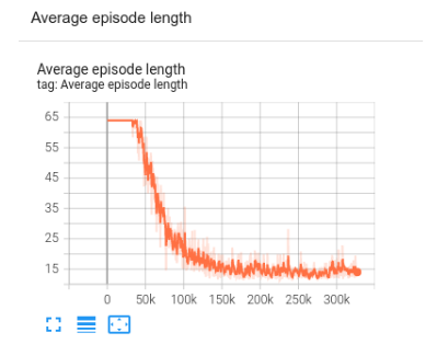
Since what we are doing isn’t supervised learning, we can’t really use training loss to monitor the training progress. Instead, we are going to use a proxy metric ‘game_length’, which indicates how many steps the agent takes to finish each episode. Intuitively you can understand that if the agent is smarter and makes better predictions, the game length becomes shorter.

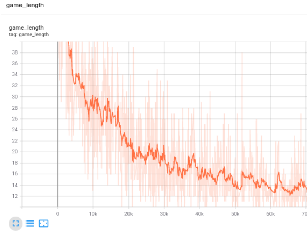
Training progress in TensorBoard

Since this is a game that needs instantaneous responses from the agent, we want to deploy the model on mobile devices instead of servers. After training the model, we use the TFLite converter to convert the Keras model into a TFLite model, and integrate it into our Android app.

converter = tf.lite.TFLiteConverter.from_keras_model(model)
tflite_model = converter.convert()

The exported model is very fast and takes <1 ms to execute on Pixel phones. During the game play, at each step the agent looks at the user’s board position and predicts its next strike position to achieve 8 red cells as fast as possible.

convertBoardStateToByteBuffer(board);
tflite.run(boardData, outputProbArrays);
float[] probArray = outputProbArrays[0];
int agentStrikePosition = -1;
float maxProb = 0;
for (int i = 0; i int x = i / Constants.BOARD_SIZE;
int y = i % Constants.BOARD_SIZE;
if (board[x][y] == BoardCellStatus.UNTRIED && probArray[i] > maxProb) {
agentStrikePosition = i;
maxProb = probArray[i];
}
}

TensorFlow Lite with a model trained with TensorFlow Agents

While it’s a good exercise to write our agent from scratch using TensorFlow API, it’s better to leverage existing implementations of RL algorithms. TensorFlow Agents is a library for reinforcement learning in TensorFlow, and makes it easier to design, implement and test new RL algorithms by providing well tested modular components that can be modified and extended. TF Agents has implemented several state-of-the-art RL algorithms, including DQN, DDPG, REINFORCE, PPO, SAC and TD3. Trained policies by TF Agents can be converted to TFLite directly and deployed into mobile apps (note that this feature is only recently enabled so you will need the nightly builds of TensorFlow and TensorFlow Agents).

We use the TF Agents REINFORCE agent to train our agent. First, we need to define a TF Agents training environment as we did with the gym environment in the previous section. Then we can define an actor net as our policy network


actor_net = tfa.networks.Sequential([
tfa.keras_layers.InnerReshape([BOARD_SIZE, BOARD_SIZE], [BOARD_SIZE**2]),
tf.keras.layers.Dense(FC_LAYER_PARAMS, activation='relu'),
tf.keras.layers.Dense(BOARD_SIZE**2),
tf.keras.layers.Lambda(lambda t: tfp.distributions.Categorical(logits=t)),
], input_spec=train_py_env.observation_spec(
))

We are going to use the built-in REINFORCE agent that TF Agents has already implemented. The agent is built on top of the ‘actor_net’ defined above:

  tf_agent = reinforce_agent.ReinforceAgent(
train_env.time_step_spec(),
train_env.action_spec(),
actor_network=actor_net,
optimizer=optimizer,
normalize_returns=True,
train_step_counter=train_step_counter)

To train the agent, we need to collect some trajectories as experience. We define a function just for that using DeepMind Reverb and TF Agent PyDriver:

def collect_episode(environment, policy, num_episodes, replay_buffer_observer):
"""Collect game episode trajectories."""
initial_time_step = environment.reset()

driver = py_driver.PyDriver(
environment,
py_tf_eager_policy.PyTFEagerPolicy(policy, use_tf_function=True),
[replay_buffer_observer],
max_episodes=num_episodes)
initial_time_step = environment.reset()
driver.run(initial_time_step)

Now we are ready to train the model:

for i in range(iterations):
# Collect a few episodes using collect_policy and save to the replay buffer.
collect_episode(train_py_env, collect_policy,
COLLECT_EPISODES_PER_ITERATION, replay_buffer_observer)

# Use data from the buffer and update the agent's network.
iterator = iter(replay_buffer.as_dataset(sample_batch_size=1))
trajectories, _ = next(iterator)
tf_agent.train(experience=trajectories)
replay_buffer.clear()

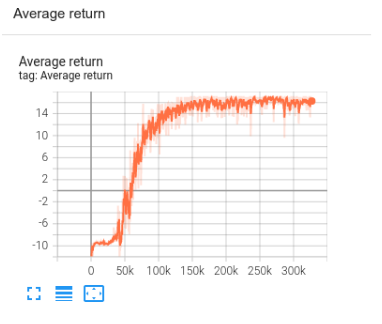
You can monitor the training progress using TensorBoard. In this case, we visualize both the average episode length and average return.

TF Agents training progress in TensorBoard

Once the policy has been trained and exported as SavedModel, you can converted it into a TFLite model:

converter = tf.lite.TFLiteConverter.from_saved_model(
policy_dir, signature_keys=['action'])
converter.target_spec.supported_ops = [
tf.lite.OpsSet.TFLITE_BUILTINS, # enable TensorFlow Lite ops.
tf.lite.OpsSet.SELECT_TF_OPS # enable TensorFlow ops.
]
tflite_policy = converter.convert()
with open(os.path.join(model_dir, 'planestrike_tf_agents.tflite'), 'wb') as f:
f.write(tflite_policy)

Currently there are a few TensorFlow ops that are required during the conversion. The converted model is slightly different from the model we trained using TensorFlow directly, because it takes 4 tensors as the input. What really matters here is the ‘observation’ tensor. Our agent will look at this ‘observation’ tensor and predict its next move. The other 3 can be safely ignored at inference time.

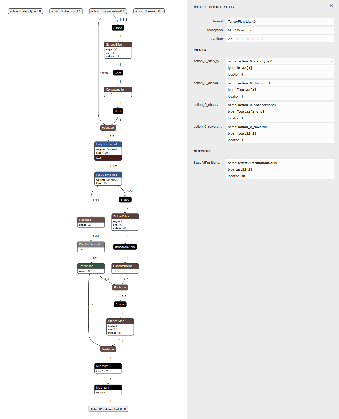
Visualizing TFLite model converted from TF Agents using Netron

Also, the model directly outputs the strike position instead of the probability distribution, so we no longer need to do argmax manually.

@Override
protected void runInference() {
Map output = new HashMap();
// TF Agent directly returns the predicted action
int[][] prediction = new int[1][1];
output.put(0, prediction);
tflite.runForMultipleInputsOutputs(inputs, output);
agentStrikePosition = prediction[0][0];

So to summarize, in this post we showed you 2 paths of how to train a game agent, convert the trained model to TFLite and deploy it into an Android app. Hopefully this end-to-end tutorial helps you better understand how to leverage the TensorFlow ecosystem to build cool games.

And lastly, if this little game looks interesting to you, we challenge you to install the app on your phone and see if you can beat the agent we have trained 😃.

Read More

TF Challenge Winners! Graphic

Announcing the Winners of the TensorFlow Lite for Microcontrollers Challenge!

Posted by Pete Warden for the TensorFlow team

TF Challenge Winners! Graphic

In May 2021, we published the TensorFlow Microcontroller Challenge, inviting developers to push the boundaries of TensorFlow Lite for Microcontrollers. Our sincere thanks go out to all those who participated in our competition and contributed to its success! Submissions came from 20 countries across 6 continents.

We’re excited to announce the five winning entries.

  • Mapping Dance by Eduardo Padrón: Take control of lighting and video projections with your dance moves.
  • Move! by Yongjae Kim, Jonghyun Baek, Eunji Lee, Yeonhee Kim, and Jueun Choi: Stay active, using movement to control a variety of games.
  • Snoring Guardian by Naveen Kumar: A snore-no-more device embedded in your pillow.
  • Squat Counter by Manas Pange: Focus on your form, while this tracker counts your squats.
  • Voice Turn by Alvaro Gonzalez-Vila: A safer way for cyclists to signal using their voice.

These projects push boundaries, spark joy, and show off the helpfulness of TensorFlow Lite for Microcontrollers. The teams who created them will each receive a prize and meet with the TensorFlow team.

To view the winning entries, check out the TensorFlow Lite for Microcontrollers collection on Experiments with Google. Read More

ML Community Day: Save the date

Posted by the TensorFlow team

Please join us for ML Community Day, a virtual developer event on November 9th. You’ll hear from the TensorFlow, JAX, and Deepmind teams and the community, covering new products, updates, and more.

This event takes place on TensorFlow’s sixth birthday (time flies!), and celebrates many years of open-source work by the developer community. We’ll have talks on on-device Machine Learning, JAX, Responsible AI, Cloud TPUs, Machine Learning in production, and sessions from the community.

You’ll also learn how you can get involved with the machine learning community by connecting with Google Developer Experts, joining Special Interest Groups, TensorFlow User Groups, and more.

Later in the day we’ll host the TensorFlow Contributor Summit, in which Google Developer Experts, Special Interest Groups, TensorFlow User Group organizers, and other community leaders gather to connect in a small group to discuss topics such as documentation and how to contribute to the TensorFlow ecosystem. During this event, we will also host the first TensorFlow Awards Ceremony to recognize outstanding community contributions.

You can find more details at the event website. We’ll see you soon!

Read More

Get Started with TensorFlow Lite Micro on Sony’s Spresense

A guest post by Daniel Sandblom, Sony

Editor’s note: an earlier version of this article appeared on the Sony Developers.

 Photo of a Sony Spresense microcontroller board

Now you can develop solutions with TensorFlow Lite Micro (TFLM) for the Spresense microcontroller board from Sony. TFLM is designed to run on microcontroller systems where the hardware resources are more limited compared to larger computerized systems. The footprint of TFLM is typically in the order of only 10’s of kBs.

What you get is a combination of a leading machine learning ecosystem with a high performance microcontroller running at super low power consumption. The Spresense board was designed with camera and hi-res audio inputs as core features which open up a substantial set of use cases. Pete Warden, a research engineer on the TensorFlow team, shares his view on that TFLM is now available for use with the Spresense board: “It’s great to see this kind of compute capability tightly integrated into a low power sensor, the combination will help make machine learning accessible to developers in medical, agriculture, industrial monitoring and many other areas where a small form factor and energy are strong constraints.”

The development of TFLM has been a tight collaboration between Google and Arm to optimize functionality while keeping the footprint to a minimum. Fredrik Knutsson, Team Lead at Arm, explains how TFLM has been optimized for the ARM processor architecture: “Arm’s open source CMSIS-NN library provides high performance implementations of common neural network functions for Arm Cortex-M processors. Arm’s engineers have worked closely with the TensorFlow team to develop optimized versions of the TensorFlow Lite kernels in the CMSIS-NN library, delivering extremely fast performance on Arm Cortex-M cores like Spresense.

How to get started with TensorFlow on Spresense

The easiest and quickest way to get started with TensorFlow on Spresense is to run one of the examples. There is one hello_world example that shows the basic steps and functionality. There is also a micro_speech example using Spresense’s audio abilities, and there’s a person_detection example utilizing the Spresense camera. The latter two examples demonstrate how to link visual and audio sensors to the inputs of TensorFlow models.

Below are the general steps to run the examples:

  1. Set up the Spresense SDK: Getting started with TensorFlow for Spresense
  2. Download the Spresense repository including the examples
  3. Build and Flash the binary into Spresense main board
  4. Run the example

Heads-up: we will run an upcoming webinar for “TensorFlow on Spresense” on October 14 – register here!

Check out these links for more info:

Read More

How DermAssist uses TensorFlow.js for on-device image quality checks

Posted by Miles Hutson and Aaron Loh, Google Health

At Google I/O in May, we previewed our DermAssist web application designed to help people understand issues related to their skin. The tool is designed to be easy to use. Upon opening it, users are expected to take three images of their skin, hair, or nail concern from multiple angles, and provide some additional information about themselves and their condition.

This product has been CE marked as a Class I medical device in the EU. It is not available in the United States.

We recognize that when users take pictures on their phone, some images could be blurry or have poor lighting. To address this, we initially added a “quality check” after images had been uploaded, which would prompt people to retake an image when necessary. However, these prompts could be a frustrating experience for them, depending on their upload speed, how long they took to acquire the image, and the multiple retakes it might require to pass the quality check.

Letting the user know they uploaded an image with insufficient quality and advising them to retake it before they proceed.

To improve their experience, we decided to give users image quality feedback both on-device as they line up a photo, and when they review the photo before uploading. The way this feature works can be seen below. As the user lines up their camera for a shot, they may get a notification that their environment has a lighting issue (right image). Or, they may be notified that they took a blurry photo as they moved their camera (left image); the model helpfully lets them know their image is blurred before they go to the trouble of uploading it. They can decide to go back and correct the issue without the need to upload the image.

Examples of poor lighting or blurry images that obtain real time feedback so the user knows to take a new photo

Developing the Model

When developing the model, it was important to ensure that the model could comfortably run on-device. One such architecture designed for that purpose is MobileNetV2, which we selected as the backbone for the model.

Our discussions with dermatologists highlighted recurrent issues with image quality, such as the image being too blurry, too badly lit, or inappropriate for interpreting skin diseases. We curated several datasets to tackle those issues, which also informed the outputs of the model. The datasets included a crowdsourced data collection, public datasets, data obtained from tele-dermatology services, and synthetically generated images, many of which were further labeled by trained human graders. Combined, we trained the model on more than 30k images.

We trained the model with multiple binary heads, one for each quality issue. In the diagram below, we see how the input image is fed into a MobileNet feature extractor. This feature embedding is then fed to multiple distinct fully connected layers, producing a binary output (yes/no), each corresponding to a certain quality issue.

The infrastructure we used to train the model was built using TensorFlow, and exported models in the standard SavedModel format.

Translating the model to TensorFlow.js

Our team’s infrastructure for training models makes use of TensorFlow examples, which meant that the exported SavedModel had nodes for loading and preprocessing TensorFlow Examples.

TensorFlow.js at present does not support such preprocessing nodes. Therefore, we modified the signature of the SavedModel to use the image input node after the preprocessing nodes as input to the model. We re-implemented the processing in our Angular integration below.

Having rebuilt the SavedModel in the correct format for conversion, we employed the TensorFlow.js converter to convert it to the TensorFlow.js model format, which consists of a JSON file identifying the model topology, as well as the weights in sharded bin files.

tensorflowjs_converter --input_format=keras /path/to/tfjs/signature/ /path/to/write/tfjs_model

Integrating TensorFlow.js with Observables and the Image Capture API

With the model trained, serialized, and made available for TensorFlow.js, it might feel like the job is pretty much done. However, we still had to integrate the TensorFlow.js model into our Angular 2 web application. While doing that, we had the goal that the model would ultimately be exposed as an API similar to other components. A good abstraction would allow frontend engineers to work with the TensorFlow.js model as they would work with any other part of the application, rather than as a unique component.

To begin, we created a wrapper class around the model ImageQualityPredictor. This Typescript class exposed only two methods:

  1. A static method createImageQualityPredictor that, given a URL for the model, returns a promise for an ImageQualityPredictor.
  2. A makePrediction method that takes ImageData and returns an array of quality predictions above a given threshold.

We found that the implementation of makePrediction was key for abstracting the inner workings of our model. The result of calling execute on our model was an array of Tensors representing yes/no probabilities for each binary head. But we didn’t want the downstream application code to be responsible for the delicate task of thresholding these tensors and connecting them back to the heads’ descriptions. Instead, we moved these details inside of our wrapper class. The final return value to the caller was instead an interface ImageQualityPrediction.

export interface ImageQualityPrediction {
score: number;
qualityIssue: QualityIssue;
}

In order to make sure that a single ImageQualityPredictor was shared across the application, we in turn wrapped ImageQualityPredictor in a singleton ImageQualityModelService. This service handled the initialization of the predictor and tracked if the predictor already had a request in progress. It also contained helper methods for extracting frames from the ImageCapture API that our camera feature is built on and translating QualityIssue to plain English strings.

Finally, we combined the CameraService and our ImageQualityModelService in an ImageQualityService. The final product exposed for use in any given front end component is a simple observable that provides text describing any quality issues.

@Injectable()
export class ImageQualityService {
readonly realTimeImageQualityText$: Observable;

constructor(
private readonly cameraService: CameraService,
private readonly imageQualityModelService: ImageQualityModelService) {
const retrieveText = () =>
this.imageQualityModelService.runModel(this.cameraService.grabFrame());
this.realTimeImageQualityText$ =
interval(REFRESH_INTERVAL_MS)
.pipe(
filter(() => !imageQualityModelService.requestInProgress),
mergeMap(retrieveText),
);
}
// ...
}

This lends itself well to Angular’s normal templating system, accomplishing our goal of making a TensorFlow.js model in Angular as easy to work with as any other component for front end engineers. For example, a suggestion chip can be as easy to include in a component as

 <suggestive-chip *ngIf="(imageQualityText$ | async) as text"
>{{text}}</suggestive-chip>

Looking Ahead

With helping users to capture better pictures in mind, we developed an on-device image quality check for the DermAssist app to provide real-time guidance on image intake. Part of making users’ lives easier is making sure that this model works fast enough such that we can show a notification as quickly as possible while they’re taking a picture. For us, this means finding ways to reduce the model size in order to reduce the time it takes to load on a user’s device. Possible techniques to further advance this goal may be model quantization, or attempts at model distillation into smaller architectures.

To learn more about the DermAssist application, check out our blog post from Google I/O.

To learn more about TensorFlow.js, you can visit the main site here, also be sure to check out the tutorials and guide.

Read More

TensorFlow Model Optimization Toolkit — Collaborative Optimization API

A guest post by Mohamed Nour Abouelseoud and Elena Zhelezina at Arm.

This blog post introduces collaborative techniques for machine learning model optimization for edge devices, proposed and contributed by Arm to the TensorFlow Model Optimization Toolkit, available starting from release v0.7.0.

The main idea of the collaborative optimization pipeline is to apply the different optimization techniques in the TensorFlow Model Optimization Toolkit one after another while maintaining the balance between compression and accuracy required for deployment. This leads to significant reduction in the model size and could improve inference speed given framework and hardware-specific support such as that offered by the Arm Ethos-N and Ethos-U NPUs.

This work is a part of the toolkit’s roadmap to support the development of smaller and faster ML models. You can see previous posts on post-training quantization, quantization-aware training, sparsity, and clustering for more background on the toolkit and what it can do.

What is Collaborative Optimization? And why?

The motivation behind collaborative optimization remains the same as that behind the Model Optimization Toolkit (TFMOT) in general, which is to enable model conditioning and compression for improving deployment to edge devices. The push towards edge computing and endpoint-oriented AI creates high demand for such tools and techniques. The Collaborative Optimization API stacks all of the available techniques for model optimization to take advantage of their cumulative effect and achieve the best model compression while maintaining required accuracy.

Given the following optimization techniques, various combinations for deployment are possible:

In other words, it is possible to apply one or both of pruning and clustering, followed by post-training quantization or QAT before deployment.

The challenge in combining these techniques is that the APIs don’t consider previous ones, with each optimization and fine-tuning process not preserving the results of the preceding technique. This spoils the overall benefit of simultaneously applying them; i.e., clustering doesn’t preserve the sparsity introduced by the pruning process and the fine-tuning process of QAT loses both the pruning and clustering benefits. To overcome these problems, we introduce the following collaborative optimization techniques:

Considered together, along with the option of post-training quantization instead of QAT, these provide several paths for deployment, visualized in the following deployment tree, where the leaf nodes are deployment-ready models, meaning they are fully quantized and in TFLite format. The green fill indicates steps where retraining/fine-tuning is required and a dashed red border highlights the collaborative optimization steps. The technique used to obtain a model at a given node is indicated in the corresponding label.

Keras Model Flow Chart

The direct, quantization-only (post-training or QAT) deployment path is omitted in the figure above.

The idea is to reach the fully optimized model at the third level of the above deployment tree; however, any of the other levels of optimization could prove satisfactory and achieve the required inference latency, compression, and accuracy target, in which case no further optimization is needed. The recommended training process would be to iteratively go through the levels of the deployment tree applicable to the target deployment scenario and see if the model fulfils the optimization requirements and, if not, use the corresponding collaborative optimization technique to compress the model further and repeat until the model is fully optimized (pruned, clustered, and quantized), if needed.

To further unlock the improvements in memory usage and speed at inference time associated with collaborative optimization, specialized run-time or compiler software and dedicated machine learning hardware is required. Examples include the Arm ML Ethos-N driver stack for the Ethos-N processor and the Ethos-U Vela compiler for the Ethos-U processor. Both examples currently require quantizing and converting optimized Keras models to TensorFlow Lite first.

The figure below shows the density plots of a sample weight kernel going through the full collaborative optimization pipeline.

Quantized deployment model with reduced number of unique values

The result is a quantized deployment model with a reduced number of unique values as well as a significant number of sparse weights, depending on the target sparsity specified at training time. This results in substantial model compression advantages and significantly reduced inference latency on specialized hardware.

Compression and accuracy results

The tables below show the results of running several experiments on popular models, demonstrating the compression benefits vs. accuracy loss incurred by applying these techniques. More aggressive optimizations can be applied, but at the cost of accuracy. Though the table below includes measurements for TensorFlow Lite models, similar benefits are observed for other serialization formats.

Sparsity-preserving Quantization aware training (PQAT)

Model

Metric

Baseline

Pruned Model (50% sparsity)

QAT Model

PQAT Model

DS-CNN-L

FP32 Top-1 Accuracy

95.23%

94.80%

(Fake INT8) 94.721%

(Fake INT8) 94.128%

INT8 Top-1 Accuracy

94.48%

93.80%

94.72%

94.13%

Compression

528,128 → 434,879 (17.66%)

528,128 → 334,154 (36.73%)

512,224 → 403,261 (21.27%)

512,032 → 303,997 (40.63%)

MobileNet_v1 on ImageNet

FP32 Top-1 Accuracy

70.99%

70.11%

(Fake INT8) 70.67%

(Fake INT8) 70.29%

INT8 Top-1 Accuracy

69.37%    

67.82%

70.67%    

70.29%

Compression

4,665,520 → 3,880,331 (16.83%)

4,665,520 → 2,939,734 (37.00%)

4,569,416 → 3,808,781 (16.65%)

4,569,416 → 2,869,600 (37.20%)

Note: DS-CNN-L is a keyword spotting model designed for edge devices. More can be found in Arm’s ML Examples repository.

Cluster-preserving Quantization aware training (CQAT)

Model

Metric

Baseline

Clustered Model

QAT Model

CQAT Model

MobileNet_v1 on CIFAR-10

FP32 Top-1 Accuracy

94.88%

94.48% (16 clusters)    

(Fake INT8) 94.80%

(Fake INT8) 94.60%

INT8 Top-1 Accuracy

94.65%    

94.41% (16 clusters)    

94.77%

94.52%

Size

3,000,000

2,000,000

2,840,000

1,940,000

MobileNet_v1 on ImageNet

FP32 Top-1 Accuracy

71.07%

65.30% (32 clusters)

(Fake INT8) 70.39%

(Fake INT8) 65.35%

INT8 Top-1 Accuracy

69.34%    

60.60% (32 clusters)

70.35%

65.42%

Compression

4,665,568 → 3,886,277 (16.7%)

4,665,568 → 3,035,752 (34.9%)

4,569,416 → 3,804,871 (16.7%)

4,569,472 → 2,912,655 (36.25%)

Sparsity and cluster preserving quantization aware training (PCQAT)

Model

Metric

Baseline

Pruned Model (50% sparsity)

QAT Model

Pruned Clustered Model

PCQAT Model

DS-CNN-L

FP32 Top-1 Accuracy

95.06%

94.07%    

(Fake INT8) 94.85%

93.76% (8 clusters)    

(Fake INT8) 94.28%

INT8 Top-1 Accuracy

94.35%    

93.80%    

94.82%    

93.21% (8 clusters)

94.06%

Compression

506,400 → 425,006 (16.07%)

506,400 → 317,937 (37.22%)

507,296 → 424,368 (16.35%)

506,400 → 205,333

(59.45%)

507,296 → 201,744 (60.23%)

MobileNet_v1 on ImageNet

FP32 Top-1 Accuracy

70.98%

70.49%

(Fake INT8) 70.88%

67.64% (16 clusters)

(Fake INT8) 67.80%

INT8 Top-1 Accuracy

70.37%

69.85%    

70.87%    

66.89% (16 clusters)    

68.63%

Compression

4,665,552 →  3,886,236 (16.70%)

4,665,552 →  2,909,148 (37.65%)

4,569,416 → 3,808,781 (16.65%)

4,665,552 →  2,013,010 (56.85%)    

4,569472 →  1,943,957 (57.46%)

Applying PCQAT

To apply PCQAT, you will need to first use the pruning API to prune the model, then chain it with clustering using the sparsity-preserving clustering API. After that, the QAT API is used along with the custom collaborative optimization quantization scheme. An example is shown below.

import tensorflow_model_optimization as tfmot
model = build_your_model()

# prune model
model_for_pruning = tfmot.sparsity.keras.prune_low_magnitude(model, ...)

model_for_pruning.fit(...)

# pruning wrappers must be stripped before clustering
stripped_pruned_model = tfmot.sparsity.keras.strip_pruning(pruned_model)

After pruning the model, cluster and fit as below.

# Sparsity preserving clustering
from tensorflow_model_optimization.python.core.clustering.keras.experimental import (cluster)

# Specify your clustering parameters along
# with the `preserve_sparsity` flag
clustering_params = {
...,
'preserve_sparsity': True
}

# Cluster and fine-tune as usual
cluster_weights = cluster.cluster_weights
sparsity_clustered_model = cluster_weights(stripped_pruned_model_copy, **clustering_params)
sparsity_clustered_model.compile(...)
sparsity_clustered_model.fit(...)

# Strip clustering wrappers before the PCQAT step
stripped_sparsity_clustered_model = tfmot.clustering.keras.strip_clustering(sparsity_clustered_model)

Then apply PCQAT.

pcqat_annotate_model = quantize.quantize_annotate_model(stripped_sparsity_clustered_model )
pcqat_model = quantize.quantize_apply(quant_aware_annotate_model,scheme=default_8bit_cluster_preserve_quantize_scheme.Default8BitClusterPreserveQuantizeScheme(preserve_sparsity=True))
pcqat_model.compile(...)
pcqat_model.fit(...)

The example above shows the training process to achieve a fully optimized PCQAT model, for the other techniques, please refer to the CQAT, PQAT, and sparsity-preserving clustering example notebooks. Note that the API used for PCQAT is the same as that of CQAT, the only difference being the use of the preserve_sparsity flag to ensure that the zero cluster is preserved during training. The PQAT API usage is similar but uses a different, sparsity preserving, quantization scheme.

Acknowledgments

The features and results presented in this post are the work of many people including the Arm ML Tooling team and our collaborators in Google’s TensorFlow Model Optimization Toolkit team.

From Arm – Anton Kachatkou, Aron Virginas-Tar, Ruomei Yan, Saoirse Stewart, Peng Sun, Elena Zhelezina, Gergely Nagy, Les Bell, Matteo Martincigh, Benjamin Klimczak, Thibaut Goetghebuer-Planchon, Tamás Nyíri, Johan Gras.

From Google – David Rim, Frederic Rechtenstein, Alan Chiao, Pulkit Bhuwalka

Read More

End-to-end tinyML audio classification with the Raspberry Pi RP2040

A guest post by Sandeep Mistry, Arm

Image of tools you’ll need for the project
Some tools you’ll need for this project (learn more below!)

Introduction

Machine learning enables developers and engineers to unlock new capabilities in their applications. Instead of explicitly defining instructions and rules for a computer to execute, you can collect large amounts of data for a classification task that your application requires, and train an ML model to learn from the patterns in the data.

Training typically happens in the cloud on computers equipped with one or more GPUs. Once a model has been trained, depending on its size, it can be deployed for inference on a wide range of devices. These devices range from large computers in the cloud with gigabytes of memory, to tiny microcontrollers (or MCUs) which typically have just kilobytes of memory.

Microcontrollers are low-power, self-contained, cost-effective computer systems that are embedded in devices that you use everyday, such as your microwave, electric toothbrush, or smart door lock. Microcontroller based systems typically interact with their surrounding environment via one or more sensors (think buttons, microphones, motion sensors) and perform an action using one or more actuators (think LEDs, motors, speakers).

Microcontrollers also offer privacy advantages, and can perform inference locally on the device, without needing to send any data to the cloud. This can have power advantages too for devices running off batteries.

In this article, we will demonstrate how an Arm Cortex-M based microcontroller can be used for local on-device ML to detect audio events from its surrounding environment. This is a tutorial-style article, and we’ll guide you through training a TensorFlow based audio classification model to detect a fire alarm sound.

We’ll show you how to use TensorFlow Lite for Microcontrollers with Arm CMSIS-NN accelerated kernels to deploy the ML model to an Arm Cortex-M0+ based microcontroller board for local on-device ML inference. Arm’s CMSIS-DSP library, which provides optimized Digital Signal Processing (DSP) function implementations for Arm Cortex-M processors, will also be used to extract features from the real-time audio data before inference.

While this guide focuses on detecting a fire alarm sound, it can be adapted for other sound classification tasks. You may also need to adapt the feature extraction stages and/or adjust ML model architecture for your use case.

An interactive version of this tutorial is available on Google Colab and all technical assets for this guide can be found on GitHub.

What you need to to get started

Development Environment

Hardware

You’ll need one of the following development boards that are based on Raspberry Pi’s RP2040 MCU chip that was released early in 2021.

SparkFun RP2040 MicroMod and MicroMod ML Carrier

This board is great for folks new to electronics and microcontrollers. It does not require a soldering iron, knowing how to solder, or how to wire up breadboards.

Image of tools you’ll need for the project

Raspberry Pi Pico and PDM microphone board

This option is great if you know how to solder (or would like to learn). It requires a soldering iron and knowledge of how to wire a breadboard with electronic components. You’ll need:

Image of Raspberry Pi Pico and PDM microphone board

Both of the options above will allow you to collect real-time 16 kHz audio from a digital microphone and process the audio signal on the development board’s Arm Cortex-M0+ processor, which operates at 125 MHz. The application running on the Arm Cortex-M0+ will have a Digital Signal Processing (DSP) stage to extract features from the audio signal. The extracted features will then be fed into a neural network to perform a classification task to determine if a fire alarm sound is present in the board’s environment.

Dataset

We will start by training a sound classifier (for many events) with TensorFlow using the ESC-50: Dataset for Environmental Sound Classification. After training on this broad dataset, we will use Transfer Learning to fine tune it for our specific audio classification task.

This model will be trained on the ESC-50 dataset, which contains 50 types of sounds. Each sound category has 40 audio files that are 5 seconds each in length. Each audio file will be split into 1 second soundbites, and any soundbites that contain pure silence will be discarded.

Image shows a sample waveform from the data set of a dog barking
A sample waveform from the data set of a dog barking.

Spectrograms

Rather than passing in the time series data directly into our TensorFlow model, we will transform the audio data into an audio spectrogram representation. This will create a 2D representation of the audio signal’s frequency content over time.

The input audio signal we will use will have a sampling rate of 16kHz, this means one second of audio will contain 16,000 samples. Using TensorFlow’s tf.signal.stft(…) function we can transform a 1 second audio signal into a 2D tensor representation. We will choose a frame length of 256 and a frame step of 128, so the output of this feature extraction stage will be a Tensor that has a shape of (124, 129).

Image shows An audio spectrogram representation of a dog barking.
An audio spectrogram representation of a dog barking.

The ML model

Now that we have the features extracted from the audio signal, we can create a model using TensorFlow’s Keras API. You can find the complete code linked above. The model will consist of 8 layers:

  1. An input layer.
  2. A preprocessing layer, that will resize the input tensor from 124x129x1 to 32x32x1.
  3. A normalization layer, that will scale the input values between -1 and 1
  4. A 2D convolution layer with: 8 filters, a kernel size of 8×8, and stride of 2×2, and ReLU activation function.
  5. A 2D max pooling layer with size of 2×2
  6. A flatten layer to flatten the 2D data to 1D
  7. A dropout layer, that will help reduce overfitting during training
  8. A dense layer with 50 outputs and a softmax activation function, which outputs the likelihood of the sound category (between 0 and 1).

The model summary can be found below:

Image of model summary

Notice that this model only has about 15K parameters (this is quite small!)

Fine tuning

Now we will use transfer learning and change the classification head (the last Dense layer) of the model to train a binary classification model for fire alarm sounds. We have collected 10 fire alarm clips from freesound.org and BigSoundBank.com. Background noise clips from the SpeechCommands dataset will be used for non-fire alarm sounds. This dataset is small, and enough for us to get started. Data augmentation techniques will be used to supplement the training data we’ve collected.

For real-world applications, it’s important to collect a much larger dataset (you can learn more about best practices on TensorFlow’s Responsible AI website).

Data Augmentation

Data augmentation is a set of techniques used to increase the size of a dataset. This is done by slightly modifying samples from the dataset or by creating synthetic data. In this situation we are using audio and we will create a few functions to augment different samples. We will use three techniques:

  1. Adding white noise to the audio samples.
  2. Adding random silence to the audio.
  3. Mixing two audio samples together.

As well as increasing the size of the dataset, data augmentation also helps to reduce overfitting by training the model on different (not perfect) data samples. For example, on a microcontroller you are unlikely to have perfect high quality audio, and so a technique like adding white noise can help the model work in situations where your microphone might every so often have noise in there.

A gif showing how data augmentation slightly changes the spectrogram by adding noise
A gif showing how data augmentation slightly changes the spectrogram by adding noise (watch it closely, it can be a bit hard to see).

Feature Extraction

TensorFlow Lite for Microcontroller (TFLu) provides a subset of TensorFlow operations, so we are unable to use the tf.signal.sft(…) API we’ve used for feature extraction of the baseline model on our MCU. However, we can leverage Arm’s CMSIS-DSP library to generate spectrograms on the MCU. CMSIS-DSP contains support for both floating-point and fixed-point DSP operations which are optimized for Arm Cortex-M processors, including the Arm Cortex-M0+ that we will be deploying the ML model to. The Arm Cortex-M0+ does not contain a floating-point unit (FPU) so it would be better to leverage a 16-bit fixed-point DSP based feature extraction pipeline on the board.

We can leverage CMSIS-DSP’s Python Wrapper in the notebook to perform the same operations on our training pipeline using 16-bit fixed-point math. At a high level we can replicate the TensorFlow SFT API with the following CMSIS-DSP based operations:

  1. Manually creating a Hanning Window of length 256 using the Hanning Window formula along with CMSIS-DSP’s arm_cos_f32 API.
    Screenshot showing the Hanning Window formula
  2. Creating a CMSIS-DSP arm_rfft_instance_q15 instance and initializing it using CMSIS-DSP’s arm_rfft_init_q15 API.
  3. Looping through the audio data 256 samples at a time, with a stride of 128 (this matches the parameters we’ve passed into the TF sft API)
    1. Multiplying the 256 samples by the Hanning Window, using CMSIS-DSP’s arm_mult_q15 API
    2. Calculating the FFT of the output of the previous step, using CMSIS-DSP’s arm_rfft_q15 API
    3. Calculating the magnitude of the previous step, using CMSIS-DSP’s arm_cmplx_mag_q15 API
  4. Each audio soundbites’s FFT magnitude represents the one column of the spectrogram.
  5. Since our baseline model expects a floating point input, instead of the 16-bit quantized value we were using, the CMSIS-DSP arm_q15_to_float API can be used to convert the spectrogram data from a 16-bit fixed-point value to a floating-point value for training.

The complete Python code for this is a bit long, but can be found in the “Transfer Learning -> Load dataset” section of the Google Colab notebook.

Image of waveform and audio spectrogram of a smoke alarm sound.
Waveform and audio spectrogram of a smoke alarm sound.

For an in-depth description of how to create audio spectrograms using fixed-point operations with CMSIS-DSP, please see Towards Data Science “Fixed-point DSP for Data Scientists” guide.

Loading the baseline model and changing the classification head

The model we previously trained on the ESC-50 dataset, predicted the presence of 50 sound types, and which resulted in the final dense layer of the model having 50 outputs. The new model we would like to create is a binary classifier, and needs to have a single output value.

We will load the baseline model, and swap out the final dense layer to match our needs:

# We need a new head with one neuron.
model_body = tf.keras.Model(inputs=model.input, outputs=model.layers[-2].output)

classifier_head = tf.keras.layers.Dense(1, activation="sigmoid")(model_body.output)

fine_tune_model = tf.keras.Model(model_body.input, classifier_head)

This results in the following model.summary():

Screenshot of model summary

Transfer Learning

Transfer Learning is the process of retraining a model that has been developed for a task to complete a new similar task. The idea is that the model has learned transferable “skills” and the weights and biases can be used in other models as a starting point.

As humans we use transfer learning too. The skills you developed to learn to walk could also be used to learn to run later on.

In a neural network, the first few layers of a model start to perform a “feature extraction” such as finding shapes, edges and colours. The layers later on are used as classifiers; they take the extracted features and classify them.

Because of this, we can assume the first few layers have learned quite general feature extraction techniques that can be applied to similar tasks, and so we can freeze all these layers and use them on a new task in the future. The classifier layer will need to be trained based on the new task.

To do this, we break the process into two steps:

  1. Freeze the “backbone” of the model and train the head with a fairly high learning rate. We slowly reduce the learning rate.
  2. Unfreeze the “backbone” and fine-tune the model with a low learning rate.

To freeze a layer in TensorFlow we can set layer.trainable=False. Let’s loop through all the layers and do this:

for layer in fine_tune_model.layers:
layer.trainable = False

and now unfreeze the last layer (the head):

fine_tune_model.layers[-1].trainable = True

We can now train the model using a binary crossentropy loss function. Keras callbacks for early stopping (to avoid overfitting) and a dynamic learning rate scheduler will also be used.

After we’ve trained with the frozen layers, we can unfreeze them:

for layer in fine_tune_model.layers:
layer.trainable = True

And train again for up to 10 epochs. You can find the complete code for this in the “Transfer Learning -> ”Train Model” section of Colab notebook.

Recording your own training data

We now have an ML model which can classify the presence of fire alarm sound. However this model was trained on publicly available sound recordings which might not match the sound characteristics of the hardware microphone we will use for inferencing.

The Raspberry Pi RP2040 MCU has a native USB feature that allows it to act like a custom USB device. We can flash an application to the board to enable it to act like a USB microphone to our PC. Then we can extend Google Colab’s capabilities with the Web Audio API on a modern Web browser like Google Chrome to collect live data samples (all from within Google Colab!)

Hardware Setup

SparkFun MicroMod RP2040

For assembly, remove the screw on the carrier board, at an angle, slide in the MicroMod RP2040 Processor board into the socket and secure it in place with the screw. See the MicroMod Machine Learning Carrier Board Hookup Guide for more details.

Image of removing the screw on the carrier board

Raspberry Pi Pico

Follow the instructions from the Hardware Setup section of the “Create a USB Microphone with the Raspberry Pi Pico” guide for assembly instructions.

Top: Fritzing wiring diagram Bottom: Assembled breadboard

Setting up the firmware applications toolchains

Rather than setting up the Raspberry Pi Pico’s SDK on your personal computer. We can leverage Colab’s built-in Linux shell command feature to set up the Pico SDK development environment with CMake and GNU Arm Embedded Toolchain.

The pico-sdk will also have to be downloaded to the Colab instance using git:

%%shell
git clone https://github.com/raspberrypi/pico-sdk.git
cd pico-sdk
git submodule init
git submodule update

Compiling and flashing the USB microphone application

Now we can use the USB microphone example from the Microphone Library for Pico. The example application can be compiled using cmake and make. Then we can flash the example application to the board over USB by putting the board into “boot ROM mode” which will allow us to upload an application to the board.

SparkFun

  • Plug the USB-C cable into the board and your PC to power the board.
  • While holding down the BOOT button on the board, tap the RESET button.

GIF shows holding down the BOOT button on the board, and tapping the RESET button

Raspberry Pi Pico

  • Plug the USB Micro cable into your PC, but do NOT plug in the Pico side.
  • While holding down the white BOOTSEL button, plug in the micro USB cable to the Pico.

GIF shows plugging in the micro USB cable to the Pico

If you are using a WebUSB API enabled browser like Google Chrome, you can directly flash the image onto the board from within Google Collab!

GIF showing Downloading USB microphone application to the board from within Google Colab and WebUSB

Downloading USB microphone application to the board from within Google Colab and WebUSB.

Otherwise, you can manually download the .uf2 file to your computer and then drag it onto the USB disk for the RP2040 board.

Collecting training data

Now that you have flashed the USB microphone application to the board, it will appear as a USB audio input on your PC.

We can now use Google Colab to record a fire alarm sound, select “MicNode ” as the audio input source in the drop down. Then while pressing the test button on a smoke alarm, click the record button on Google Colab to record a 1 second audio clip. Repeat this process a few times.

Similarly, we can also do the same to collect background audio samples in the next code cell in Google Colab. Repeat this a few times for non-fire alarm sounds like silence, yourself talking, or any other normal sounds for the environment.

Final model training

Now that we’ve collected additional samples with the microphone that will be used during inference. We can tune the model again with the new data.

Converting the Model to run on the MCU

We will need to convert the Keras model we’ve used to TensorFlow Lite format so that we can use it for inference on the device.

Quantization

To optimize the model to run on the Arm Cortex-M0+ processor, we will use a process called model quantization. Model quantization converts the model’s weights and bias from 32-bit floating point values to 8-bit values. The pico-tflmicro library, which is a port of TFLu for the RP2040’s Pico SDK contains Arm’s CMSIS-NN library, which supports optimized kernel operations for quantized 8-bit weights on Arm Cortex-M processors.

We can use TensorFlow’s Quantization Aware Training (QAT) feature to easily convert the floating-point model to quantized.

Converting the model to TF Lite format

We will now use the tf.lite.TFLiteConverter.from_keras_model(…) API to convert the quantized Keras model to TF Lite format, and then save it to disk as a .tflite file.

converter = tf.lite.TFLiteConverter.from_keras_model(quant_aware_model)
converter.optimizations = [tf.lite.Optimize.DEFAULT]

train_ds = train_ds.unbatch()

def representative_data_gen():
for input_value, output_value in train_ds.batch(1).take(100):
# Model has only one input so each data point has one element.
yield [input_value]

converter.representative_dataset = representative_data_gen
# Ensure that if any ops can't be quantized, the converter throws an error
converter.target_spec.supported_ops = [tf.lite.OpsSet.TFLITE_BUILTINS_INT8]
# Set the input and output tensors to uint8 (APIs added in r2.3)
converter.inference_input_type = tf.int8
converter.inference_output_type = tf.int8
tflite_model_quant = converter.convert()

with open("tflite_model.tflite", "wb") as f:
f.write(tflite_model_quant)

Since TensorFlow also supports loading TF Lite models using tf.lite, we can also verify the functionality of the quantized model and compare its accuracy with the regular unquantized model inside Google Colab.

The RP2040 MCU on the boards we are deploying to, does not have a built-in file system, which means we cannot use the .tflite file directly on the board. However, we can use the Linux `xxd` command to convert the .tflite file to a .h file which can then be compiled in the inference application in the next step.

%%shell
echo "alignas(8) const unsigned char tflite_model[] = {" > tflite_model.h
cat tflite_model.tflite | xxd -i >> tflite_model.h
echo "};"

Deploy the model to the device

We now have a model that is ready to be deployed to the device. We’ve created an application template for inference which can be compiled with the .h file that we’ve generated for the model.

The C++ application uses the pico-sdk as the base, along with the CMSIS-DSP, pico-tflmicro, and Microphone Library for Pico libraries. It’s general structure is as follows:

  1. Initialization
    1. Configure the board’s built-in LED for output. The application will map the brightness of the LED to the output of the model. (0.0 LED off, 1.0 LED on with full brightness)
    2. Setup the TF Lite library and TF Lite model for inference
    3. Setup the CMSIS-DSP based DSP pipeline
    4. Setup and start the microphone for real-time audio
  2. Inference loop
    1. Wait for 128 * 4 = 512 new audio samples from the microphone
    2. Shift the spectrogram array over by 4 columns
    3. Shift the audio input buffer over by 128 * 4 = 512 samples and copy in the new samples
    4. Calculate 4 new spectrogram columns for the updated input buffer
    5. Perform inference on the spectrogram data
    6. Map the inference output value to the on-board LED’s brightness and output the status to the USB port

In-order to run in real-time each cycle of the inference loop must take under (512 / 16000) = 0.032 seconds or 32 milliseconds. The model we’ve trained and converted takes 24 ms for inference, which gives us ~8 ms for the other operations in the loop.

128 was used above to match the stride of 128 used in the training pipeline for the spectrogram. We used a shift of 4 in the spectrogram to fit within the real-time constraints we had.

Compiling the Firmware

Now we can use CMake to generate the build files required for compilation followed by make to compile.

The “cmake ..” line will have to be changed based on the board you are using:

  • SparkFun: cmake .. -DPICO_BOARD=sparkfun_micromod
  • Raspberry Pi Pico: cmake .. -DPICO_BOARD=pico

Flashing the Inference Application to the board

You’ll need to put the board into “boot ROM mode” again to load the new application to it.

SparkFun

  • Plug the USB-C cable into the board and your PC to power the board.
  • While holding down the BOOT button on the board, tap the RESET button.

Raspberry Pi Pico

  • Plug the USB Micro cable into your PC, but do NOT plug in the Pico side.
  • While holding down the white BOOTSEL button, plug in the micro USB cable to the Pico.

If you are using a WebUSB API enabled browser like Google Chrome, you can directly flash the image onto the board from within Google Colab. Otherwise, you can manually download the .uf2 file to your computer and then drag it onto the USB disk for the RP2040 board.

Monitoring the Inference on the board

Now that the inference application is running on the board you can observe it in action in two ways:

Visually by observing the brightness of the LED on the board. It should remain off or dim when no fire alarm sound is present – and be on when a fire alarm sound is present:

GIF shows LED on the board flashing

Connecting to the board’s USB serial port to view output from the inference application. If you are using a Web Serial API enabled browser like Google Chrome, this can be done directly from Google Colab:

GIF shows connecting to the board’s USB serial port to view output from the inference application

Improving the model

You now have the first version of the model deployed to the board, and it is performing inference on live 16,000 kHz audio data!

Test out various sounds to see if the model has the expected output. Maybe the fire alarm sound is being falsely detected (false positive) or not detected when it should be (false negative).

If this occurs, you can record more new audio data for the scenario(s) by flashing the USB microphone application firmware to the board, recording the data for training, re-training the model and converting to TF lite format, and re-compiling + flashing the inference application to the board.

Supervised machine learning models can generally only be as good as the training data they are trained with, so additional training data for these scenarios might help. You can also try to experiment with changing the model architecture or feature extraction process – but keep in mind that your model must be small enough and fast enough to run on the RP2040 MCU.

Conclusion

This article covered an end-to-end flow of how to train a custom audio classifier model to run locally on a development board that uses an Arm Cortex-M0+ processor. TensorFlow was used to train the model using transfer learning techniques along with a smaller dataset and data augmentation techniques. We also collected our own data from the microphone that is used at inference time by loading an USB microphone application to the board, and extending Colab’s features with the Web Audio API and JavaScript.

The training side of the project combined Google’s Colab service and Chrome browser, with the open source TensorFlow library. The inference application captured audio data from a digital microphone, used Arm’s CMSIS-DSP library for the feature extraction stage, then used TensorFlow Lite for Microcontrollers with Arm CMSIS-NN accelerated kernels to perform inference with a 8-bit quantized model that classified a real-time 16 kHz audio input on an Arm Cortex-M0+ processor.

The Web Audio API, Web USB API, and Web Serial API features of Google Chrome were used to extend Google Colab’s functionality to interact with the development board. This allowed us to experiment with and develop our application entirely with a web browser and deploy it to a constrained development board for on-device inference.

Since the ML processing was performed on the development boards RP2040 MCU, no audio data left the device at inference time.

Learn more

You can learn more and get hands-on experience using TinyML at the upcoming Arm DevSummit, a 3-day virtual event between October 19 – 21. The event includes workshops on tinyML computer vision for real-world embedded devices and building large vocabulary voice control with Arm Cortex-M based MCUs. We hope to see you there!

Read More

Join us at the Women in Machine Learning Symposium

Posted by Jeanine Banks, VP of 3P Core Developer Platforms

Join us for the Women in Machine Learning Symposium on October 19

At Google we believe that diversity and inclusion are core to innovation, and we know there’s work to be done in improving representation to achieve equity. That’s why we’re excited to announce a new event: The Women in Machine Learning Symposium.

Join us virtually from 9-12 PDT on October 19, 2021, to hear from leaders in the machine learning (ML) industry.

All journeys are different and this event aims to empower the next generation of women leaders in ML. By learning from each other’s stories we want to inspire the creation of a community of support, bringing together women and allies in technology.

We’ll have two keynotes discussing the importance of diversity in ML communities and Open Source Software. You can also hear first-hand the stories and experiences of women who are breaking down barriers and ask them questions live!

Lastly, I invite you to attend one of the breakout sessions tailored to what stage you’re at in your career. From learning how to get started in ML, how to switch from being a tech developer to becoming an ML developer, to learning tips for taking your career to the C-level, this event has a place for you.

RSVP today to reserve your spot and head on over to our website to view the live agenda. I hope to see you there!

Read More

Optical character recognition with TensorFlow Lite: A new example app

Posted by Wei Wei, TensorFlow Developer Advocate

As the old adage goes, “a picture is worth a thousand words.” Images are rich in visual information, but sometimes the key is with the text within. While it is easy for literate human beings to read words embedded in images, how do we use computer vision and machine learning to teach computers to do so?

Today, we are going to show you how to use TensorFlow Lite to extract text from images on Android devices. We will walk you through the key steps of the Optical Character Recognition (OCR) Android app that we recently open sourced here, which you can refer to for the complete code. You can see how the app extracts the product names from three Google product logos in the animation below.

Optical Character Recognition demo

The process of recognizing text from images is called Optical Character Recognition and is widely used in many domains. For example, Google Maps uses OCR technology to automatically extract information from the geo-located imagery to improve Google Maps.

Generally speaking, OCR is a pipeline with multiple steps. Usually they consist of text detection and text recognition:

  • Use a text detection model to find out bounding boxes around text;
  • Do some post-processing to transform the bounding boxes;
  • Transform the images within those bounding boxes into grayscale, so that a text recognition model can map out the words and numbers.

In our case, we are going to leverage the text detection and text recognition models from TensorFlow Hub. There are several different model versions for speed / accuracy tradeoffs; we use the float16 quantized models here. For more information on model quantization, please refer to the TensorFlow Lite quantization section. We also use OpenCV, which is a widely used computer vision library for Non-Maximum Suppression (NMS) and perspective transformation (we’ll expand on this later) to post-process detection results. In addition, we use the TFLite Support Library to grayscale and normalize the images.

OCR pipeline from text detection, perspective transformation, to recognition
OCR pipeline from text detection, perspective transformation, to recognition.

For text detection, since the detection model accepts a fixed size of 320×320, we use the TFLite Support Library to resize and normalize the input image:

val imageProcessor =
ImageProcessor.Builder()
.add(ResizeOp(height, width, ResizeOp.ResizeMethod.BILINEAR))
.add(NormalizeOp(means, stds))
.build()
var tensorImage = TensorImage(DataType.FLOAT32)

tensorImage.load(bitmapIn)
tensorImage = imageProcessor.process(tensorImage)

Then we use TFLite to run the detection model:

detectionInterpreter.runForMultipleInputsOutputs(detectionInputs, detectionOutputs)

The output of the detection model is a number of rotated bounding boxes which contain the text in the image. We run Non-Maximum Suppression to identify one bounding box for each text block with OpenCV:

NMSBoxesRotated(
boundingBoxesMat,
detectedConfidencesMat,
detectionConfidenceThreshold.toFloat(),
detectionNMSThreshold.toFloat(),
indicesMat
)

Sometimes texts inside images are distorted (e.g., the ‘kubernetes’ sticker on my laptop) with a perspective angle:

Perspective transformation demo

If we just feed the raw rotated bounding box into the recognition model, the model is unlikely to correctly identify the characters. In this case, we need to use OpenCV to do perspective transformation:

val rotationMatrix = getPerspectiveTransform(srcPtsMat, targetPtsMat)

warpPerspective(
srcBitmapMat,
recognitionBitmapMat,
rotationMatrix,
Size(recognitionImageWidth.toDouble(), recognitionImageHeight.toDouble())
)

After that, we use the TFLite Support Library again to resize, grayscale, and normalize the transformed images inside the bounding boxes:

val imageProcessor =
ImageProcessor.Builder()
.add(ResizeOp(height, width, ResizeOp.ResizeMethod.BILINEAR))
.add(TransformToGrayscaleOp())
.add(NormalizeOp(mean, std))
.build()

Finally, we run the text recognition model, map out the characters and numbers from the model output, and update the app UI:

recognitionInterpreter.run(recognitionTensorImage.buffer, recognitionResult)

var recognizedText = ""
for (k in 0 until recognitionModelOutputSize) {
var alphabetIndex = recognitionResult.getInt(k * 8)
if (alphabetIndex in 0..alphabets.length - 1)
recognizedText = recognizedText + alphabets[alphabetIndex]
}
Log.d("Recognition result:", recognizedText)
if (recognizedText != "") {
ocrResults.put(recognizedText, getRandomColor())
}

That’s it. We are now able to extract text from input images using TFLite within our app.

Finally, if you just want a ready-to-use OCR SDK, Google also offers on-device OCR functionality through ML Kit, which uses TFLite underneath and should be sufficient for most OCR use cases. There are some situations where you may want to build your own OCR solution with TFLite such as:

  • You have your own text detection / recognition TFLite models that you would like to use;
  • You have special business requirements (e.g. recognizing upside-down text) and need to customize the OCR pipeline;
  • You want to support languages not covered by ML Kit;
  • Your target user devices that don’t necessarily have Google Play services installed;
  • You want to have control over hardware backends (CPU / GPU / etc.) used to run your models.

In these cases, I hope that this tutorial and our example implementation can help you get started on building your own OCR functionality in your app.

You can learn more about OCR with the resources below.

Acknowledgements

The author would like to thank Tian Lin for the helpful feedback and community contributors @Tulasi123789 and @risingsayak for their prior work on OCR using TFLite (creating and uploading the models to TF Hub, providing accompanying notebooks, and etc.).

Read More