A guest post by Sandeep Mistry, Arm

Some tools you’ll need for this project (learn more below!)

Introduction

Machine learning enables developers and engineers to unlock new capabilities in their applications. Instead of explicitly defining instructions and rules for a computer to execute, you can collect large amounts of data for a classification task that your application requires, and train an ML model to learn from the patterns in the data.

Training typically happens in the cloud on computers equipped with one or more GPUs. Once a model has been trained, depending on its size, it can be deployed for inference on a wide range of devices. These devices range from large computers in the cloud with gigabytes of memory, to tiny microcontrollers (or MCUs) which typically have just kilobytes of memory.

Microcontrollers are low-power, self-contained, cost-effective computer systems that are embedded in devices that you use everyday, such as your microwave, electric toothbrush, or smart door lock. Microcontroller based systems typically interact with their surrounding environment via one or more sensors (think buttons, microphones, motion sensors) and perform an action using one or more actuators (think LEDs, motors, speakers).

Microcontrollers also offer privacy advantages, and can perform inference locally on the device, without needing to send any data to the cloud. This can have power advantages too for devices running off batteries.

In this article, we will demonstrate how an Arm Cortex-M based microcontroller can be used for local on-device ML to detect audio events from its surrounding environment. This is a tutorial-style article, and we’ll guide you through training a TensorFlow based audio classification model to detect a fire alarm sound.

We’ll show you how to use TensorFlow Lite for Microcontrollers with Arm CMSIS-NN accelerated kernels to deploy the ML model to an Arm Cortex-M0+ based microcontroller board for local on-device ML inference. Arm’s CMSIS-DSP library, which provides optimized Digital Signal Processing (DSP) function implementations for Arm Cortex-M processors, will also be used to extract features from the real-time audio data before inference.

While this guide focuses on detecting a fire alarm sound, it can be adapted for other sound classification tasks. You may also need to adapt the feature extraction stages and/or adjust ML model architecture for your use case.

An interactive version of this tutorial is available on Google Colab and all technical assets for this guide can be found on GitHub.

What you need to to get started

Development Environment

• Google Colab

Hardware

You’ll need one of the following development boards that are based on Raspberry Pi’s RP2040 MCU chip that was released early in 2021.

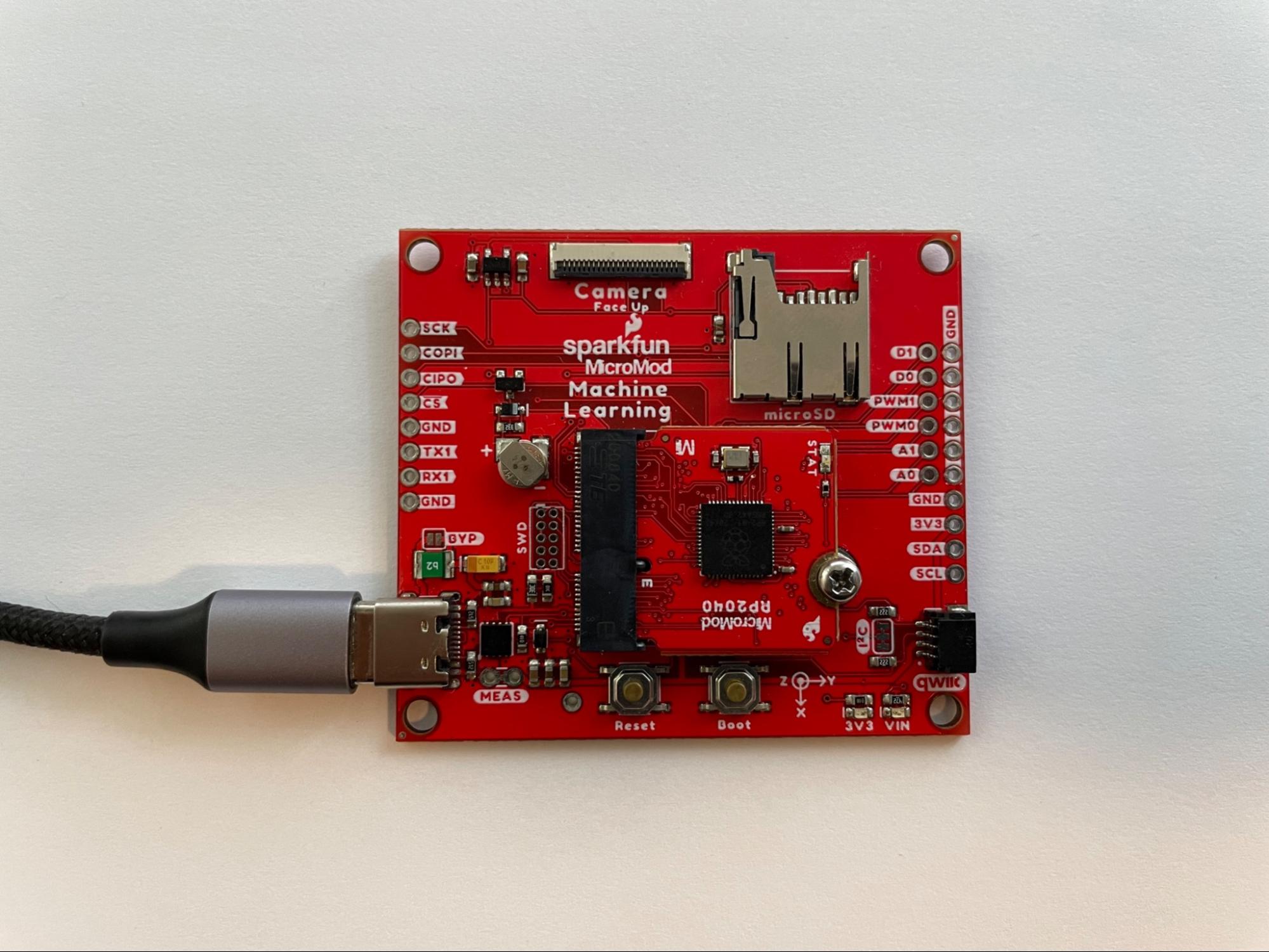
SparkFun RP2040 MicroMod and MicroMod ML Carrier

This board is great for folks new to electronics and microcontrollers. It does not require a soldering iron, knowing how to solder, or how to wire up breadboards.

• SparkFun MicroMod RP2040 Processor. This is the brains of the operation. It contains Raspberry Pi’s RP2040 MCU and 16MB of flash storage.
• SparkFun MicroMod Machine Learning Carrier Board. This enables USB connectivity, and provides a built-in microphone, IMU and camera connector.
• A USB-C cable to connect the board to your computer.
• A Phillips screwdriver.

Raspberry Pi Pico and PDM microphone board

This option is great if you know how to solder (or would like to learn). It requires a soldering iron and knowledge of how to wire a breadboard with electronic components. You’ll need:

• Raspberry Pi Pico.
• Adafruit PDM MEMS Microphone Breakout.
• Half size or full size breadboard.
• Jumper wires.
• A USB-B micro cable to connect the board to your computer.
• Soldering iron.

Both of the options above will allow you to collect real-time 16 kHz audio from a digital microphone and process the audio signal on the development board’s Arm Cortex-M0+ processor, which operates at 125 MHz. The application running on the Arm Cortex-M0+ will have a Digital Signal Processing (DSP) stage to extract features from the audio signal. The extracted features will then be fed into a neural network to perform a classification task to determine if a fire alarm sound is present in the board’s environment.

Dataset

We will start by training a sound classifier (for many events) with TensorFlow using the ESC-50: Dataset for Environmental Sound Classification. After training on this broad dataset, we will use Transfer Learning to fine tune it for our specific audio classification task.

This model will be trained on the ESC-50 dataset, which contains 50 types of sounds. Each sound category has 40 audio files that are 5 seconds each in length. Each audio file will be split into 1 second soundbites, and any soundbites that contain pure silence will be discarded.

A sample waveform from the data set of a dog barking.

Spectrograms

Rather than passing in the time series data directly into our TensorFlow model, we will transform the audio data into an audio spectrogram representation. This will create a 2D representation of the audio signal’s frequency content over time.

The input audio signal we will use will have a sampling rate of 16kHz, this means one second of audio will contain 16,000 samples. Using TensorFlow’s tf.signal.stft(…) function we can transform a 1 second audio signal into a 2D tensor representation. We will choose a frame length of 256 and a frame step of 128, so the output of this feature extraction stage will be a Tensor that has a shape of (124, 129).

An audio spectrogram representation of a dog barking.

The ML model

Now that we have the features extracted from the audio signal, we can create a model using TensorFlow’s Keras API. You can find the complete code linked above. The model will consist of 8 layers:

1. An input layer.
2. A preprocessing layer, that will resize the input tensor from 124x129x1 to 32x32x1.
3. A normalization layer, that will scale the input values between -1 and 1
4. A 2D convolution layer with: 8 filters, a kernel size of 8×8, and stride of 2×2, and ReLU activation function.
5. A 2D max pooling layer with size of 2×2
6. A flatten layer to flatten the 2D data to 1D
7. A dropout layer, that will help reduce overfitting during training
8. A dense layer with 50 outputs and a softmax activation function, which outputs the likelihood of the sound category (between 0 and 1).

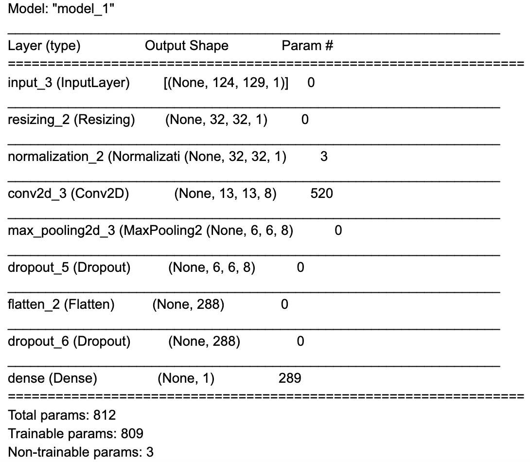
The model summary can be found below:

Notice that this model only has about 15K parameters (this is quite small!)

Fine tuning

Now we will use transfer learning and change the classification head (the last Dense layer) of the model to train a binary classification model for fire alarm sounds. We have collected 10 fire alarm clips from freesound.org and BigSoundBank.com. Background noise clips from the SpeechCommands dataset will be used for non-fire alarm sounds. This dataset is small, and enough for us to get started. Data augmentation techniques will be used to supplement the training data we’ve collected.

For real-world applications, it’s important to collect a much larger dataset (you can learn more about best practices on TensorFlow’s Responsible AI website).

Data Augmentation

Data augmentation is a set of techniques used to increase the size of a dataset. This is done by slightly modifying samples from the dataset or by creating synthetic data. In this situation we are using audio and we will create a few functions to augment different samples. We will use three techniques:

1. Adding white noise to the audio samples.
2. Adding random silence to the audio.
3. Mixing two audio samples together.

As well as increasing the size of the dataset, data augmentation also helps to reduce overfitting by training the model on different (not perfect) data samples. For example, on a microcontroller you are unlikely to have perfect high quality audio, and so a technique like adding white noise can help the model work in situations where your microphone might every so often have noise in there.

A gif showing how data augmentation slightly changes the spectrogram by adding noise (watch it closely, it can be a bit hard to see).

Feature Extraction

TensorFlow Lite for Microcontroller (TFLu) provides a subset of TensorFlow operations, so we are unable to use the tf.signal.sft(…) API we’ve used for feature extraction of the baseline model on our MCU. However, we can leverage Arm’s CMSIS-DSP library to generate spectrograms on the MCU. CMSIS-DSP contains support for both floating-point and fixed-point DSP operations which are optimized for Arm Cortex-M processors, including the Arm Cortex-M0+ that we will be deploying the ML model to. The Arm Cortex-M0+ does not contain a floating-point unit (FPU) so it would be better to leverage a 16-bit fixed-point DSP based feature extraction pipeline on the board.

We can leverage CMSIS-DSP’s Python Wrapper in the notebook to perform the same operations on our training pipeline using 16-bit fixed-point math. At a high level we can replicate the TensorFlow SFT API with the following CMSIS-DSP based operations:

1. Manually creating a Hanning Window of length 256 using the Hanning Window formula along with CMSIS-DSP’s arm_cos_f32 API.
   
2. Creating a CMSIS-DSP arm_rfft_instance_q15 instance and initializing it using CMSIS-DSP’s arm_rfft_init_q15 API.
3. Looping through the audio data 256 samples at a time, with a stride of 128 (this matches the parameters we’ve passed into the TF sft API)
   1. Multiplying the 256 samples by the Hanning Window, using CMSIS-DSP’s arm_mult_q15 API
   2. Calculating the FFT of the output of the previous step, using CMSIS-DSP’s arm_rfft_q15 API
   3. Calculating the magnitude of the previous step, using CMSIS-DSP’s arm_cmplx_mag_q15 API
4. Each audio soundbites’s FFT magnitude represents the one column of the spectrogram.
5. Since our baseline model expects a floating point input, instead of the 16-bit quantized value we were using, the CMSIS-DSP arm_q15_to_float API can be used to convert the spectrogram data from a 16-bit fixed-point value to a floating-point value for training.

The complete Python code for this is a bit long, but can be found in the “Transfer Learning -> Load dataset” section of the Google Colab notebook.

Waveform and audio spectrogram of a smoke alarm sound.

For an in-depth description of how to create audio spectrograms using fixed-point operations with CMSIS-DSP, please see Towards Data Science “Fixed-point DSP for Data Scientists” guide.

Loading the baseline model and changing the classification head

The model we previously trained on the ESC-50 dataset, predicted the presence of 50 sound types, and which resulted in the final dense layer of the model having 50 outputs. The new model we would like to create is a binary classifier, and needs to have a single output value.

We will load the baseline model, and swap out the final dense layer to match our needs:

# We need a new head with one neuron.
model_body = tf.keras.Model(inputs=model.input, outputs=model.layers[-2].output)

classifier_head = tf.keras.layers.Dense(1, activation="sigmoid")(model_body.output)

fine_tune_model = tf.keras.Model(model_body.input, classifier_head)

This results in the following model.summary():

Transfer Learning

Transfer Learning is the process of retraining a model that has been developed for a task to complete a new similar task. The idea is that the model has learned transferable “skills” and the weights and biases can be used in other models as a starting point.

As humans we use transfer learning too. The skills you developed to learn to walk could also be used to learn to run later on.

In a neural network, the first few layers of a model start to perform a “feature extraction” such as finding shapes, edges and colours. The layers later on are used as classifiers; they take the extracted features and classify them.

Because of this, we can assume the first few layers have learned quite general feature extraction techniques that can be applied to similar tasks, and so we can freeze all these layers and use them on a new task in the future. The classifier layer will need to be trained based on the new task.

To do this, we break the process into two steps:

1. Freeze the “backbone” of the model and train the head with a fairly high learning rate. We slowly reduce the learning rate.
2. Unfreeze the “backbone” and fine-tune the model with a low learning rate.

To freeze a layer in TensorFlow we can set layer.trainable=False. Let’s loop through all the layers and do this:

for layer in fine_tune_model.layers:
  layer.trainable = False

and now unfreeze the last layer (the head):

fine_tune_model.layers[-1].trainable = True

We can now train the model using a binary crossentropy loss function. Keras callbacks for early stopping (to avoid overfitting) and a dynamic learning rate scheduler will also be used.

After we’ve trained with the frozen layers, we can unfreeze them:

for layer in fine_tune_model.layers:
  layer.trainable = True

And train again for up to 10 epochs. You can find the complete code for this in the “Transfer Learning -> ”Train Model” section of Colab notebook.

Recording your own training data

We now have an ML model which can classify the presence of fire alarm sound. However this model was trained on publicly available sound recordings which might not match the sound characteristics of the hardware microphone we will use for inferencing.

The Raspberry Pi RP2040 MCU has a native USB feature that allows it to act like a custom USB device. We can flash an application to the board to enable it to act like a USB microphone to our PC. Then we can extend Google Colab’s capabilities with the Web Audio API on a modern Web browser like Google Chrome to collect live data samples (all from within Google Colab!)

Hardware Setup

SparkFun MicroMod RP2040

For assembly, remove the screw on the carrier board, at an angle, slide in the MicroMod RP2040 Processor board into the socket and secure it in place with the screw. See the MicroMod Machine Learning Carrier Board Hookup Guide for more details.

Raspberry Pi Pico

Follow the instructions from the Hardware Setup section of the “Create a USB Microphone with the Raspberry Pi Pico” guide for assembly instructions.

Top: Fritzing wiring diagram Bottom: Assembled breadboard

Setting up the firmware applications toolchains

Rather than setting up the Raspberry Pi Pico’s SDK on your personal computer. We can leverage Colab’s built-in Linux shell command feature to set up the Pico SDK development environment with CMake and GNU Arm Embedded Toolchain.

The pico-sdk will also have to be downloaded to the Colab instance using git:

%%shell
git clone https://github.com/raspberrypi/pico-sdk.git
cd pico-sdk
git submodule init
git submodule update

Compiling and flashing the USB microphone application

Now we can use the USB microphone example from the Microphone Library for Pico. The example application can be compiled using cmake and make. Then we can flash the example application to the board over USB by putting the board into “boot ROM mode” which will allow us to upload an application to the board.

SparkFun

• Plug the USB-C cable into the board and your PC to power the board.
• While holding down the BOOT button on the board, tap the RESET button.

Raspberry Pi Pico

• Plug the USB Micro cable into your PC, but do NOT plug in the Pico side.
• While holding down the white BOOTSEL button, plug in the micro USB cable to the Pico.

If you are using a WebUSB API enabled browser like Google Chrome, you can directly flash the image onto the board from within Google Collab!

Downloading USB microphone application to the board from within Google Colab and WebUSB.

Otherwise, you can manually download the .uf2 file to your computer and then drag it onto the USB disk for the RP2040 board.

Collecting training data

Now that you have flashed the USB microphone application to the board, it will appear as a USB audio input on your PC.

We can now use Google Colab to record a fire alarm sound, select “MicNode ” as the audio input source in the drop down. Then while pressing the test button on a smoke alarm, click the record button on Google Colab to record a 1 second audio clip. Repeat this process a few times.

Similarly, we can also do the same to collect background audio samples in the next code cell in Google Colab. Repeat this a few times for non-fire alarm sounds like silence, yourself talking, or any other normal sounds for the environment.

Final model training

Now that we’ve collected additional samples with the microphone that will be used during inference. We can tune the model again with the new data.

Converting the Model to run on the MCU

We will need to convert the Keras model we’ve used to TensorFlow Lite format so that we can use it for inference on the device.

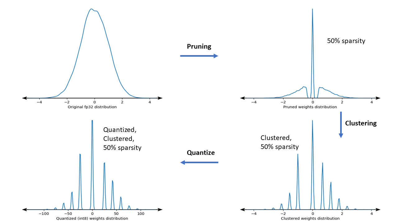
Quantization

To optimize the model to run on the Arm Cortex-M0+ processor, we will use a process called model quantization. Model quantization converts the model’s weights and bias from 32-bit floating point values to 8-bit values. The pico-tflmicro library, which is a port of TFLu for the RP2040’s Pico SDK contains Arm’s CMSIS-NN library, which supports optimized kernel operations for quantized 8-bit weights on Arm Cortex-M processors.

We can use TensorFlow’s Quantization Aware Training (QAT) feature to easily convert the floating-point model to quantized.

Converting the model to TF Lite format

We will now use the tf.lite.TFLiteConverter.from_keras_model(…) API to convert the quantized Keras model to TF Lite format, and then save it to disk as a .tflite file.

converter = tf.lite.TFLiteConverter.from_keras_model(quant_aware_model)
converter.optimizations = [tf.lite.Optimize.DEFAULT]

train_ds = train_ds.unbatch()

def representative_data_gen():
  for input_value, output_value in train_ds.batch(1).take(100):
    # Model has only one input so each data point has one element.
    yield [input_value]
    
converter.representative_dataset = representative_data_gen
# Ensure that if any ops can't be quantized, the converter throws an error
converter.target_spec.supported_ops = [tf.lite.OpsSet.TFLITE_BUILTINS_INT8]
# Set the input and output tensors to uint8 (APIs added in r2.3)
converter.inference_input_type = tf.int8
converter.inference_output_type = tf.int8
tflite_model_quant = converter.convert()

with open("tflite_model.tflite", "wb") as f:
  f.write(tflite_model_quant)

Since TensorFlow also supports loading TF Lite models using tf.lite, we can also verify the functionality of the quantized model and compare its accuracy with the regular unquantized model inside Google Colab.

The RP2040 MCU on the boards we are deploying to, does not have a built-in file system, which means we cannot use the .tflite file directly on the board. However, we can use the Linux `xxd` command to convert the .tflite file to a .h file which can then be compiled in the inference application in the next step.

%%shell
echo "alignas(8) const unsigned char tflite_model[] = {" > tflite_model.h
cat tflite_model.tflite | xxd -i                        >> tflite_model.h
echo "};" 

Deploy the model to the device

We now have a model that is ready to be deployed to the device. We’ve created an application template for inference which can be compiled with the .h file that we’ve generated for the model.

The C++ application uses the pico-sdk as the base, along with the CMSIS-DSP, pico-tflmicro, and Microphone Library for Pico libraries. It’s general structure is as follows:

1. Initialization
   1. Configure the board’s built-in LED for output. The application will map the brightness of the LED to the output of the model. (0.0 LED off, 1.0 LED on with full brightness)
   2. Setup the TF Lite library and TF Lite model for inference
   3. Setup the CMSIS-DSP based DSP pipeline
   4. Setup and start the microphone for real-time audio
2. Inference loop
   1. Wait for 128 * 4 = 512 new audio samples from the microphone
   2. Shift the spectrogram array over by 4 columns
   3. Shift the audio input buffer over by 128 * 4 = 512 samples and copy in the new samples
   4. Calculate 4 new spectrogram columns for the updated input buffer
   5. Perform inference on the spectrogram data
   6. Map the inference output value to the on-board LED’s brightness and output the status to the USB port

In-order to run in real-time each cycle of the inference loop must take under (512 / 16000) = 0.032 seconds or 32 milliseconds. The model we’ve trained and converted takes 24 ms for inference, which gives us ~8 ms for the other operations in the loop.

128 was used above to match the stride of 128 used in the training pipeline for the spectrogram. We used a shift of 4 in the spectrogram to fit within the real-time constraints we had.

Compiling the Firmware

Now we can use CMake to generate the build files required for compilation followed by make to compile.

The “cmake ..” line will have to be changed based on the board you are using:

• SparkFun: cmake .. -DPICO_BOARD=sparkfun_micromod
• Raspberry Pi Pico: cmake .. -DPICO_BOARD=pico

Flashing the Inference Application to the board

You’ll need to put the board into “boot ROM mode” again to load the new application to it.

SparkFun

• Plug the USB-C cable into the board and your PC to power the board.
• While holding down the BOOT button on the board, tap the RESET button.

Raspberry Pi Pico

• Plug the USB Micro cable into your PC, but do NOT plug in the Pico side.
• While holding down the white BOOTSEL button, plug in the micro USB cable to the Pico.

If you are using a WebUSB API enabled browser like Google Chrome, you can directly flash the image onto the board from within Google Colab. Otherwise, you can manually download the .uf2 file to your computer and then drag it onto the USB disk for the RP2040 board.

Monitoring the Inference on the board

Now that the inference application is running on the board you can observe it in action in two ways:

Visually by observing the brightness of the LED on the board. It should remain off or dim when no fire alarm sound is present – and be on when a fire alarm sound is present:

Connecting to the board’s USB serial port to view output from the inference application. If you are using a Web Serial API enabled browser like Google Chrome, this can be done directly from Google Colab:

Improving the model

You now have the first version of the model deployed to the board, and it is performing inference on live 16,000 kHz audio data!

Test out various sounds to see if the model has the expected output. Maybe the fire alarm sound is being falsely detected (false positive) or not detected when it should be (false negative).

If this occurs, you can record more new audio data for the scenario(s) by flashing the USB microphone application firmware to the board, recording the data for training, re-training the model and converting to TF lite format, and re-compiling + flashing the inference application to the board.

Supervised machine learning models can generally only be as good as the training data they are trained with, so additional training data for these scenarios might help. You can also try to experiment with changing the model architecture or feature extraction process – but keep in mind that your model must be small enough and fast enough to run on the RP2040 MCU.

Conclusion

This article covered an end-to-end flow of how to train a custom audio classifier model to run locally on a development board that uses an Arm Cortex-M0+ processor. TensorFlow was used to train the model using transfer learning techniques along with a smaller dataset and data augmentation techniques. We also collected our own data from the microphone that is used at inference time by loading an USB microphone application to the board, and extending Colab’s features with the Web Audio API and JavaScript.

The training side of the project combined Google’s Colab service and Chrome browser, with the open source TensorFlow library. The inference application captured audio data from a digital microphone, used Arm’s CMSIS-DSP library for the feature extraction stage, then used TensorFlow Lite for Microcontrollers with Arm CMSIS-NN accelerated kernels to perform inference with a 8-bit quantized model that classified a real-time 16 kHz audio input on an Arm Cortex-M0+ processor.

The Web Audio API, Web USB API, and Web Serial API features of Google Chrome were used to extend Google Colab’s functionality to interact with the development board. This allowed us to experiment with and develop our application entirely with a web browser and deploy it to a constrained development board for on-device inference.

Since the ML processing was performed on the development boards RP2040 MCU, no audio data left the device at inference time.

Learn more

You can learn more and get hands-on experience using TinyML at the upcoming Arm DevSummit, a 3-day virtual event between October 19 – 21. The event includes workshops on tinyML computer vision for real-world embedded devices and building large vocabulary voice control with Arm Cortex-M based MCUs. We hope to see you there!

Read More

Posted by Jeanine Banks, VP of 3P Core Developer Platforms

At Google we believe that diversity and inclusion are core to innovation, and we know there’s work to be done in improving representation to achieve equity. That’s why we’re excited to announce a new event: The Women in Machine Learning Symposium.

Join us virtually from 9-12 PDT on October 19, 2021, to hear from leaders in the machine learning (ML) industry.

All journeys are different and this event aims to empower the next generation of women leaders in ML. By learning from each other’s stories we want to inspire the creation of a community of support, bringing together women and allies in technology.

We’ll have two keynotes discussing the importance of diversity in ML communities and Open Source Software. You can also hear first-hand the stories and experiences of women who are breaking down barriers and ask them questions live!

Lastly, I invite you to attend one of the breakout sessions tailored to what stage you’re at in your career. From learning how to get started in ML, how to switch from being a tech developer to becoming an ML developer, to learning tips for taking your career to the C-level, this event has a place for you.

RSVP today to reserve your spot and head on over to our website to view the live agenda. I hope to see you there!

Read More

Posted by Wei Wei, TensorFlow Developer Advocate

As the old adage goes, “a picture is worth a thousand words.” Images are rich in visual information, but sometimes the key is with the text within. While it is easy for literate human beings to read words embedded in images, how do we use computer vision and machine learning to teach computers to do so?

Today, we are going to show you how to use TensorFlow Lite to extract text from images on Android devices. We will walk you through the key steps of the Optical Character Recognition (OCR) Android app that we recently open sourced here, which you can refer to for the complete code. You can see how the app extracts the product names from three Google product logos in the animation below.

The process of recognizing text from images is called Optical Character Recognition and is widely used in many domains. For example, Google Maps uses OCR technology to automatically extract information from the geo-located imagery to improve Google Maps.

Generally speaking, OCR is a pipeline with multiple steps. Usually they consist of text detection and text recognition:

• Use a text detection model to find out bounding boxes around text;
• Do some post-processing to transform the bounding boxes;
• Transform the images within those bounding boxes into grayscale, so that a text recognition model can map out the words and numbers.

In our case, we are going to leverage the text detection and text recognition models from TensorFlow Hub. There are several different model versions for speed / accuracy tradeoffs; we use the float16 quantized models here. For more information on model quantization, please refer to the TensorFlow Lite quantization section. We also use OpenCV, which is a widely used computer vision library for Non-Maximum Suppression (NMS) and perspective transformation (we’ll expand on this later) to post-process detection results. In addition, we use the TFLite Support Library to grayscale and normalize the images.

OCR pipeline from text detection, perspective transformation, to recognition.

For text detection, since the detection model accepts a fixed size of 320×320, we use the TFLite Support Library to resize and normalize the input image:

val imageProcessor =
 ImageProcessor.Builder()
   .add(ResizeOp(height, width, ResizeOp.ResizeMethod.BILINEAR))
   .add(NormalizeOp(means, stds))
   .build()
var tensorImage = TensorImage(DataType.FLOAT32)

tensorImage.load(bitmapIn)
tensorImage = imageProcessor.process(tensorImage)

Then we use TFLite to run the detection model:

detectionInterpreter.runForMultipleInputsOutputs(detectionInputs, detectionOutputs)

The output of the detection model is a number of rotated bounding boxes which contain the text in the image. We run Non-Maximum Suppression to identify one bounding box for each text block with OpenCV:

NMSBoxesRotated(
  boundingBoxesMat,
  detectedConfidencesMat,
  detectionConfidenceThreshold.toFloat(),
  detectionNMSThreshold.toFloat(),
  indicesMat
)

Sometimes texts inside images are distorted (e.g., the ‘kubernetes’ sticker on my laptop) with a perspective angle:

Perspective transformation demo

If we just feed the raw rotated bounding box into the recognition model, the model is unlikely to correctly identify the characters. In this case, we need to use OpenCV to do perspective transformation:

val rotationMatrix = getPerspectiveTransform(srcPtsMat, targetPtsMat)

warpPerspective(
  srcBitmapMat,
  recognitionBitmapMat,
  rotationMatrix,
  Size(recognitionImageWidth.toDouble(), recognitionImageHeight.toDouble())
)

After that, we use the TFLite Support Library again to resize, grayscale, and normalize the transformed images inside the bounding boxes:

val imageProcessor =
  ImageProcessor.Builder()
    .add(ResizeOp(height, width, ResizeOp.ResizeMethod.BILINEAR))
    .add(TransformToGrayscaleOp())
    .add(NormalizeOp(mean, std))
    .build()

Finally, we run the text recognition model, map out the characters and numbers from the model output, and update the app UI:

recognitionInterpreter.run(recognitionTensorImage.buffer, recognitionResult)

var recognizedText = ""
for (k in 0 until recognitionModelOutputSize) {
  var alphabetIndex = recognitionResult.getInt(k * 8)
  if (alphabetIndex in 0..alphabets.length - 1)
    recognizedText = recognizedText + alphabets[alphabetIndex]
}
Log.d("Recognition result:", recognizedText)
if (recognizedText != "") {
  ocrResults.put(recognizedText, getRandomColor())
}

That’s it. We are now able to extract text from input images using TFLite within our app.

Finally, if you just want a ready-to-use OCR SDK, Google also offers on-device OCR functionality through ML Kit, which uses TFLite underneath and should be sufficient for most OCR use cases. There are some situations where you may want to build your own OCR solution with TFLite such as:

• You have your own text detection / recognition TFLite models that you would like to use;
• You have special business requirements (e.g. recognizing upside-down text) and need to customize the OCR pipeline;
• You want to support languages not covered by ML Kit;
• Your target user devices that don’t necessarily have Google Play services installed;
• You want to have control over hardware backends (CPU / GPU / etc.) used to run your models.

In these cases, I hope that this tutorial and our example implementation can help you get started on building your own OCR functionality in your app.

You can learn more about OCR with the resources below.

• OpenCV text detection / recognition example
• OCR TFLite community project by @Tulasi123789 and @risingsayak
• OpenCV Text Detection (EAST text detector)
• Keras OCR
• Deep Learning based Text Detection Using OpenCV
• OCR model for reading Captchas with Keras

Acknowledgements

The author would like to thank Tian Lin for the helpful feedback and community contributors @Tulasi123789 and @risingsayak for their prior work on OCR using TFLite (creating and uploading the models to TF Hub, providing accompanying notebooks, and etc.).

Read More

Posted by Sayak Paul (MLE at Carted, and GDE) and Morgan Roff (Google)

We’re happy to share the work completed by Google Summer of Code students working with TensorFlow Hub this year. If you’re a student who is interested in writing open source code, then you’ll likely be interested in Google’s Summer of Code program.

Through this program, students propose project ideas to open source organizations, and if selected, receive a stipend to work with them to complete their projects over the summer. Students have the opportunity to learn directly from mentors within their selected organization, and organizations benefit from the students’ contributions. This year, 17 successful students completed their projects with the TensorFlow organization on many projects. In this article, we’ll focus on some of the work completed on TensorFlow Hub.

We’re Sayak and Morgan, two mentors for projects on TensorFlow Hub (TF Hub). Here we share what the students learned about building and publishing state-of-the-art models, training them on large-scale benchmark datasets, what we learned as mentors, and how rewarding summer of code was for each of us, and for the community.

We had the opportunity to mentor two students – Aditya Kane and Vasudev Gupta. Aditya successfully implemented several variants of RegNets including one based on this paper, and trained them on the ImageNet-1k dataset. Vasudev ported the pre-trained wav2vec2 weights from this paper to TensorFlow, which required him to implement the model architecture from scratch. He then demonstrated fine-tuning these pre-trained checkpoints on the LibriSpeech dataset, making his work more customizable and relevant for the community.

With model training happening at such a large scale, it becomes especially important to follow good engineering practices during the implementation. These include code modularization, unit tests, good design patterns, optimizations, and so on. Models were trained on Cloud TPUs to accelerate training time, and as such, substantial effort was put into the data input pipelines to ensure maximum accelerator utilization.

All of these factors collectively contributed to the complexity of the projects. Thanks to the Summer of Code program, students have the opportunity to tackle these challenges with the help of experienced mentors. This also enables students to gain insight into their organizations, and interact with people with many skillsets who cooperate to make large projects possible. A big thank you here to our students, who gracefully handled this engineering work and listened to our feedback.

Vasudev and Aditya contributed significant pre-trained models to TensorFlow Hub, along with tutorials (Wav2Vec, RegNetY) on their use, and TensorFlow implementations for folks who want to dig deeper. In their own words:

The last 2-3 months were full of lots of learning and coding. GSoC helped me get into the speech domain and motivated me to explore more about the TensorFlow ecosystem. I am thankful to my mentors for their continuous & timely feedback. I am looking forward to contributing more to the TensorFlow community and other awesome open source projects out there. – Vasudev Gupta

More about RegNets and Wav2Vec2

Almost 6 years after they were first published, ResNets are still widely used as benchmark architectures across image understanding tasks. Many recent self-supervised and semi-supervised learning frameworks still leverage ResNet50 as their backbone architectures. However, ResNets often do not scale well under larger data regimes and suffer from large training and inference time latencies as they grow. In contrast, RegNets were developed specifically to be a scalable architecture framework that maintains low latency while demonstrating high performance on standard image recognition tasks. Aditya’s models are published on TF Hub, with code and tutorials on GitHub.

Self-supervised learning is an important area of machine learning research. Many recent success stories have been focused on NLP and Computer Vision, and for Vasudev’s project, we wanted to explore speech. Last year, a group of researchers released the wav2vec2 framework for learning representations from audio in a self-supervised manner, benefiting downstream tasks like speech-to-text.

Using wav2vec2, you can now pre-train speech models without labeled data, and fine-tune those models on downstream tasks like speaker recognition. Vasudev’s models are available on TF Hub, along with a new tutorial on fine-tuning, and code on GitHub.

Wrapping up

We’d like to say a heartfelt thank you to all the students, mentors, and organizers who made Summer of Code a success despite this year’s many challenges. We encourage you to check out these models and share what you have built with us by tagging #TFHub on your social media posts, or share your work for the community spotlight program. If you have questions or want to learn more about these new models, you can ask them on discuss.tensorflow.org.

Read More

Posted by Gal Moran, Iris Shmuel, and Daniel Marcous (Data Scientists at Waze)

Waze

Waze is the world’s largest community-based traffic and navigation app. It uses real-time data to help users circumvent literal and figurative bumps in the road. On top of mobile navigation, Waze offers a web platform, a carpool app, partnership services, an advertisement platform and more. Such a broad portfolio brings along diverse technological challenges and many different use cases.

ML @Waze

Waze relies on many ML solutions, including:

• Predicting ETA
• Matching Riders & Drivers (Carpool)
• Serving The Right Ads

But it’s not that easy to get something like these right and “production grade”. It is very common for these kinds of projects to have requirements for complex surrounding infrastructure for getting them to production and hence require multiple engineers (data scientist, software engineer and software reliability engineers) and a lot of time. Even more so when you mix in the Waze-y requirements like large scale data, low (real-time, actually) latency inference, diverse use cases, and a whole lot of geospatial data.

The above is a good reason why opportunistically starting to do ML created a chaotic state at Waze. For us it manifested as:

• Multiple ML frameworks – you name it (sklearn, xgboost, TensorFlow, fbprophet, Java PMML, hand made etc.)
• ML & Ops disconnect – models & feature engineering embedded in (Java) backend servers by engineers with limited monitoring and validation capabilities
• Semi-manual operations for training, validation and deployment
• A hideously long development cycle from idea to production

Overall, data scientists ended up spending a lot of their time on ops and monitoring instead of focusing on the actual modelling and data processing. At a certain level of growth we’ve decided to organize the chaos and invest in automation and processes so we can scale faster. We’ve decided to heavily invest in a way to dramatically increase velocity and quality by adopting a full cycle data science philosophy. This means that in this new world we wanted to build, a single data scientist is able to close the product cycle from research to a production grade service.

Data scientists now directly contribute to production to maximize impact. They focus on modelling and data processing and get many infrastructures and ops work out-of-the-box. While we are not yet at the end of this journey fully realizing the above vision, we feel like the effort layed out here was crucial in putting us on the right track.

Waze’s ML Stack

Translating the above philosophy to a tech spec, we were set on creating an easy, stable, automated and uniform way of building ML pipelines at Waze.

Deep diving into tech requirements we came up with the below criteria:

• Simple — to understand, use, operate
• Managed — no servers, no hardware, just code
• Customizable — get the simple stuff for free, yet flexible enough to go crazy for the 5% that would require going outside the lines
• Scalable — auto scalable data processing, training, inference
• Pythonic — we need something production-ready, that works with most tools and code today and fits the standard data scientist. There are practically no other options than Python these days.

For the above reasons we’ve landed on TFX and the power of its built-in components to deliver these capabilities mostly out of the box.

It’s worth saying – Waze runs its tech stack on Google Cloud Platform (GCP).

It happens to be that GCP offers a suite of tools called Vertex AI. It is the ML infrastructure platform Waze is building on top of. While we use many components of Vertex AI’s managed services, we will focus here on – Vertex Pipelines – a framework for ML pipelines that helps us encapsulate TFX (or any pipeline) complexity and setup.

Together with our data tech stack, the overall ML architecture at Waze (all managed, scaled, pythonic etc.) is as follows:

Careful readers will notice the alleged caveat here – we go all in on TensorFlow.

TFX means TensorFlow (even though that’s not exactly true anymore, let’s assume it is).

It might be a little scary at first when you have many different use cases.

Fortunately, the TF ecosystem is rich and Waze has the merit of having large enough data that neural nets converge.

Since starting this we’ve yet to find a use case that TF magic does not solve better or adequately as other frameworks (and not talking about micro % points, not trying to do a Kaggle competition here but get something to production).

Waze TFX

You might think that landing on TFX and Vertex Pipelines solved all our problems, but that’s not exactly true.

In order to make things truly simple we’ve had to write some “glue code” (integrating the various products in the above architecture diagram) and abstracting enough details so the common data scientist could use this stuff effectively and fast.

That resulted in:

• Eliminated boilerplate
• Hiding all common TFX components so data scientists only focus on feature engineering and modelling and get the entire pipeline for free
• Generating BigQuery based train / eval split
• Providing pre-implemented optional common features transform (e.g. scaling, normalization, imputations)
• Providing pre-implemented Keras models (e.g. DNN/RNN model. TF Estimator like but in Keras that speaks TFX)
• Utility functions (e.g. TF columns preparation)
• Unit testing framework for tf.transform feature engineering code
• Orchestrated and scheduled pipeline runs from Airflow using a Cloud run instance with all TFX packages installed (without installing it on the Airflow composer)

We’ve put it all in an easy to use Python package called “waze-data-tfx”

On top, we provided a super detailed walkthrough, usage guides and code templates, to our data scientists, so the common DS workflow is: fork, change config, tweak the code a little, deploy.

For reference this is how a simple waze-data-tfx pipeline looks like:

1. Configuration

   _DATASET_NAME = 'tfx_examples'
   _TABLE_NAME = 'simple_template_data'
   
   _LABEL_KEY = 'label'
   _CATEGORICAL_INT_FEATURES = {
      "categorical_calculated": 2,
   }
   _DENSE_FLOAT_FEATURE_KEYS = ["numeric_feature1", "numeric_feature2"]
   _BUCKET_FEATURES = {
      "numeric_feature1": 5,
   }
   _VOCAB_FEATURES = {
      "categorical_feature": {
          'top_k': 5,
          'num_oov_buckets': 3
      }
   }
   
   _TRAIN_BATCH_SIZE = 128
   _EVAL_BATCH_SIZE = 128
   _NUM_EPOCHS = 250
   
   _TRAINING_ARGS = {
      'dnn_hidden_units': [6, 3],
      'optimizer': tf.keras.optimizers.Adam,
      'optimizer_kwargs': {
          'learning_rate': 0.01
      },
      'layer_activation': None,
      'metrics': ["Accuracy"]
   }
   
   _EVAL_METRIC_SPEC = create_metric_spec([
      mse_metric(upper_bound=25, absolute_change=1),
      accuracy_metric()
   ])

2. Feature Engineering

   def preprocessing_fn(inputs):
      """tf.transform's callback function for preprocessing inputs.
   
      Args:
          inputs: map from feature keys to raw not-yet-transformedfeatures.
   
      Returns:
          Map from string feature key to transformed feature operations.
      """
      outputs = features_transform(
          inputs=inputs,
          label_key=_LABEL_KEY,
          dense_features=_DENSE_FLOAT_FEATURE_KEYS,
          vocab_features=_VOCAB_FEATURES,
          bucket_features=_BUCKET_FEATURES,
      )
      return outputs

3. Modelling

   def _build_keras_model(**training_args):
      """Build a keras model.
   
      Args:
          hidden_units: [int], the layer sizes of the DNN (input layer first).
          learning_rate: [float], learning rate of the Adam optimizer.
   
      Returns:
          A keras model
      """
      feature_columns = 
          prepare_feature_columns(
              dense_features=_DENSE_FLOAT_FEATURE_KEYS,
              vocab_features=_VOCAB_FEATURES,
              bucket_features=_BUCKET_FEATURES,
          )
   
      return _dnn_regressor(deep_columns=list(feature_columns.values()),
                            dnn_hidden_units=training_args.get(
                                "dnn_hidden_units"),
                            dense_features=_DENSE_FLOAT_FEATURE_KEYS,
                            vocab_features=_VOCAB_FEATURES,
                            bucket_features=_BUCKET_FEATURES,
                            )

4. Orchestration

   pipeline_run = WazeTFXPipelineOperator(
      dag=dag,
      task_id='pipeline_run',
      model_name='basic_pipeline_template',
      package=tfx_pipeline_basic,
      pipeline_project_id=EnvConfig.get_value('gcp-project-infra'),
      table_project_id=EnvConfig.get_value('gcp-project-infra'),
      project_utils_filename='utils.py',
      gcp_conn_id=gcp_conn_id,
      enable_pusher=True,
   )

Simple, right?

When you commit a configuration file to the code base it gets deployed and sets up continuous training, and a full blown pipeline including all TFX and Vertex AI magics like data validation, transforms deployed to Dataflow, monitoring etc.

Summary

We knew we were up to something good when one of our data scientists came back from a long leave and had to use this new framework for a use case. She said that she was able to spin up a full production-ready pipeline in hours, something that before her leave would have taken her weeks to do.

Going forward we have much planned that we want to bake into `waze-data-tfx`. A key advantage that we see in having this common infrastructure is that once a feature is added, then everyone can enjoy it “for free”. For example, we plan on adding additional components to the pipeline, such as Infra Validator and Fairness Indicators. Once these are supported, every new or existing ML pipeline will add these components out-of-the-box, no extra code needed.

Additional improvements we are planning are around deployment. We wish to provide deployment quality assurance while automating as much as possible.

One way we are currently exploring doing so is using canary deployments. A data scientist will simply need to configure an evaluation metric and the framework (using Vertex Prediction traffic splitting capabilities and other continuous evaluation magic) would test the new model in production and gradually deploy or rollback according to the evaluated metrics.

Read More

Posted by Elie Bursztein and Owen Vallis, Google

Today we are releasing the first version of TensorFlow Similarity, a python package designed to make it easy and fast to train similarity models using TensorFlow.

Examples of nearest neighbor searches performed on the embeddings generated by a similarity model trained on the Oxford IIIT Pet Dataset

The ability to search for related items has many real world applications, from finding similar looking clothes, to identifying the song that is currently playing, to helping rescue missing pets. More generally, being able to quickly retrieve related items is a vital part of many core information systems such as multimedia searches, recommender systems, and clustering pipelines.

Similarity models learn to output embeddings that project items in a metric space where similar items are close together and far from dissimilar ones

Under the hood, many of these systems are powered by deep learning models that are trained using contrastive learning. Contrastive learning teaches the model to learn an embedding space in which similar examples are close while dissimilar ones are far apart, e.g., images belonging to the same class are pulled together, while distinct classes are pushed apart from each other. In our example, all the images from the same animal breed are pulled together while different breeds are pushed apart from each other.

Oxford-IIIT Pet dataset visualization using the Tensorflow Similarity projector

When applied to an entire dataset, contrastive losses allow a model to learn how to project items into the embedding space such that the distances between embeddings are representative of how similar the input examples are. At the end of training you end up with a well clustered space where the distance between similar items is small and the distance between dissimilar items is large. For example, as visible above, training a similarity model on the Oxford-IIIT Pet dataset leads to meaningful clusters where similar looking breeds are close-by and cats and dogs are clearly separated.

Finding related items involve computing the query image embedding, performing an ANN search to find similar items and fetching similar items metadata including the images bytes.

Once the model is trained, we build an index that contains the embeddings of the various items we want to make searchable. Then at query time, TensorFlow Similarity leverages Fast Approximate Nearest Neighbor search (ANN) to retrieve the closest matching items from the index in sub-linear time. This fast look up leverages the fact that TensorFlow Similarity learns a metric embedding space where the distance between embedded points is a function of a valid distance metric. These distance metrics satisfy the triangle inequality, making the space amenable to Approximate Nearest Neighbor search and leading to high retrieval accuracy.

Other approaches, such as using model feature extraction, require the use of an exact nearest neighbor search to find related items and may not be as accurate as a trained similarity model. This prevents those methods scaling as performing an exact search requires a quadratic time in the size of the search index. In contrast, TensorFlow Similarity’s built-in Approximate Nearest Neighbor indexing system, which relies on the NMSLIB, makes it possible to search over millions of indexed items, retrieving the top-K similar matches within a fraction of second.

Beside accuracy and retrieval speed, the other major advantage of similarity models is that they allow you to add an unlimited new number of classes to the index without having to retrain. Instead you only need to compute the embeddings for representative items of the new classes and add them to the index. This ability to dynamically add new classes is particularly useful when tackling problems where the number of distinct items is unknown ahead of time, constantly changing, or is extremely large. An example of this would be enabling users to discover newly released music that is similar to songs they have liked in the past.

TensorFlow Similarity provides all the necessary components to make similarity training evaluation and querying intuitive and easy. In particular, as illustrated below, TensorFlow Similarity introduces the SimilarityModel(), a new Keras model that natively supports embedding indexing and querying. This allows you to perform end-to-end training and evaluation quickly and efficiently..

A minimal example that trains, indexes and searches on MNIST data can be written in less than 20 lines of code:

from tensorflow.keras import layers

# Embedding output layer with L2 norm
from tensorflow_similarity.layers import MetricEmbedding 
# Specialized metric loss
from tensorflow_similarity.losses import MultiSimilarityLoss 
# Sub classed keras Model with support for indexing
from tensorflow_similarity.models import SimilarityModel
# Data sampler that pulls datasets directly from tf dataset catalog
from tensorflow_similarity.samplers import TFDatasetMultiShotMemorySampler
# Nearest neighbor visualizer
from tensorflow_similarity.visualization import viz_neigbors_imgs


# Data sampler that generates balanced batches from MNIST dataset
sampler = TFDatasetMultiShotMemorySampler(dataset_name='mnist', classes_per_batch=10)

# Build a Similarity model using standard Keras layers
inputs = layers.Input(shape=(28, 28, 1))
x = layers.Rescaling(1/255)(inputs)
x = layers.Conv2D(64, 3, activation='relu')(x)
x = layers.Flatten()(x)
x = layers.Dense(64, activation='relu')(x)
outputs = MetricEmbedding(64)(x)

# Build a specialized Similarity model
model = SimilarityModel(inputs, outputs)

# Train Similarity model using contrastive loss
model.compile('adam', loss=MultiSimilarityLoss())
model.fit(sampler, epochs=5)

# Index 100 embedded MNIST examples to make them searchable
sx, sy = sampler.get_slice(0,100)
model.index(x=sx, y=sy, data=sx)

# Find the top 5 most similar indexed MNIST examples for a given example
qx, qy = sampler.get_slice(3713, 1)
nns = model.single_lookup(qx[0])

# Visualize the query example and its top 5 neighbors
viz_neigbors_imgs(qx[0], qy[0], nns)

Even though the code snippet above uses a sub-optimal model, it still yields good matching results where the nearest neighbors clearly looks like the queried digit as visible in the screenshot below:

This initial release focuses on providing all the necessary components to help you build contrastive learning based similarity models, such as losses, indexing, batch samplers, metrics, and tutorials. TF Similarity also makes it easy to work with the Keras APIs and use the existing Keras Architectures. Moving forward, we plan to build on this solid foundation to support semi-supervised and self-supervised methods such as BYOL, SWAV, and SimCLR.

You can start experimenting with TF Similarity right away by heading to the Hello World tutorial. For more information you can check out the project Github.

Read More

Posted by Marat Dukhan and Frank Barchard, software engineers

Quantization is among the most popular methods to speedup neural network inference on CPUs. A year ago TensorFlow Lite increased performance for floating-point models with the integration of XNNPACK backend. Today, we are extending the XNNPACK backend to quantized models with, on average across computer vision models, 30% speedup on ARM64 mobile phones, 5X speedup on x86-64 laptop and desktop systems, and 20X speedup for in-browser inference with WebAssembly SIMD compared to the default TensorFlow Lite quantized kernels.

Quantized inference in XNNPACK is optimized for symmetric quantization schemas used by the TensorFlow Model Optimization Toolkit. XNNPACK supports both the traditional per-tensor quantization schema and the newer accuracy-optimized schema with per-channel quantization of weights and per-tensor quantization of activations. Additionally, XNNPACK supports the asymmetric quantization schema, albeit with reduced efficiency.

Performance improvements

We evaluated XNNPACK-acclerated quantized inference on a number of edge devices and neural network architectures. Below, we present benchmarks on four public and two internal quantized models covering common computer vision tasks:

1. EfficientNet-Lite0 image classification [download]
2. EfficientDet-Lite0 object detection [download]
3. DeepLab v3 segmentation with MobileNet v2 feature extractor [download]
4. CartoonGAN image style transfer [download]
5. Quantized version of the Face Mesh landmarks
6. Quantized version of the Video Segmentation

Speedup from XNNPACK on single-threaded inference of quantized computer vision models on Android/ARM64 mobile phones.

Across the six Android ARM64 mobile devices XNNPACK delivers, on average, 30% speedup over the default TensorFlow Lite quantized kernels.

Speedup from XNNPACK on single-threaded inference of quantized computer vision models on x86-64 laptop and desktop systems.

XNNPACK offers even greater improvements on laptop and desktop systems with x86 processors. On the 5 x86 processors in our benchmarks XNNPACK accelerated inference on average by 5 times. Notably, low-end and older processors which don’t support AVX instructions see over 20X speedup from switching quantized inference to XNNPACK: while the previous TensorFlow Lite inference backend had optimized implementations only for AVX, AVX2, and AVX512 instruction sets, XNNPACK provides optimized implementations for all x86-64 processors.

Speedup from XNNPACK on single-threaded WebAssembly SIMD inference of quantized computer vision models on mobile phones, laptops, and desktops when running through V8.

Besides the traditional mobile and laptop/desktop platforms, XNNPACK brings accelerated quantized inference to the Web platform through the TensorFlow Lite Web API. The above plot demonstrates a geomean speedup of 20X over the default TensorFlow Lite implementation when running WebAssembly SIMD benchmarks through the V8 JavaScript engine on 3 x86-64 and 2 ARM64 systems.

Two years of optimizations

XNNPACK started its life as a fork of QNNPACK library, but as the first version of XNNPACK focused on floating-point inference and QNNPACK focused on quantized inference, it was not possible to compare the two. Now with XNNPACK introducing support for quantized inference, we can directly evaluate and attribute the two further years of performance optimizations.

To compare the two quantized inference backends, we ported randomized MobileNet v1 and MobileNet v2 models from XNNPACK API to QNNPACK API, and benchmarked their single-threaded performance on two ARM64 Android phones and two x86-64 systems. The results are presented in the plot above, and the progress made by XNNPACK in two years is striking. XNNPACK is 50% faster on the older Pixel 3a phone and 4-5X faster on the newer Pixel 4a phone, 2.5X faster on the x86-64 laptop, and over 3X faster on the x86-64 workstation. These improvements are the result of a multiple optimizations XNNPACK gained in the two years since it forked from QNNPACK:

• XNNPACK retained the optimizations in QNNPACK, like the Indirect Convolution algorithm and microarchitecture-specific microkernel selection, and further augmented them with Indirect Deconvolution algorithm, and more flexible capabilities, like built-in numpy-like broadcasting in the quantized addition and quantized multiplication operators.
• Convolution, Deconvolution, and Fully Connected operators accumulate products of 8-bit activations and weights into a 32-bit number, and in the end this number needs to be converted back, or requantized, to an 8-bit number. There are multiple ways how requantization can be implemented, but QNNPACK adapted schema from the GEMMLOWP library, which pioneered quantized computations for neural network inference. However, it has since been discovered that GEMMLOWP requantization schema is suboptimal in terms of both accuracy and performance, and XNNPACK replaced it with more performant and accurate alternatives
• Whereas QNNPACK targeted asymmetric quantization schema, where both activations and weights are represented as unsigned integers with zero point and scale quantization parameters, XNNPACK’s optimizations focus on symmetric quantization, where both activations and weights are signed integers, and weights have additional restrictions: the zero point of the weights is always zero and the quantized weights elements are limited to the [-127, 127] range (-128 is excluded even though it can be represented as a signed 8-bit integer). Symmetric quantization offers two computational advantages exploited in XNNPACK. First, when the filter weights are static, the results of accumulating the product of input zero point by the filter weights can be completely fused into the bias term in the Convolution, Deconvolution, and Fully Connected operators. Thus, zero point parameters are completely absent from the inference computations. Secondly, the product of a signed 8-bit input element by the weight element restricted to [-127, 127] fits into 15 bits. This enables the microkernels for Convolution, Deconvolution, and Fully Connected operators to do half of the accumulations on 16-bit variables rather than always extending the products to 32 bits.
• QNNPACK microkernels were optimized NEON SIMD instructions on ARM and SSE2 SIMD instructions on x86, but XNNPACK supports a much wider set of instruction set-specific optimizations. Most quantized microkernels in XNNPACK are optimized for SSE2, SSE4.1, AVX, XOP, AVX2, and AVX512 instructions on x86/x86-64, for NEON, NEON V8, and NEON dot product instructions on ARM/ARM64, and for WebAssembly SIMD instructions. Additionally, XNNPACK provides scalar implementations for WebAssembly 1.0 and pre-NEON ARM processors.
• QNNPACK introduced the idea of specialized assembly microkernels for high-end ARM and low-end ARM cores, but XNNPACK takes this idea much further. XNNPACK not only includes specialized expert-tuned software pipelined assembly microkernels for Cortex-A53, Cortex-A55, and high-end cores with and without NEON dot product instructions, but even supports switching between them on the fly. When a thread doing inference migrates from a big to a little core, XNNPACK automatically adapts from using a microkernel optimized for the big core to the one optimized for the little core.
• QNNPACK mainly focused on multi-threaded inference and organized computations as a large number of small tasks, each computing a tiny tile of the output tensor. XNNPACK reworked parallelisation and made the tasks flexible: they can be fine-grained or coarse-grained depending on the number of threads participating in the parallelization. Through dynamic adjustment of task granularity, XNNPACK archives low overhead in single-threaded execution and high parallelization efficiency for multi-threaded inference.

Taken together, these optimizations make XNNPACK the new state-of-art for quantized inference, and turn TensorFlow Lite into the most versatile quantized inference solution, covering systems from Raspberry Pi Zero to Chromebooks to workstations with server-class processors.

How can you use it?

Quantized XNNPACK inference is enabled by default in the CMake builds of TensorFlow Lite for all platforms, in the Bazel builds of TensorFlow Lite for the Web platform, and will be available in TensorFlow Lite Web API in the 2.7 release. In Bazel builds for other platforms, quantized XNNPACK inference is enabled via a build-time opt-in mechanism. When building TensorFlow Lite with Bazel, add --define tflite_with_xnnpack=true --define xnn_enable_qs8=true, and the TensorFlow Lite interpreter will use the XNNPACK backend by default for supported operators with symmetric quantization. Limited support for operators with asymmetric quantization is available via the --define xnn_enable_qu8=true Bazel option.

Which operations are accelerated?

The XNNPACK backend currently supports a subset of quantized TensorFlow Lite operators (see documentation for details and limitations). XNNPACK supports models produced by the Model Optimization Toolkit through post-training integer quantization and quantization-aware training, but not post-training dynamic range quantization.

Future work

This is the third version of the XNNPACK integration into TensorFlow Lite following the initial release of the floating-point implementation and the subsequent release that brought sparse inference support. In the following versions we plan to add the following improvements:

• Half-precision inference on the recent ARM processors
• Sparse quantized inference.
• Even faster dense inference.

We encourage you to leave your thoughts and comments on our GitHub and StackOverflow pages, and you can ask questions on discuss.tensorflow.org

Read More

Posted by Luiz GUStavo Martins, Developer Advocate

At Google I/O, we shared a set of tutorials to help you use machine learning on audio. In this blog post you’ll find resources to help you develop and customize an audio classification model for your app, and a couple of real world examples for inspiration.

Machine learning for audio

Sound and audio are sometimes used interchangeably, but they have a key difference. Sound is in essence what you can hear while audio is the sound’s electronic representation. That’s why we usually use the term audio when talking about machine learning.

Machine Learning for audio can be used to:

• Understand speech
• Understand musical instruments
• Classify events (which bird is that?)
• Detect pitch
• Generate music

In this post we will focus on audio classification of events, a common scenario in practice with many real world applications like NOAA creating a humpback whale acoustic detector, and the Zoological Society of London using audio recognition to protect wildlife.

A number of classification models are available for you to try right now on TensorFlow Hub (YAMNet, Whale detection).

Audio recognition can also run completely on-device. For example, Android has a sound notifications feature that provides push notification for important sounds around you. It can also detect which music is playing, or even help with an ML-powered audio recorder app that can transcribe conversations on-device.

Having the models is only the beginning. Now you might ask:

• How do I use them on my app?
• How do I customize them for my audio use case?

Deploying machine learning models on-device

Imagine you have an audio classification model ready, such as a pretrained one from TF-Hub, how would you use this in a mobile app? To help you integrate audio classification into your app we created the TensorFlow Lite Task Library. The Audio Classifier component was released and you only need a couple of lines of code to add audio classification to your application:

// Initialization
val classifier = AudioClassifier.createFromFile(this, modelPath)

// Start recording
val record = classifier.createAudioRecord()
record.startRecording()

// Load latest audio samples
val tensor = classifier.createInputTensorAudio()
tensor.load(record);

// Run inference
val output = classifier.classify(tensor)

The library takes care of loading the model to memory, to create the audio recorder with the proper model specifications (sample rate, bit rate) and the classification method to get the model’s inference results. Here you can find a full sample to get some inspiration.

Customizing the models

What if you need to recognize audio events that are not in the set provided by the pretrained models? Or if you need to specialize them to fewer classes? In these situations, you need to fine tune the model using a technique called Transfer Learning.

This is a very popular process and you don’t need to be an expert on machine learning to be able to do it. You can use Model Maker to help you with this.

spec = audio_classifier.YamNetSpec()
data = audio_classifier.DataLoader.from_folder(spec, DATA_DIR)
 
train_data, validation_data = data.split(0.8)
model = audio_classifier.create(train_data, spec, validation_data)
 
model.export(models_path)

You can find complete code here. The output model can be directly loaded by the Task Library. And Model Maker can customize models not only for audio but also for image, text and recommendation system

Summary

Machine learning for audio is an exciting field and with many possibilities, enabling many new features. Doing ML on-device is getting easier and faster with tools like TensorFlow Lite Task Library and customization can be done without expertise in the field with Model Maker.

You can learn more about it on our new On-Device Machine Learning website (the audio path is here). You’ll find tutorials, codelabs and lots of resources on how to do not only audio related tasks but also for image (classification, object detection) and text (classification, entity extraction, question and answer)

You can share with us what you build by adding #TensorFlow on your social network post with your project, or submit it for the TensorFlow community spotlight program. And if you have any questions, you can ask them on discuss.tensorflow.org.

Read More

Posted by Ivan Grishchenko, Valentin Bazarevsky, Eduard Gabriel Bazavan, Na Li, Jason Mayes, Google

Pose detection is an important step in understanding more about the human body in videos and images. Our existing models have supported 2D pose estimation for some time, which many of you may have already tried.

Today, we are launching our first 3D model in TF.js pose-detection API. 3D pose estimation opens up new design opportunities for applications such as fitness, medical, motion capture and beyond – in many of these areas we’ve seen a growing interest from the TensorFlow.js community. A great example of this is 3D motion capture to drive a character animation in the browser.

3D motion capture with BlazePose GHUM by Richard Yee (used with permission, live demo available at 3d.kalidoface.com)

This community demo uses multiple models powered by MediaPipe and TensorFlow.js (namely FaceMesh, BlazePose and HandPose). Even better, no app install is needed as you just need to visit a webpage to enjoy the experience. So with that in mind, let’s learn more and see this new model in action!

Try out the live demo!

Installation

The pose-detection API provides two runtimes for BlazePose GHUM, namely MediaPipe runtime and TensorFlow.js runtime.

To install the API and runtime library, you can either use the <script> tag in your html file or use NPM.

Through script tag:

<script src="https://cdn.jsdelivr.net/npm/@tensorflow-models/pose-detection"></script>
<!-- Include below scripts if you want to use TF.js runtime. -->
<script src="https://cdn.jsdelivr.net/npm/@tensorflow/tfjs-core"></script>
<script src="https://cdn.jsdelivr.net/npm/@tensorflow/tfjs-converter"></script>
<script src="https://cdn.jsdelivr.net/npm/@tensorflow/tfjs-backend-webgl"></script>

<!-- Optional: Include below scripts if you want to use MediaPipe runtime. -->
<script src="https://cdn.jsdelivr.net/npm/@mediapipe/pose"></script>

Through NPM:

yarn add @tensorflow-models/pose-detection

# Run below commands if you want to use TF.js runtime.
yarn add @tensorflow/tfjs-core @tensorflow/tfjs-converter
yarn add @tensorflow/tfjs-backend-webgl

# Run below commands if you want to use MediaPipe runtime.
yarn add @mediapipe/pose

To reference the API in your JS code, it depends on how you installed the library.

If installed through script tag, you can reference the library through the global namespace poseDetection.

If installed through NPM, you need to import the libraries first:

import * as poseDetection from '@tensorflow-models/pose-detection';
// Uncomment the line below if you want to use TF.js runtime.
// import '@tensorflow/tfjs-backend-webgl';
// Uncomment the line below if you want to use MediaPipe runtime.
// import '@mediapipe/pose';

Try it yourself!

First, you need to create a detector:

const model = poseDetection.SupportedModels.BlazePose;
const detectorConfig = {
  runtime: 'mediapipe', // or 'tfjs'
  modelType: 'full'
};
detector = await poseDetection.createDetector(model, detectorConfig);

Choose a modelType that fits your application needs, there are three options for you to choose from: lite, full, and heavy. From lite to heavy, the accuracy increases while the inference speed decreases. Please try our live demo to compare different configurations.

Once you have a detector, you can pass in a video stream to detect poses:

const video = document.getElementById('video');
const poses = await detector.estimatePoses(video);

How to use the output? poses represent an array of detected pose predictions in the image frame. For each pose, it contains keypoints and keypoints3D. The keypoints are the same as the 2D model we launched before, it is an array of 33 keypoint objects, each object has x, y in pixel units.

keypoints3D is an additional array with 33 keypoint objects, each object has x, y, z. The x, y, z are in meter units. The person is modeled as if they were in a 2m x 2m x 2m cubic space. The range for each axis goes from -1 to 1 (therefore 2m total delta). The origin of this 3D space is the hip center (0, 0, 0). From the origin, z is positive if moving closer to the camera, and negative if moving away from the camera. See below output snippet for example:

[
  {
    score: 0.8,
    keypoints: [
      {x: 230, y: 220, score: 0.9, name: "nose"},
      {x: 212, y: 190, score: 0.8, name: "left_eye"},
      ...
    ],
    keypoints3D: [
      {x: 0.5, y: 0.9, z: 0.06 score: 0.9, name: "nose"},
      ...
    ]
  }
]

You can refer to our ReadMe for more details about the API.

As you begin to play and develop with BlazePose GHUM, we would appreciate your feedback and contributions. If you make something using this model, tag it with #MadeWithTFJS on social media so we can find your work, as we would love to see what you create.

Model deep dive

The key challenge to build the 3D part of our pose model was obtaining realistic, in-the-wild 3D data. In contrast to 2D, which can be obtained via human annotation, accurate manual 3D annotation becomes a uniquely challenging task. It requires either a lab setup or specialised hardware with depth sensors for 3D scans – which introduce additional challenges to preserve a good level of human and environment diversity in the dataset. Another alternative, which many researchers choose – to build a completely synthetic dataset, which introduces yet another challenge of domain adaptation to real-world pictures.

Our approach is based on a statistical 3D human body model called GHUM, which is built using a large corpus of human shapes and motions. To obtain 3D human body pose ground truth, we fitted the GHUM model to our existing 2D pose dataset and extended it with a real world 3D keypoint coordinates in metric space. During the fitting process the shape and the pose variables of GHUM were optimized such that the reconstructed model aligns with the image evidence. This includes 2D keypoint and silhouette semantic segmentation alignment as well as shape and pose regularization terms. For more details see related work on 3D pose and shape inference (HUND, THUNDR).

Sample GHUM fitting for an input image. From left to right: original image, 3D GHUM reconstruction (different viewpoint) and blended result projected on top of the original image.

Due to the nature of 3D to 2D projection, multiple points in 3D can have the same projection in 2D (i.e. with the same X and Y but different Z). So the fitting can result in several realistic 3D body poses for the given 2D annotation. To minimize this ambiguity, in addition to a 2D body pose, we asked annotators to provide depth order between pose skeleton edges where they are certain (check the figure below). This task proved to be an easy one (compared to a real depth annotation) showing high consistency between annotators (98% on cross-validation) and helped to reduce the depth ordering errors for the fitted GHUM reconstructions from 25% to 3%.

“Depth order” annotation: the wider edge corner denotes the corner closer to the camera (e.g. the person’s right shoulder is closer to camera than left shoulder on both examples)

BlazePose GHUM utilizes a two-step detector-tracker approach where the tracker operates on a cropped human image. Thus the model is trained to predict 3D body pose in relative coordinates of a metric space with origin in the subject’s hips center.

MediaPipe vs. TF.js runtime

There are some pros and cons of using each runtime. As shown in the performance table below, the MediaPipe runtime provides faster inference speed on desktop, laptop and android phones. The TF.js runtime provides faster inference speed on iPhones and iPads. The TF.js runtime is also about 1 MB smaller than the MediaPipe runtime.

Acknowledgements

We would like to acknowledge our colleagues, who participated in creating BlazePose GHUM 3D: Andrei Zanfir, Cristian Sminchisescu, Tyler Zhu, the other contributors to MediaPipe: Chuo-Ling Chang, Michael Hays, Ming Guang Yong, Matthias Grundmann, along with those involved with the TensorFlow.js pose-detection API: Ahmed Sabie and Ping Yu, and of course the community who are making amazing work with these models: Richard Yee.

Read More

Posted by Khanh LeViet, TensorFlow Developer Advocate and Yu-hui Chen, Software Engineer

Since MoveNet’s announcement at Google I/O earlier this year, we have received a lot of positive feedback and feature requests. Today, we are excited to share several updates with you:

• The TensorFlow Lite version of MoveNet is now available on TensorFlow Hub. This includes a few updates to improve accuracy and make it compatible with hardware accelerators including GPUs and other accelerators available via the Android NN API.
• We’ve released a new Android, Raspberry Pi pose estimation sample that lets you try out MoveNet on mobile and IoT devices. (iOS is coming soon)
• We’ve also released a Colab notebook that teaches you how to do custom pose classification (e.g. recognize different yoga poses) with MoveNet. You can try pose classification on the Android, iOS and Raspberry Pi apps mentioned earlier.

What is pose estimation?

Pose estimation is a machine learning task that estimates the pose of a person from an image or a video by estimating the spatial locations of specific body parts (keypoints). MoveNet is the state-of-the-art pose estimation model that can detect these 17 key-points:

• Nose
• Left and right eye
• Left and right ear
• Left and right shoulder
• Left and right elbow
• Left and right wrist
• Left and right hip
• Left and right knee
• Left and right ankle

We have released two versions of MoveNet:

• MoveNet.Lightning is smaller, faster but less accurate than the Thunder version. It can run in realtime on modern smartphones.
• MoveNet.Thunder is the more accurate version but also larger and slower than Lightning.

The MoveNet models outperform Posenet (paper, blog post, model), our previous TensorFlow Lite pose estimation model, on a variety of benchmark datasets (see the evaluation/benchmark result in the table below).

These MoveNet models are available in both the TensorFlow Lite FP16 and INT8 quantized formats, allowing maximum compatibility with hardware accelerators.

This version of MoveNet can recognize a single pose from the input image. If there is more than one person in the image, the model along with the cropping algorithm will try its best to focus on the person who is closest to the image center. We have also implemented a smart cropping algorithm to improve the detection accuracy on videos. In short, the model will zoom into the region where there’s a pose detected in the previous frame, so that the model can see the finer details and make better predictions in the current frame.

If you are interested in a deep-dive into MoveNet’s implementation details, check out an earlier blog post including its model architecture and the dataset it was trained on.

Sample app for Android and Raspberry Pi

We have released new pose estimation sample apps for these platforms so that you can quickly try out different pose estimation models (MoveNet Lightning, MoveNet Thunder, Posenet) on the platform of your choice.

• Android sample
• iOS sample
• Raspberry Pi sample

In the Android and iOS sample, you can also choose an accelerator (GPU, NNAPI, CoreML) to run the pose estimation models.

Screenshot of the Android sample app. The image is from Pixabay.

MoveNet performance

We have optimized MoveNet to run well on hardware accelerators supported by TensorFlow Lite, including GPU and accelerators available via the Android NN API. This performance benchmark result may help you choose the runtime configurations that are most suitable for your use cases.

* mAP was measured on a subset of the COCO keypoint dataset where we filter and crop each image to contain only one person.

** Latency was measured end-to-end using the Android and Raspberry Pi sample apps with TensorFlow 2.5 under sustained load.

Here are some tips when deciding which model and accelerator to use:

• Choose Lightning or Thunder. Firstly, you should see whether the accuracy of the Lightning version is enough for your use case.
  • If the Lightning INT8 model’s accuracy is good enough, then go with it because it’s the smallest and fastest model in the lineup. A faster model also means less battery consumed.
  • If having good accuracy is critical for your use case, go with the Thunder FP16 model.
• Choose the accelerator. Accelerator performance varies a lot between Android devices from different manufacturers.
  • CPU is the safest and simplest choice because you can know for sure that it will work on practically any Android device that can run TensorFlow Lite. However, it is usually slower and consumes more power than running the model on accelerators. All MoveNet models can run well on CPU so you should choose a model based on your accuracy needs.
  • GPU is the most widely available accelerator and provides a decent performance boost. Choose the FP16 quantized models if you want to leverage GPUs.
  • Android NNAPI is the convenient way to access additional ML accelerators on Android devices. If you are already using the CPU or GPU for other workloads and your user’s device runs Android 10 or a newer version, you can choose a model that suits your accuracy needs, and let NNAPI choose the path that it thinks works best for your model.
  • If you are an IoT developer, you may want to use Coral to increase inference speed. See the benchmark numbers for Coral here.
• Deploy the model over-the-air rather than bundle it in the app binary. Due to the variety of the Android ecosystem, there’s no single model that is optimal for all of your users. For users with lower-end devices, the Lightning INT8 model might be optimal for them because it’s the fastest and consumes the least battery. However, for users with high-end devices, you may want to deliver better performance using the Thunder FP16 model. If you want to change models according to the user device, consider using the free Firebase ML to host your models instead of bundling all the models you intend to use into your app. You can write a logic to download an optimal model for each of your user’s device when the user starts using a feature in your app that requires the TFLite model.

Pose classification

While the pose estimation model tells you where the pose key points are, in many fitness applications, you may want to go further and classify the pose, for example whether it’s a yoga goddess pose or a plank pose, to deliver relevant information to your users.

To make pose classification easier to implement, we’ve also released a Colab notebook that teaches you how to use MoveNet and TensorFlow Lite to train a custom pose classification model from your custom pose dataset. It means that if you want to recognize yoga poses, all you need is to collect images of poses that you want to recognize, label them, and follow the tutorial to train and deploy a yoga pose classifier into your applications.

The pose classifier consists of two stages:

1. Use MoveNet to detect keypoints from the input image.
2. Use a small TensorFlow Lite model to classify the pose from the detected keypoints.

An example of pose classification using MoveNet. The input image is from Pixabay.

In order to train a custom pose classifier, you need to prepare the pose images and put them into a folder structure as below. Each subfolder name is the name of the class you want to recognize. Then you can run the notebook to train a custom pose classifier and convert it to the TensorFlow Lite format.

yoga_poses
|__ downdog
    |______ 00000128.jpg
    |______ 00000181.bmp
    |______ ...
|__ goddess
    |______ 00000243.jpg
    |______ 00000306.jpg
    |______ ...
...

The pose classification TensorFlow Lite model is very small, only about 30KBs. It takes the landmarks output from MoveNet, normalizes the pose coordinates and feeds it through a few fully connected layers. The model output is a list of probabilities that the pose is each of the known pose types.

Overview of the pose classification TensorFlow Lite model.

You can try your pose classification model in any of the pose estimation sample apps for Android or Raspberry Pi that we have just released.

What’s next

Our goal is to provide the core pose estimation and action recognition engine so that developers can build creative applications on top of it. Here are some of the directions that we are actively working on:

• An improved version of MoveNet that can detect multiple poses in one forward path.
• Action recognition based on the detected poses on multiple frames.

Please let us know via tflite@tensorflow.org or the TensorFlow Forum if you have any feedback or suggestions!

Acknowledgements

We would like to thank the other contributors to MoveNet: Ronny Votel, Ard Oerlemans, Francois Belletti along with those involved with the TensorFlow Lite: Tian Lin, Lu Wang.

Read More