
Posted by Josh Gordon, Jocelyn Becker, and Sloan Davis for the TensorFlow team
Increasing the number of students pursuing computer science research is a priority at Google, especially for students from historically marginalized groups in the field. Since 2018, Google’s exploreCSR awards have aided higher education efforts that support students interested in pursuing graduate studies and research careers in computing.
The TensorFlow team is proud to provide additional funding to support this important program. To date, we have awarded more than 20 professors with funding to support their education and outreach work in machine learning.
We’d like to highlight examples of the many (and often, unique) outreach programs the 2021 award recipients have created so far. These range from research experiences with robotics, aquatic vehicles, federated learning, and offline digital libraries to mentored small group workshops on data science and programming skills. They’re sorted alphabetically by university below.
If you’re interested in creating your own programs like these with support from Google, keep an eye on the exploreCSR website for the next round of applications opening in June 2022.
Laura Hosman and Courtney Finkbeiner, Arizona State University
The SolarSPELL initiative at Arizona State University will host a workshop series thanks to support from exploreCSR to encourage students underrepresented in computer science research in their academic journey. The SolarSPELL initiative produces an offline, solar-powered digital library designed to bring educational content to resource-constrained locations that may lack electricity, internet connectivity, and/or traditional libraries.
The exploreCSR workshop series, titled “SolarSPELL exploreCSR: Computing for Good”, involves 6 weeks of sessions using SolarSPELL as a case study for how students can apply machine learning to tackle real-world problems and develop solutions for social good. Students will meet SolarSPELL’s co-director and learn about the history of the SolarSPELL initiative; learn about graduate programs available at ASU; and hear from guest panelists from industry.
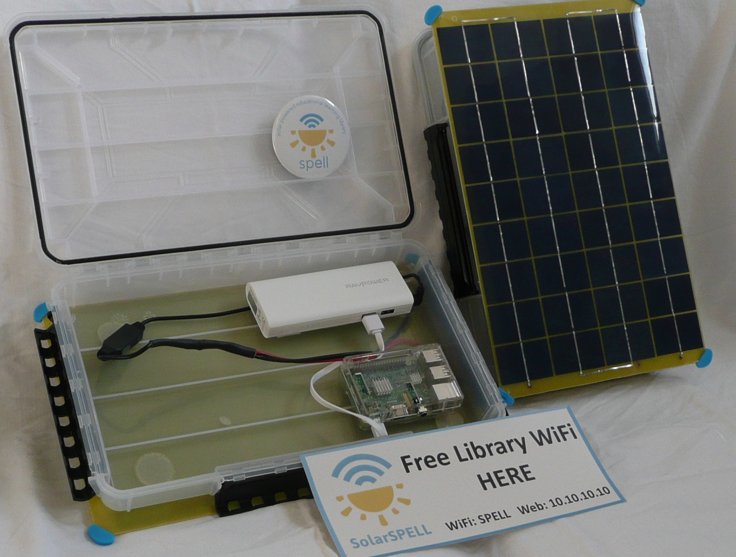 |
| A solar-powered, offline digital library. |
Aside from the information sessions, students will also gain hands-on experience working in teams and problem solving for real-world topics. The SolarSPELL team will present the students with three different challenges for student teams to develop a proposed solution using machine learning. Students will then be eligible to apply for paid summer fellowship positions with SolarSPELL to develop and integrate one of the proposed machine learning models into SolarSPELL’s technology.
SolarSPELL is a student-driven initiative, so the solutions that the exploreCSR students develop will be implemented in our digital libraries to improve hundreds of library users’ experiences around the world. With libraries in 10 countries in the Pacific Islands and East Africa, and plans to expand to Latin America and the Middle East, these students will have a far-reaching impact.
Daehan Kwak, Kean University
My colleague Xudong Zhang and I created an undergraduate research study group centered on computer vision, with projects underway on student attention detection, mask and social distancing detection, and pill recognition for healthcare scenarios. As one example, a student created a pill detection application using data from the National Library of Medicine pillbox. This can be used, for example, by high-volume distribution pharmacies to be more efficient and accurate, or by retirement homes to verify the pills a resident is taking. We’re pleased to share that the pill recognition project won third place in the Kean Business Plan Competition and was accepted to be presented at Posters on the Hill 2022.
Matthew Roberts, Macquarie University
The School of Computing at Macquarie University is working to lower the barrier to entry for students who are new to experimenting with ML by employing real-world examples. This month, around fifty students will spend the week testing their ideas for solving autonomous aquatic vehicles challenges (for example, navigation) under guidance from Macquarie University researchers. They will be developing their ideas with a sophisticated simulation environment, and the best solutions will be ready for deployment to real hardware testing in the water later in the year.
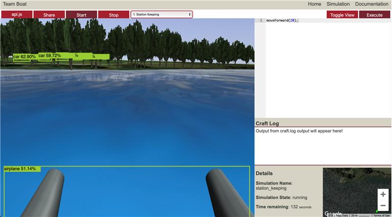 |
| A MacSim simulation of the Sydney Regatta Center (created by VRX), a placeholder for a machine learning model, is making random predictions, ready for improvements the students come up with. |
Accurately simulated sensors like cameras and LIDAR can be subjected to various models, allowing people to experiment with even more sophisticated ideas to solve complex problems. After our first year in exploreCSR, the adjustments we made to our simulator and the workshop will generate new ideas and light a spark for machine learning research early in students’ careers.
Pooyan Fazli, San Francisco State University
60+ students from 10 universities and colleges attended our 2-day virtual exploreCSR workshop. Participants were from San Francisco State University, CSU East Bay, CSU San Marcos, CSU Stanislaus, Foothill College, Northwestern University, San Diego State University, Sonoma State University, UC San Diego, and the University of San Francisco.
We had two invited speakers and two panels on mentorship and career pathways with 10 panelists from Google Research, Stanford, Emory University, Virginia Tech, and the University of Copenhagen.
As part of this workshop, we organized hands-on activities to introduce students to different aspects of AI and its applications for social good, such as with climate change. We also had mini-presentations and discussions on AI fairness, accountability, transparency and ethics in different areas, such as robotics, educational data mining, and impacts on underserved communities.
Following the workshop, selected students will participate in a research project under the guidance of graduate students and faculty during the spring semester. Through the research projects, we have a two-fold aim: to help students develop a sense of belonging in the AI and machine learning research community, and to illuminate a pathway for them to pursue graduate studies in AI/ML that explores the potential of developing responsible AI toward social good.
The research projects will begin with eight weekly meetups and hands-on training on Python programming with open-source publicly available materials. Then, students will engage in applied research projects that focus on AI applications for social good, such as health, environment, safety, education, climate change, and accessibility.
Farzana Rahman, Syracuse University
Earlier this year, the Electrical Engineering and Computer Science department of Syracuse University hosted RESORC (REsearch Exposure in Socially Relevant Computing), an exploreCSR program, for the second time. This program provided research exposure to 78 undergraduate students from SU and nearby institutions targeting populations historically underrepresented in computing. The goal of these two workshops was to give students an opportunity to learn machine learning using open-source tools, and to gain experience with data science workflows including collecting and labeling data, training a model, and carefully evaluating it. The ML workshops were the mostly highly rated sessions of the RESORC program.
Erin Hestir and Leigh Bernacchi, University of California, Merced
Since 2019, University of California, Merced has partnered with Merced College and California State University Stanislaus on the Google exploreCSR program ¡Valle! Get Your Start in Tech!, serving 32 Central Valley of California undergraduates in STEM annually to build a sense of belonging, practice professional networking, and develop technical skills. Participants convene on Zoom and in-person this semester. Valle students typically come from historically underrepresented groups, and the program is designed to support their pursuits of computational research, graduate school and computer science related careers. Many have gone on to achieve just that!
This year we added additional training thanks to Google Research to support machine learning applications for social good. This program is open to all Valle participants as well as partner schools, inclusive of graduate and undergraduate students in all STEM fields, and will be taught by creative graduate students in computer science from UC Merced. Each workshop will be taught by a near-peer mentor—a practice that supports mutual success in academics—and the mentor will coach teams to develop ML projects for social good.
The goal of the program is to overcome some of the trepidation scientists and students may have about computational science and machine learning through teamwork, fun and a higher purpose. Students will be able to develop their skills and interest, focusing on ML applications to climate, sustainability, agriculture and food, and diversity in tech and aviation.
Basak Guler, University of California, Riverside
At the University of California, Riverside, we created an undergraduate research study group focused on federated and distributed machine learning. Federated learning has become widely popular in recent years due to its communication efficiency and on-device learning architecture. Our study group meets on a weekly basis, and students learn about the principles of federated and distributed learning, state-of-the-art federated learning algorithms, recent applications from financial services to healthcare, as well as recent challenges and advances in privacy, security, and fairness. Student projects provide opportunities for undergraduate students to be involved in machine learning research, and learn from the experiences of both faculty and graduate students. This program can facilitate their transition from undergraduate to graduate degrees, and prepare them for positions of leadership in industry, government, public service, and academia.
Gonzalo A. Bello, University of Illinois at Chicago
The computer science department is hosting a series of exploreCSR workshops, including exploreCSR: Exploring Data Science Research, to introduce students to data science and machine learning research. These workshops aim to encourage students from historically underrepresented groups to pursue graduate studies and careers in research in the field of computer science. UIC students from all majors were encouraged to apply, including those who haven’t taken any computer science courses. Each semester, 60 students were selected out of more than 120 who applied, and 10 teaching assistants and a professor mentored students. In addition to lectures, students work on hands-on projects together where they explore, visualize, and build models using real-world data from the city of Chicago.
 |
Melanie Moses and Humayra Tasnim, The University of New Mexico
The UNM Google exploreCSR activity for 2021-2022 is a semester-long course called Swarmathon: The Next Generation. The students will learn technical skills like developing machine learning models for object recognition in robots, and soft skills including team building, research skills, and discussions with faculty and external speakers. The UNM exploreCSR program builds on 5 years of training students in a NASA-sponsored robotics competition called the Swarmathon (2014-2019). In 2019/2020 we developed a series of exploreCSR Swarmathon: TNG workshops which included a faculty panel, an industry mentor, an open-source tutorial, and a day-long workshop to enable “Swarmie” robots to classify and automatically retrieve objects.
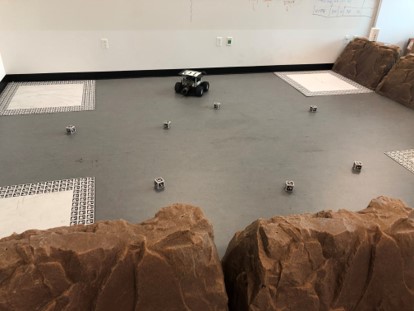 |
| A glimpse of our robots in action. |
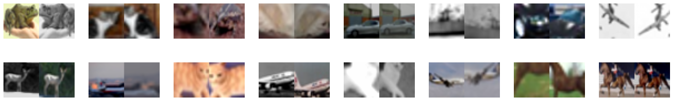
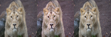
This year, in our exploreCSR Swarmathon: TNG course, students will have additional time to actively engage in developing and tuning their own machine learning models to test in the Swarmie robots. They will develop object detection models using convolutional neural networks (CNNs). They will be provided with a dataset of images of objects (shown below) taken from the robot camera and a simple model. The students will further develop the model and training data and then test their models on actual robots in real-time to see how much they can improve object recognition models to classify and retrieve the proper specified objects.
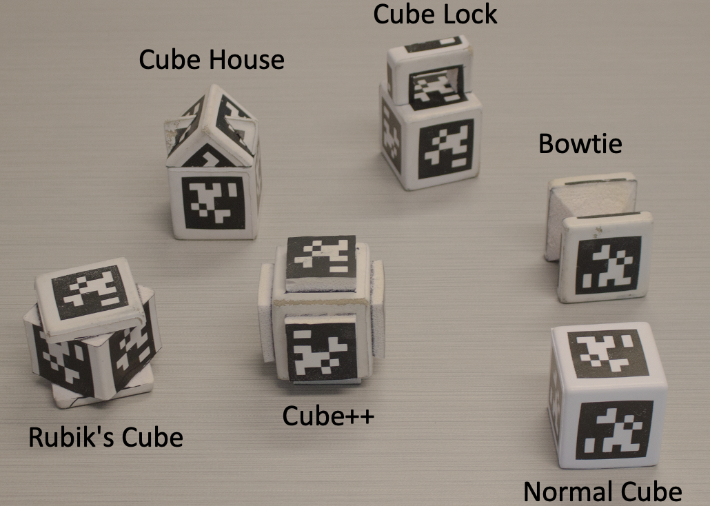 |
| Different shaped cubes for detection. |
Students will learn first-hand the reality gap between simulations and real-world experiments. This will encourage them to develop their own mini-research projects to enhance their model performance to resolve that gap. The exploreCSR-funded Swarmathon: TNG course will provide students with the opportunity to actively engage in hands-on robotics research. We hope the experience of defining a research objective, conducting a set of experiments, testing a model, and seeing results play out in our robotics arena will motivate students to attend graduate school and consider research careers.
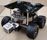 |
| Swarmie with a cube in its gripper. |
Daniel Mejía, The University of Texas at El Paso
We’re building a series of workshops open to undergraduate students of all majors to introduce them to applied machine learning and research topics, starting with foundational concepts in math and a newfound way of approaching a problem through the eyes of a data scientist. These workshops are open to all students, including those who do not have any prior experience. We hope to encourage students to consider pursuing graduate studies, especially those who may have not previously considered it. I believe that the earlier students are exposed, the more likely that they will pursue a graduate degree.
Henry Griffith, The University of Texas at San Antonio
At the University of Texas at San Antonio, we’re creating a portfolio of programs to enhance the persistence of first year Electrical and Computer Engineering students into research computing pathways. By integrating our programming with our Introduction to Electrical and Computer Engineering course, which has a total annual enrollment of approximately 200 students, we have the opportunity to achieve tremendous scale with our efforts. Our programs include an undergraduate research experience, a near-peer mentoring program, and group study projects – all designed to develop students’ professional and technical skills and to accelerate their progression into research opportunities.
John Akers, University of Washington
Our exploreCSR workshop, CSNext, is scheduled to begin this April. It’s a 4-week online program of workshops, seminars, and project work designed to encourage undergraduate students – particularly those from historically underrepresented groups – to consider and successfully apply to graduate schools in computer science. Participants will hear presentations from several University of Washington labs, such as Computer Vision/Graphics (GRAIL), Security and Privacy, and Human-Computer Interaction. There will be presentations on deep learning and on current graduate-level research, a panel discussion from current UW CSE grad students from varying backgrounds, opportunities to meet current graduate students from several UW CSE labs, and participants will be led through small-group exercises learning about active research from graduate student mentors. Participants will also learn about graduate school application processes and resources, led by staff from UW CSE Graduate Student Services.
Learning more
If you’re interested in creating your own programs like these with support from Google, keep an eye on the exploreCSR website for the next round of applications opening in June 2022.


