Posts in category: Tensorflow

A guest post by Charles Gaillard, Mindee

Introduction

Optical Character Recognition (OCR) refers to technologies capable of capturing text elements from images or documents and converting them into a machine-readable text format. If you want to learn more on that topic, this article is a good introduction.

At Mindee, we have developed an open-source Python-based OCR called DocTR, however we also wanted to deploy it in the browser to ensure that it was accessible to all developers – especially as ~70% developers choose to use JavaScript.

We managed to achieve this using the TensorFlow.js API, which resulted in a web demo that you can now try for yourself using images of your own.

The demo interface with a picture of 2 receipts being parsed by the OCR: 89 words were found here

This demo is designed to be very simple to use and run quickly on most computers, therefore we provided a single pretrained model that we trained with a small (512 x 512) input size to save memory. Images are resized to be squares, so it generalizes well to most of the documents which have an aspect ratio close to 1: cards, smaller receipts, tickets, A4, etc. For rectangles with a very high aspect ratio, segmentation results might not be as good because we don’t preserve the aspect ratio (with padding) at the text detection step. It is optimized to work on documents with a significant word size (for example receipts, cards, etc). Keep in mind that these models have been designed to offer performance while running in the browser. Hence, performance might not be optimal on documents that have a very small writing size vs the size of the document or images with a very high aspect ratio.

Dive into the architecture

OCR models can be divided into 2 parts: A detection model and a text recognition model. In DocTR, the detection model is a CNN (convolutional neural network) which segments the input image to find text areas, then text boxes are cropped around each detected word and sent to a recognition model. The second model is a convolutional recurrent neural network (CRNN), which extracts features from word-images and then decodes the sequence of letters on the image with recurrent layers (LSTM).

Global architecture of the OCR model used in this Demo

Detection model

We have different architectures implemented in DocTR, but we chose a very light one for use on the client side as device hardware can change from person to person. Here we used a mobilenetV2 backbone with a DB (Differentiable Binarization) head. The implementation details can be found in the DocTR Github. We trained this model with an input size of (512, 512, 3) to decrease latency and memory usage. We have a private dataset composed of 130,000 annotated documents that was used to train this model.

Recognition model

The recognition model we used is also our lighter architecture: a CRNN (convolutional recurrent neural network) with a mobilenetV2 backbone. More information on this architecture can be found here. It is basically composed of the first half of the mobilenetV2 layers to extract features and it is followed by 2 bi-LSTMs to decode visual features as character sequences (words). It uses the CTC loss, introduced by Alex Graves, to decode a sequence efficiently. We have an input size of (32, 128, 3) for word images in this model, and we use padding to preserve the aspect ratio of crops. It is trained on our private dataset, composed of 11 millions text boxes extracted from different documents. This dataset has a wide variety of fonts, since it is composed of documents which come from many different data sources. We used data augmentation so that it generalizes well on different fonts, backgrounds, and renderings. It should also give decent results on handwritten text as long as it is human-readable.

Model conversion & code implementation

As our model was originally implemented using TensorFlow, Python conversion was required to run the resulting models in the web browser at scale. To do this we exported a tensorflow SavedModel for each Python model trained and used the tensorflowjs_converter command line tool to quickly convert our saved models to the TensorFlow.js JSON format required for execution in the browser.

The resulting converted models were then integrated into our React.js front end application that powered the user interface of the demo. More precisely, we used MUI to design the components of the interface for our in-house front-end SDK react-mindee-js (which provides computer vision tools) and OpenCV.js for the detection model post processing. This post processing step took the raw binarized segmentation map and converted it to a list of polygons with OpenCV.js functions. We could then crop those boxes from the source image to finally obtain word images ready to be sent to the recognition model.

Speed & performance

We had to manage the tradeoff between speed and performance efficiently. OCR models are quite slow because you have 2 tasks (text areas segmentation + words recognition) that can’t be parallelized, so we had to use lightweight models to ensure speedy execution on most devices.

On an modern computer with an RTX 2060 and an i7 9th Gen, the detection task takes around 750 milliseconds per image, and the recognition model around 170 milliseconds per batch of 32 crops (words) with the WebGL backend, benchmarked with the TensorFlow.js benchmarking tool.

Wrapping up the 2 models and the vision operations (detection post processing), the end-to-end OCR runs in less than 2 seconds on small documents (less than 100 words) and the prediction time can only take a few seconds more to run on very dense documents with a lot of words.

A screenshot of the demo interface with a very dense old A4 document being parsed by the OCR: 738 words are identified.

Conclusion

This demo powered by TensorFlow.js is a way to give access to an online, relatively quick and robust document OCR to almost everyone, which is one of the first of its kind powered by TensorFlow.js entirely in the browser.

As we are executing the model on the client side, exact performance will vary depending on the hardware of the device it is run on. However the goal here is more to demonstrate that even complex and state-of-the-art deep learning models can be deployed in the browser and run on almost every machine in an efficient manner that can be very useful, especially for potentially sensitive document information, where you do not want to send the document to the cloud for analysis.

We are excited to offer this solution for all to use, and keen to follow the future of the Web ML industry, where things will no doubt get faster with time as new web standards like WebGPU become mainstream and enabled by default on modern web browsers.

Read More

Posted by Nikita Namjoshi, Google Cloud Developer Advocate

When you start working on a new machine learning problem, I’m guessing the first environment you use is a notebook. Maybe you like running Jupyter in a local environment, using a Kaggle Kernel, or my personal favorite, Colab. With tools like these, creating and experimenting with machine learning is becoming increasingly accessible. But while experimentation in notebooks is great, it’s easy to hit a wall when it comes time to elevate your experiments up to production scale. Suddenly, your concerns are more than just getting the highest accuracy score.

What if you have a long running job, want to do distributed training, or host a model for online predictions? Or maybe your use case requires more granular permissions around security and data privacy. What is your data going to look like at serving time, how will you handle code changes, or monitor the performance of your model overtime?

Making production applications or training large models requires additional tooling to help you scale beyond just code in a notebook, and using a cloud service provider can help. But that process can feel a bit daunting. Take a look at the full list of Google Cloud products, and you might be completely unsure where to start.

So to make your journey a little easier, I’ll show you a fast path from experimental notebook code to a deployed model in the cloud.

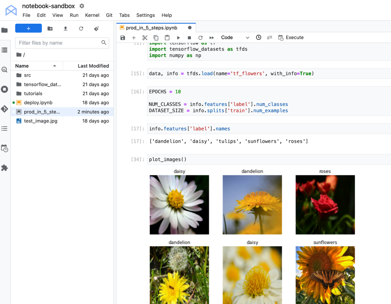
The code used in this sample can be found here. This notebook trains an image classification model on the TF Flowers dataset. You’ll see how to deploy this model in the cloud and get predictions on a new flower image via a REST endpoint.

Note that you’ll need a Google Cloud project with billing enabled to follow this tutorial. If you’ve never used Google Cloud before, you can follow these instructions to set up a project and get $300 in free credits to experiment with.

Here are the five steps you’ll take:

1. Create a Vertex AI Workbench managed notebook
2. Upload .ipynb file
3. Launch notebook execution
4. Deploy model
5. Get predictions

Create a Vertex AI Workbench managed notebook

To train and deploy the model, you’ll use Vertex AI, which is Google Cloud’s managed machine learning platform. Vertex AI contains lots of different products that help you across the entire lifecycle of an ML workflow. You’ll use a few of these products today, starting with Workbench, which is the managed notebook offering.

Under the Vertex AI section of the cloud console, select “Workbench”. Note that if this is the first time you’re using Vertex AI in a project, you’ll be prompted to enable the Vertex API and the Notebooks API. So be sure to click the button in the UI to do so.

Next, select MANAGED NOTEBOOKS, and then NEW NOTEBOOK.

Under Advanced Settings you can customize your notebook by specifying the machine type and location, adding GPUs, providing custom containers, and enabling terminal access. For now, keep the default settings and just provide a name for your notebook. Then click CREATE.

You’ll know your notebook is ready when you see the OPEN JUPYTERLAB text turn blue. The first time you open the notebook, you’ll be prompted to authenticate and you can follow the steps in the UI to do so.

When you open the JupyterLab instance, you’ll see a few different notebook options. Vertex AI Workbench provides different kernels (TensorFlow, R, XGBoost, etc), which are managed environments preinstalled with common libraries for data science. If you need to add additional libraries to a kernel, you can use pip install from a notebook cell, just like you would in Colab.

Step one is complete! You’ve created your managed JupyterLab environment.

Upload .ipynb file

Now it’s time to get our TensorFlow code into Google Cloud. If you’ve been working in a different environment (Colab, local, etc), you can upload any code artifacts you need to your Vertex AI Workbench managed notebook, and you can even integrate with GitHub. In the future, you can do all of your development right in Workbench, but for now let’s assume you’ve been using Colab.

Colab notebooks can be exported as .ipynb files.

You can upload the file to Workbench by clicking the “upload files” icon.

When you open the notebook in Workbench, you’ll be prompted to select the kernel, which is the environment where your notebook is run. There are a few different kernels you can choose from, but since this code sample uses TensorFlow, you’ll want to select the TensorFlow 2 kernel.

After you select the kernel, any cells you execute in your notebook will run in this managed TensorFlow environment. For example, if you execute the import cell, you’ll see that you can import TensorFlow, TensorFlow Datasets, and NumPy. This is because all of these libraries are included in the Vertex AI Workbench TensorFlow 2 kernel. Unsurprisingly, if you try to execute that same notebook cell in the XGBoost kernel, you’ll see an error message since TensorFlow is not installed there.

Launch a notebook execution

While we could run the rest of the notebook cells manually, for models that take a long time to train, a notebook isn’t always the most convenient option. And if you’re building an application with ML, it’s unlikely that you’ll only need to train your model once. Over time, you’ll want to retrain your model to make sure it stays fresh and keeps producing valuable results.

Manually executing the cells of your notebook might be the right option when you’re getting started with a new machine learning problem. But when you want to automate experimentation at a large scale, or retrain models for a production application, a managed ML training option will make things much easier.

The quickest way to launch a training job is through the notebook execution feature, which will run the notebook cell by cell on the Vertex AI managed training service.

When you launch the training job, it’s going to run on a machine you won’t have access to after the job completes. So you don’t want to save the TensorFlow model artifacts to a local path. Instead, you’ll want to save to Cloud Storage, which is Google Cloud’s object storage, meaning you can store images, csv files, txt files, saved model artifacts. Just about anything.

Cloud storage has the concept of a “bucket” which is what holds your data. You can create them via the UI. Everything you store in Cloud Storage must be contained in a bucket. And within a bucket, you can create folders to organize your data.

Each file in Cloud Storage has a path, just like a file on your local filesystem. Except that Cloud Storage paths always start with gs://

You’ll want to update your training code so that you’re saving to a Cloud Storage bucket instead of a local path.

For example, here I’ve updated the last cell of the notebook from model.save('model_ouput").Instead of saving locally, I’m now saving the artifacts to a bucket called nikita-flower-demo-bucket that I’ve created in my project.

Now we’re ready to launch the execution.

Select the Execute button, give your execution a name, then add a GPU. Under Environment, select the TensorFlow 2.7 GPU image. This container comes preinstalled with TensorFlow and many other data science libraries.

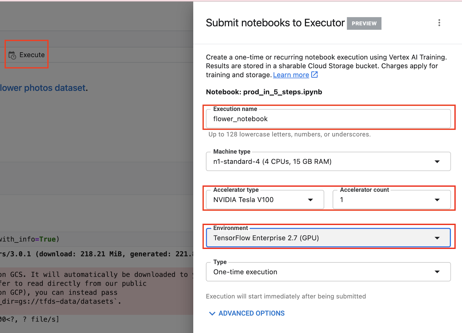
Then click SUBMIT.

You can track the status of your training job in the EXECUTIONS tab. The notebook and the output of each cell will be visible under VIEW RESULT when the job finishes and is stored in a GCS bucket. This means you can always tie a model run back to the code that was executed.

When the training completes you’ll be able to see the TensorFlow saved model artifacts in your bucket.

Deploy to endpoint

Now you know how to quickly launch serverless training jobs on Google Cloud. But ML is not just about training. What’s the point of all this effort if we don’t actually use the model to do something, right?

Just like with training, we could execute predictions directly from our notebook by calling model.predict. But when we want to get predictions for lots of data, or get low latency predictions on the fly, we’re going to need something more powerful than a notebook.

Back in your Vertex AI Workbench managed notebook, you can paste the code below in a cell, which will use the Vertex AI Python SDK to deploy the model you just trained to the Vertex AI Prediction service. Deploying the model to an endpoint associates the saved model artifacts with physical resources for low latency predictions.

First, import the Vertex AI Python SDK.

from google.cloud import aiplatform

Then, upload your model to the Vertex AI Model Registry. You’ll need to give your model a name, and provide a serving container image, which is the environment where your predictions will run. Vertex AI provides pre-built containers for serving, and in this example we’re using the TensorFlow 2.8 image.

You’ll also need to replace artifact_uri with the path to the bucket where you stored your saved model artifacts. For me, that was “nikita-flower-demo-bucket”. You’ll also need to replace project with your project ID.

my_model = aiplatform.Model.upload(display_name='flower-model',
                                  artifact_uri='gs://{YOUR_BUCKET}',
                                  serving_container_image_uri='us-docker.pkg.dev/vertex-ai/prediction/tf2-cpu.2-8:latest',
                                  project={YOUR_PROJECT})

Then deploy the model to an endpoint. I’m using default values for now, but if you’d like to learn more about traffic splitting, and autoscaling, be sure to check out the docs. Note that if your use case does not require low latency predictions, you don’t need to deploy the model to an endpoint and can use the batch prediction feature instead.

endpoint = my_model.deploy(
     deployed_model_display_name='my-endpoint',
     traffic_split={"0": 100},
     machine_type="n1-standard-4",
     accelerator_count=0,
     min_replica_count=1,
     max_replica_count=1,
   )

Once the deployment has completed, you can see your model and endpoint in the console

Get predictions

Now that this model is deployed to an endpoint, you can hit it like any other REST endpoint. This means you can integrate your model and get predictions into a downstream application.

For now, let’s just test it out directly within Workbench.

First, open a new TensorFlow notebook.

In the notebook, import the Vertex AI Python SDK.

from google.cloud import aiplatform

Then, create your endpoint, replacing project_number and endpoint_id.

endpoint = aiplatform.Endpoint(
    endpoint_name="projects/{project_number}/locations/us-central1/endpoints/{endpoint_id}")

You can find your endpoint_id in the Endpoints section of the cloud Console.

You can find your Project Number on the home page of the console. Note that this is different from the Project ID.

When you send a request to an online prediction server, the request is received by an HTTP server. The HTTP server extracts the prediction request from the HTTP request content body. The extracted prediction request is forwarded to the serving function. The basic format for online prediction is a list of data instances. These can be either plain lists of values or members of a JSON object, depending on how you configured your inputs in your training application.

To test the endpoint, I first uploaded an image of a flower to my workbench instance.

The code below opens and resizes the image with PIL, and converts it into a numpy array.

import numpy as np
from PIL import Image

IMAGE_PATH = 'test_image.jpg'

im = Image.open(IMAGE_PATH)
im = im.resize((150, 150))

Then, we convert our numpy data to type float32 and to a list. We convert to a list because numpy data is not JSON serializable so we can’t send it in the body of our request. Note that we don’t need to scale the data by 255 because that step was included as part of our model architecture using tf.keras.layers.Rescaling(1./255). To avoid having to resizing our image, we could have added tf.keras.layers.Resizing to our model, instead of making it part of the tf.data pipeline.

# convert to float32 list
x_test = [np.asarray(im).astype(np.float32).tolist()]

Then, we call call predict

endpoint.predict(instances=x_test).predictions

The result you get is the output of the model, which is a softmax layer with 5 units. Looks like class at index 2 (tulips) scored the highest.

[[0.0, 0.0, 1.0, 0.0, 0.0]]

Tip: to save costs, be sure to undeploy your endpoint if you’re not planning to use it! You can undeploy by going to the Endpoints section of the console, selecting the endpoint and then the Undeploy model form endpoint option. You can always redeploy in the future if needed.

For more realistic examples, you’ll probably want to directly send the image itself to the endpoint, instead of loading it in NumPy first. If you’d like to see an example, check out this notebook.

What’s Next

You now know how to get from notebook experimentation to deployment in the cloud. With this framework in mind, I hope you start thinking about how you can build new ML applications with notebooks and Vertex AI.

If you’re interested in learning even more about how to use Google Cloud to get your TensorFlow models into production, be sure to register for the upcoming Google Cloud Applied ML Summit. This virtual event is scheduled for 9th June and brings together the world’s leading professional machine learning engineers and data scientists. Connect with other ML engineers and data scientists and discover new ways to speed up experimentation, quickly get into production, scale and manage models, and automate pipelines to deliver impact. Reserve your seat today!

Read More

Posted by Hugo Zanini, Data Product Manager

Last year, I published an article on how to train custom object detection in the browser using TensorFlow.js. This received lots of interest from developers from all over the world who tried to apply the solution to their personal or business projects.While answering reader’s questions on my first article, I noticed a few difficulties in adapting our solution to large datasets, and deploying the resulting model in production using the new version of TensorFlow.js.

Therefore, the goal of this article is to share a solution for a well-known problem in the consumer packaged goods (CPG) industry: real-time and offline SKU detection using TensorFlow.js.

The problem

Items consumed frequently by consumers (foods, beverages, household products, etc) require an extensive routine of replenishment and placement of those products at their point of sale (supermarkets, convenience stores, etc).

Over the past few years, researchers have shown repeatedly that about two-thirds of purchase decisions are made after customers enter the store. One of the biggest challenges for consumer goods companies is to guarantee the availability and correct placement of their product in-stores.

At stores, teams organize the shelves based on marketing strategies, and manage the level of products in the stores. The people working on these activities may count the number of SKUs of each brand in a store to estimate product stocks and market share, and help to shape marketing strategies.

These estimations though are very time-consuming. Taking a photo and using an algorithm to count the SKUs on the shelves to calculate a brand’s market share could be a good solution.

To use an approach like that, the detection should run in real-time such that as soon as you point a phone camera to the shelf, the algorithm recognizes the brands and calculates the market shares. And, as the internet inside the stores is generally limited, the detection should work offline.

This post is going to show how to implement the real-time and offline image recognition solution to identify generic SKUs using the SKU110K dataset and the MobileNetV2 network.

Due to the lack of a public dataset with labeled SKUs of different brands, we’re going to create a generic algorithm, but all the instructions can be applied in a multiclass problem.

As with every machine learning flow, the project will be divided into four steps, as follows:

Preparing the data

The first step to training a good model is to gather good data. As mentioned before, this solution is going to use a dataset of SKUs in different scenarios. The purpose of SKU110K was to create a benchmark for models capable of recognizing objects in densely packed scenes.

The dataset is provided in the Pascal VOC format and has to be converted to tf.record. The script to do the conversion is available here and the tf.record version of the dataset is also available in my project repository. As mentioned before, SKU110K is a large and very challenging dataset to work with. It contains many objects, often looking similar or even identical, positioned in close proximity.

To work with this dataset, the neural network chosen has to be very effective in recognizing patterns and be small enough to run in real-time in TensorFlow.js.

Choosing the model

There are a variety of neural networks capable of solving the SKU detection problem. But, the architectures that easily achieve a high level of precision are very dense and don’t have reasonable inference times when converted to TensorFlow.js to run in real-time.

Because of that, the approach here is going to be to focus on optimizing a mid-level neural network to achieve reasonable precision working on densely packed scenes and run the inferences in real-time. Analyzing the TensorFlow 2.0 Detection Model Zoo, the challenge will be to try to solve the problem using the lighter single-shot model available: SSD MobileNet v2 320×320 which seems to fit the criteria required. The architecture is proven to be able to recognize up to 90 classes and can be trained to identify different SKUs.

Training the model

With a good dataset and the model selected, it’s time to think about the training process. TensorFlow 2.0 provides an Object Detection API that makes it easy to construct, train, and deploy object detection models. In this project, we’re going to use this API and train the model using a Google Colaboratory Notebook. The remainder of this section explains how to set up the environment, the model selection, and training. If you want to jump straight to the Colab Notebook, click here.

Setting up the environment

Create a new Google Colab notebook and select a GPU as the hardware accelerator:

Runtime > Change runtime type > Hardware accelerator: GPU

Clone, install, and test the TensorFlow Object Detection API:

Next, download and extract the dataset using the following commands:

Setting up the training pipeline

We’re ready to configure the training pipeline. TensorFlow 2.0 provides pre-trained weights for the SSD Mobilenet v2 320×320 on the COCO 2017 Dataset, and they are going to be downloaded using the following commands:

The downloaded weights were pre-trained on the COCO 2017 Dataset, but the focus here is to train the model to recognize one class so these weights are going to be used only to initialize the network — this technique is known as transfer learning, and it’s commonly used to speed up the learning process.

The last step is to set up the hyperparameters on the configuration file that is going to be used during the training. Choosing the best hyperparameters is a task that requires some experimentation and, consequently, computational resources.

I took a standard configuration of MobileNetV2 parameters from the TensorFlow Models Config Repository and performed a sequence of experiments (thanks Google Developers for the free resources) to optimize the model to work with densely packed scenes on the SKU110K dataset. Download the configuration and check the parameters using the code below.

With the parameters set, start the training by executing the following command:

To identify how well the training is going, we use the loss value. Loss is a number indicating how bad the model’s prediction was on the training samples. If the model’s prediction is perfect, the loss is zero; otherwise, the loss is greater. The goal of training a model is to find a set of weights and biases that have low loss, on average, across all examples (Descending into ML: Training and Loss | Machine Learning Crash Course).

The training process was monitored through Tensorboard and took around 22h to finish on a 60GB machine using an NVIDIA Tesla P4. The final losses can be checked below

Validate the model

Now let’s evaluate the trained model using the test data:

The evaluation was done across 2740 images and provides three metrics based on the COCO detection evaluation metrics: precision, recall, and loss (Classification: Precision and Recall | Machine Learning Crash Course). The same metrics are available via Tensorboard and can be analyzed in an easier way

%load_ext tensorboard
%tensorboard --logdir '/content/training/'

You can then explore all training and evaluation metrics.

Exporting the model

Now that the training is validated, it’s time to export the model. We’re going to convert the training checkpoints to a protobuf (pb) file. This file is going to have the graph definition and the weights of the model.

As we’re going to deploy the model using TensorFlow.js and Google Colab has a maximum lifetime limit of 12 hours, let’s download the trained weights and save them locally. When running the command files.download("/content/saved_model.zip"), the Colab will prompt the file download automatically.

Deploying the model

The model is going to be deployed in a way that anyone can open a PC or mobile camera and perform inference in real-time through a web browser. To do that, we’re going to convert the saved model to the TensorFlow.js layers format, load the model in a JavaScript application and make everything available on CodeSandbox.

Converting the model

At this point, you should have something similar to this structure saved locally:

%MD

├── inference-graph

│ ├── saved_model

│ │ ├── assets

│ │ ├── saved_model.pb

│ │ ├── variables

│ │ ├── variables.data-00000-of-00001

│ │ └── variables.index

Before we start, let’s create an isolated Python environment to work in an empty workspace and avoid any library conflict. Install virtualenv and then open a terminal in the inference-graph folder and create and activate a new virtual environment:

virtualenv -p python3 venv
source venv/bin/activate

Install the TensorFlow.js converter:

pip install tensorflowjs[wizard]

Start the conversion wizard:

tensorflowjs_wizard

Now, the tool will guide you through the conversion, providing explanations for each choice you need to make. The image below shows all the choices that were made to convert the model. Most of them are the standard ones, but options like the shard sizes and compression can be changed according to your needs.

To enable the browser to cache the weights automatically, it’s recommended to split them into shard files of around 4MB. To guarantee that the conversion is going to work, don’t skip the op validation as well, not all TensorFlow operations are supported so some models can be incompatible with TensorFlow.js — See this list for which ops are currently supported on the various backends that TensorFlow.js executes on such as WebGL, WebAssembly, or plain JavaScript.

If everything works well, you’re going to have the model converted to the TensorFlow.js layers format in the web_model directory. The folder contains a model.json file and a set of sharded weights files in a binary format. The model.json has both the model topology (aka “architecture” or “graph”: a description of the layers and how they are connected) and a manifest of the weight files (Lin, Tsung-Yi, et al). The contents of the web_model folder currently contains the files shown below:

└ web_model
  ├── group1-shard1of5.bin
  ├── group1-shard2of5.bin
  ├── group1-shard3of5.bin
  ├── group1-shard4of5.bin
  ├── group1-shard5of5.bin
  └── model.json

Configuring the application

The model is ready to be loaded in JavaScript. I’ve created an application to perform inference directly from the browser. Let’s clone the repository to figure out how to use the converted model in real-time. This is the project structure:

├── models
│	├── group1-shard1of5.bin
│	├── group1-shard2of5.bin
│	├── group1-shard3of5.bin
│	├── group1-shard4of5.bin
│	├── group1-shard5of5.bin
│	└── model.json
├── package.json
├── package-lock.json
├── public
│   └── index.html
├── README.MD
└── src
	├── index.js
	└── styles.css

For the sake of simplicity, I have already provided a converted SKU-detector model in the model’s folder. However, let’s put the web_model generated in the previous section in the models folder and test it.

Next, install the http-server:

npm install http-server -g

Go to the models folder and run the command below to make the model available at http://127.0.0.1:8080 . This is a good choice when you want to keep the model weights in a safe place and control who can request inferences to it. The -c1 parameter is added to disable caching, and the –cors flag enables cross-origin resource sharing allowing the hosted files to be used by the client-side JavaScript for a given domain.

http-server -c1 --cors .

Alternatively, you can upload the model files somewhere else – even on a different domain if needed. In my case, I chose my own Github repo and referenced the model.json folder URL in the load_model function as shown below:

async function load_model() {
	// It's possible to load the model locally or from a repo.
	// Load from localhost locally:
      const model = await loadGraphModel("http://127.0.0.1:8080/model.json");
	// Or Load from another domain using a folder that contains model.json.
      // const model = await loadGraphModel("https://github.com/hugozanini/realtime-sku-detection/tree/web");
	return model;
}

This is a good option because it gives more flexibility to the application and makes it easier to run on public web servers.

Pick one of the methods to load the model files in the function load_model (lines 10–15 in the file src>index.js).

When loading the model, TensorFlow.js will perform the following requests:

GET /model.json
GET /group1-shard1of5.bin
GET /group1-shard2of5.bin
GET /group1-shard3of5.bin
GET /group1-shardo4f5.bin
GET /group1-shardo5f5.bin

Publishing in CodeSandbox

CodeSandbox is a simple tool for creating web apps where we can upload the code and make the application available for everyone on the web. By uploading the model files in a GitHub repo and referencing them in the load_model function, we can simply log into CodeSandbox, click on New project > Import from Github, and select the app repository.

Wait some minutes to install the packages and your app will be available at a public URL that you can share with others. Click on Show > In a new window and a tab will open with a live preview. Copy this URL and paste it in any web browser (PC or Mobile) and your object detection will be ready to run. A ready to use project can be found here as well if you prefer.

Conclusion

Besides the precision, an interesting part of these experiments is the inference time — everything runs in real-time in the browser via JavaScript. SKU detection models running in the browser, even offline, and using few computational resources is a must in many consumer packaged goods company applications, along with other industries too.

Enabling a Machine Learning solution to run on the client-side is a key step to guarantee that the models are being used effectively at the point of interaction with minimal latency and solve the problems when they happen: right in the user’s hand.

Deep learning should not be costly and should be used beyond just research, for real world use cases, which JavaScript is great for production deployments. I hope this article will serve as a basis for new projects involving Computer Vision, TensorFlow, and create an easier flow between Python and Javascript.

If you have any questions or suggestions you can reach me on Twitter.

Thanks for reading!

Acknowledgments

I’d like to thank the Google Developers Group, for providing all the computational resources for training the models, and the authors of the SKU 110K Dataset, for creating and open-sourcing the dataset used in this project.

Read More

Posted by Goldie Gadde and Douglas Yarrington for the TensorFlow team

TensorFlow 2.9 has been released! Highlights include performance improvements with oneDNN, and the release of DTensor, a new API for model distribution that can be used to seamlessly move from data parallelism to model parallelism

We’ve also made improvements to the core library, including Eigen and tf.function unification, deterministic behavior, and new support for Windows’ WSL2. Finally, we’re releasing new experimental APIs for tf.function retracing and Keras Optimizers. Let’s take a look at these new and improved features.

Improved CPU performance: oneDNN by default

We have worked with Intel to integrate the oneDNN performance library with TensorFlow to achieve top performance on Intel CPUs. Since TensorFlow 2.5, TensorFlow has had experimental support for oneDNN, which could provide up to a 4x performance improvement. In TensorFlow 2.9, we are turning on oneDNN optimizations by default on Linux x86 packages and for CPUs with neural-network-focused hardware features such as AVX512_VNNI, AVX512_BF16, AMX, and others, which are found on Intel Cascade Lake and newer CPUs.

Users running TensorFlow with oneDNN optimizations enabled might observe slightly different numerical results from when the optimizations are off. This is because floating-point round-off approaches and order differ, and can create slight errors. If this causes issues for you, turn the optimizations off by setting TF_ENABLE_ONEDNN_OPTS=0 before running your TensorFlow programs. To enable or re-enable them, set TF_ENABLE_ONEDNN_OPTS=1 before running your TensorFlow program. To verify that the optimizations are on, look for a message beginning with "oneDNN custom operations are on" in your program log. We welcome feedback on GitHub and the TensorFlow Forum.

Model parallelism with DTensor

DTensor is a new TensorFlow API for distributed model processing that allows models to seamlessly move from data parallelism to single program multiple data (SPMD) based model parallelism, including spatial partitioning. This means you have tools to easily train models where the model weights or inputs are so large they don’t fit on a single device. (If you are familiar with Mesh TensorFlow in TF1, DTensor serves a similar purpose.)

DTensor is designed with the following principles at its core:

• A device-agnostic API: This allows the same model code to be used on CPU, GPU, or TPU, including models partitioned across device types.
• Multi-client execution: Removes the coordinator and leaves each task to drive its locally attached devices, allowing scaling a model with no impact to startup time.
• A global perspective vs. per-replica: Traditionally with TensorFlow, distributed model code is written around replicas, but with DTensor, model code is written from the global perspective and per replica code is generated and run by the DTensor runtime. Among other things, this means no uncertainty about whether batch normalization is happening at the global level or the per replica level.

We have developed several introductory tutorials on DTensor, from DTensor concepts to training DTensor ML models with Keras:

• DTensor Concepts
• Distributed ML with DTensors
• Using DTensors with Keras

TraceType for tf.function

We have revamped the way tf.function retraces to make it simpler, predictable, and configurable.

All arguments of tf.function are assigned a tf.types.experimental.TraceType. Custom user classes can declare a TraceType using the Tracing Protocol (tf.types.experimental.SupportsTracingProtocol).

The TraceType system makes it easy to understand retracing rules. For example, subtyping rules indicate what type of arguments can be used with particular function traces. Subtyping also explains how different specific shapes are joined into a generic shape that is their supertype, to reduce the number of traces for a function.

To learn more, see the new APIs for tf.types.experimental.TraceType, tf.types.experimental.SupportsTracingProtocol, and the reduce_retracing parameter of tf.function.

Support for WSL2

The Windows Subsystem for Linux lets developers run a Linux environment directly on Windows, without the overhead of a traditional virtual machine or dual boot setup. TensorFlow now supports WSL2 out of the box, including GPU acceleration. Please see the documentation for more details about the requirements and how to install WSL2 on Windows.

Deterministic behavior

The API tf.config.experimental.enable_op_determinism makes TensorFlow ops deterministic.

Determinism means that if you run an op multiple times with the same inputs, the op returns the exact same outputs every time. This is useful for debugging models, and if you train your model from scratch several times with determinism, your model weights will be the same every time. Normally, many ops are non-deterministic due to the use of threads within ops which can add floating-point numbers in a nondeterministic order.

TensorFlow 2.8 introduced an API to make ops deterministic, and TensorFlow 2.9 improved determinism performance in tf.data in some cases. If you want your TensorFlow models to run deterministically, just add the following to the start of your program:

“`

tf.keras.utils.set_random_seed(1)

tf.config.experimental.enable_op_determinism()

“`

The first line sets the random seed for Python, NumPy, and TensorFlow, which is necessary for determinism. The second line makes each TensorFlow op deterministic. Note that determinism in general comes at the expense of lower performance and so your model may run slower when op determinism is enabled.

Optimized Training with Keras

In TensorFlow 2.9, we are releasing a new experimental version of the Keras Optimizer API, tf.keras.optimizers.experimental. The API provides a more unified and expanded catalog of built-in optimizers which can be more easily customized and extended.

In a future release, tf.keras.optimizers.experimental.Optimizer (and subclasses) will replace tf.keras.optimizers.Optimizer (and subclasses), which means that workflows using the legacy Keras optimizer will automatically switch to the new optimizer. The current (legacy) tf.keras.optimizers.* API will still be accessible via tf.keras.optimizers.legacy.*, such as tf.keras.optimizers.legacy.Adam.

Here are some highlights of the new optimizer class:

• Incrementally faster training for some models.
• Easier to write customized optimizers.
• Built-in support for moving average of model weights (“Polyak averaging”).

For most users, you will need to take no action. But, if you have an advanced workflow falling into the following cases, please make corresponding changes:

Use Case 1: You implement a customized optimizer based on the Keras optimizer

For these works, please first check if it is possible to change your dependency to tf.keras.optimizers.experimental.Optimizer. If for any reason you decide to stay with the old optimizer (we discourage it), then you can change your optimizer to tf.keras.optimizers.legacy.Optimizer to avoid being automatically switched to the new optimizer in a later TensorFlow version.

Use Case 2: Your work depends on third-party Keras-based optimizers (such as tensorflow_addons)

Your work should run successfully as long as the library continues to support the specific optimizer. However, if the library maintainers fail to take actions to accommodate the Keras optimizer change, your work would error out. So please stay tuned with the third-party library’s announcement, and file a bug to Keras team if your work is broken due to optimizer malfunction.

Use Case 3: Your work is based on TF1

First of all, please try migrating to TF2. It is worth it, and may be easier than you think! If for any reason migration is not going to happen soon, then please replace your tf.keras.optimizers.XXX to tf.keras.optimizers.legacy.XXX to avoid being automatically switched to the new optimizer.

Use Case 4: Your work has customized gradient aggregation logic

Usually this means you are doing gradients aggregation outside the optimizer, and calling apply_gradients() with experimental_aggregate_gradients=False. We changed the argument name, so please change your optimizer to tf.keras.optimizers.experimental.Optimizer and set skip_gradients_aggregation=True. If it errors out after making this change, please file a bug to Keras team.

Use Case 5: Your work has direct calls to deprecated optimizer public APIs

Please check if your method call has a match here. change your optimizer to tf.keras.optimizers.experimental.Optimizer. If for any reason you want to keep using the old optimizer, change your optimizer to tf.keras.optimizers.legacy.Optimizer.

Next steps

Check out the release notes for more information. To stay up to date, you can read the TensorFlow blog, follow twitter.com/tensorflow, or subscribe to youtube.com/tensorflow. If you’ve built something you’d like to share, please submit it for our Community Spotlight at goo.gle/TFCS. For feedback, please file an issue on GitHub or post to the TensorFlow Forum. Thank you!

Read More

Posted by Scott Main, AIY Projects and Coral

Back in 2017, we began AIY Projects to make do-it-yourself artificial intelligence projects accessible to anybody. Our first project was the AIY Voice Kit, which allows you to build your own intelligent device that responds to voice commands. Then we released the AIY Vision Kit, which can recognize objects seen by its camera using on-device TensorFlow models. We were amazed by the projects people built with these kits and thrilled to see educational programs use them to introduce young engineers to the possibilities of computer science and machine learning (ML). So I’m excited to continue our mission to bring machine learning to everyone with the more powerful and more customizable AIY Maker Kit.

Making ML accessible to all

The Voice Kit and Vision Kit are a lot of fun to put together and they include great programs that demonstrate the possibilities of ML on a small device. However, they don’t provide the tools or procedures to help beginners achieve their own ML project ideas. When we released those kits in 2017, it was actually quite difficult to train an ML model, and getting a model to run on a device like a Raspberry Pi was even more challenging. Nowadays, if you have some experience with ML and know where to look for help, it’s not so surprising that you can train an object detection model in your web browser in less than an hour, or that you can run a pose detection model on a battery-powered device. But if you don’t have any experience, it can be difficult to discover the latest ML tools, let alone get started with them.

We intend to solve that with the Maker Kit. With this kit, we’re not offering any new hardware or ML tools; we’re offering a simplified workflow and a series of tutorials that use the latest tools to train TensorFlow Lite models and execute them on small devices. So it’s all existing technology, but better packaged so beginners can stop searching and start building incredible things right away.

Simplified tools for success

The material we’ve collected and created for the Maker Kit offers an end-to-end experience that’s ideal for educational programs and users who just want to make something with ML as fast as possible.

The hardware setup requires a Raspberry Pi, a Pi Camera, a USB microphone, and a Coral USB Accelerator so you can execute advanced vision models at high speed on the Coral Edge TPU. If you want your hardware in a case, we offer two DIY options: a 3D-printed case design or a cardboard case you can build using materials at home.

Once it’s booted up with our Maker Kit system image, just run some of our code examples and follow our coding tutorials. You’ll quickly discover how easy it is to accomplish amazing things with ML that were recently considered accessible only to experts, including object detection, pose classification, and speech recognition.

Our code examples use some pre-trained models and you can get more models that are accelerated on the Edge TPU from the Coral models library. However, training your own models allows you to explore all new project ideas. So the Maker Kit also offers step-by-step tutorials that show you how to collect your own datasets and train your own vision and audio models.

Last but not least, we want you to spend nearly all your time writing the code that’s unique to your project. So we created a Python library that reduces the amount of code needed to perform an inference down to a tiny part of your project. For example, this is how you can run an object detection model and draw labeled bounding boxes on a live camera feed:

from aiymakerkit import vision
from aiymakerkit import utils
import models

detector = vision.Detector(models.OBJECT_DETECTION_MODEL)
labels = utils.read_labels_from_metadata(models.OBJECT_DETECTION_MODEL)

for frame in vision.get_frames():
    objects = detector.get_objects(frame, threshold=0.4)
    vision.draw_objects(frame, objects, labels)

Our intent is to hide the code you don’t absolutely need. You still have access to structured inference results and program flow, but without any boilerplate code to handle the model.

This aiymakerkit library is built upon TensorFlow Lite and it’s available on GitHub, so we invite you to explore the innards and extend the Maker Kit API for your projects.

Getting started

We created the Maker Kit to be fully customizable for your projects. So rather than provide all the materials in a box with a predetermined design, we designed it with hardware that’s already available in stores (listed on our website) and with optional instructions to build your own case.

To get started, visit our website at g.co/aiy/maker, gather the required materials, flash our system image, and follow our programming tutorials to start exploring the possibilities. With this head start toward building smart applications that run entirely on an embedded system, we can’t wait to see what you will create.

Read More

Posted by TensorFlow Team

Google I/O 2022 was a major milestone in the evolution of AI and Machine Learning for developers. We’re really excited about the potential for developers using our technologies and Machine Learning to build intelligent solutions, and we believe that 2022 is the year when AI and ML become part of every developer’s toolbox.

At the I/O keynotes we showed our fully open source ecosystem that takes you from end to end with Machine Learning. There are developer tools for managing data, training your models, and deploying them to a variety of surfaces from global scale cloud all the way down to tiny microcontrollers…and of course ways to monitor and maintain your systems with MLOps. All of this comes with a common set of accelerated hardware for training and inference, along with open source tooling for responsible AI end-to-end.

You can get a tour through this ecosystem in the Keynote “AI and Machine Learning updates for Developers”

Responsible AI review processes: From a developer’s point of view

We can all agree that responsible and ethical AI is important, but when you want to build responsibly, you need tooling. We could, and will, create a whole video series about these tools, but the great content to watch right now is the talk on the Responsible AI review process. Googlers who worked on projects like the Covid-19 public forecasts or the Celebrity Recognition APIs will take you step-by-step through their thought process and how the tools lined up to help them build more responsibly and thoughtfully. You’ll also learn about some of the new releases in Responsible AI tools, such as the Counterfactual Logit Pairing library.

Adding machine learning to your developer toolbox

If you’re just getting started on your journey and you want ML to be a part of your toolbox, you probably have a million questions. Follow a developer’s journey through the best offerings, from a turnkey API that can solve basic problems fast, to custom models that can be tuned and deployed.

TensorFlow.js: From prototype to production, what’s new in 2022?

If you’re a web developer there’s a whole bunch of new updates, from the announcement of a new set of courses that will take you from first principles through a deep dive of what’s possible to lots of new models available to web devs. These include a selfie depth estimation model that can be used for cool things like a 3D effect in your pictures without needing any kind of extra sensor. You’ll also see 3D pose estimation that allows you to run at a high FPS to get real time results, allowing you to do things like having a full animated character following your body motion. All in the browser!

Deploy a custom ML model to mobile

If you want to build better mobile apps with AI and Machine Learning, you probably need to understand the ins and outs of getting models to execute on Android or iOS devices, including shrinking them and optimizing them to be power friendly. Supercharge your model with new releases from the TensorFlow Lite team that let you quantize, debug, and accelerate your model on CPU or delegated GPUs, and a whole lot more.

Further on the edge with Coral Dev Board Micro

Speaking of acceleration, this year at I/O we introduced the Coral Dev Board Micro. This is a new microcontroller class device with an on-board Edge TPU that’s powerful enough to run multiple models in tandem. The Coral team has also updated their catalog of pre-trained models, now including over 40 models now available for you to use on embedded systems out of the box!

Tips and tricks for distributed large model training

On the other side of the spectrum, if you want to train large models, you’ll need to understand how to shard training and data across multiple processors or cores. We’ve released lots of new guidance and updates for model and data parallelism. You can learn all about them in this talk, including lessons learned from Google researchers in building language models.

Easier data preprocessing with Keras

Of course, not all data is big data, and if you’re not building giant models, you still need to be able to manage your data. Often this is where devs will write the most code for ML, so we want to highlight some ways of making this easier, in particular with Keras. Keras’s new preprocessing layers that not only make vectorization and augmentation much easier, but also allow for precomputation to make your training more efficient by reducing idle time. Learn about data preprocessing from the creator of Keras!

An introduction to MLOps with TFX

Finally, let’s not forget MLOps and TFX, the open source, end-to-end pipeline management tool. Check out the talk from Robert Crowe who will help you understand everything, from why you need MLOps to managing your process through managing change. You’ll see the component model in TFX, and get an introduction to the new TFX-Addons community that’s focussed on building new ones. Check it all out in this talk!!

I/O wasn’t just about new releases and talks! If you are inspired by any of what you saw, we also have workshops and learning paths you can dig into to learn in more detail.

Full playlist to all AI/ML talks and workshops.

That’s it for this roundup of AI and ML at Google I/O 2022. We hope you’ve enjoyed it, and we’d love to hear your feedback when you explore the content. Please drop by the TensorFlow Forum and let us know what you think!

Read More

Posted by Megha Malpani, Google Product Manager and Ard Oerlemans, Google Software Engineer

Coral reefs are some of the most diverse and important ecosystems in the world, both for marine life and society more broadly. Not only are healthy reefs critical to fisheries and food security, they also protect coastlines from storm surge, support tourism-based economies, and advance drug discovery research, among other countless benefits.

Reefs face a number of rising threats, most notably climate change, pollution, and overfishing. In the past 30 years alone, there have been dramatic losses in coral cover and habitat in the Great Barrier Reef (GBR), with other reefs experiencing similar declines. In Australia, outbreaks of the coral-eating crown of thorns starfish (COTS) have been shown to cause major coral loss. While COTS naturally exist in the Indo-Pacific, reductions in the abundance of natural predators and excess run-off nutrients have led to massive outbreaks that are devastating already vulnerable coral communities. Controlling COTS populations is critical to promoting coral growth and resilience.

The Great Barrier Reef Foundation established an innovation program to develop new survey and intervention methods that radically improve COTS control. Google teamed up with CSIRO, Australia’s national science agency, to develop innovative machine learning technology that can analyze video sequences accurately, efficiently, and in near real-time. The goal is to transform the underwater survey, monitoring and mapping reefs at scale to help rapidly identify and prioritize COTS outbreaks. This project is part of a broader partnership with CSIRO under Google’s Digital Future Initiative in Australia.

CSIRO developed an edge ML platform (built on top of the NVIDIA Jetson AGX Xavier) that can analyze underwater image sequences and map out detections in near real-time. Our goal was to use the annotated dataset CSIRO had built over multiple field trips to develop the most accurate object detection model (across a variety of environments, weather conditions, and COTS populations) within a set of performance constraints, most notably, processing more than 10 frames per second (FPS) on a <30 watt device.

We hosted a Kaggle competition, leveraging insights from the open source community to drive our experimentation plan. With over 2,000 teams and 61,000 submissions, we were able to learn from the successes and failures of far more experiments than we could hope to execute on our own. We used these insights to define our experimentation roadmap and ended up running hundreds of experiments on Google TPUs.

We used TensorFlow 2’s Model Garden library as our foundation, making use of its scaled YOLOv4 model and corresponding training pipeline implementations. Our team of modeling experts then got to work, modifying the pipeline, experimenting with different image resolutions and model sizes, and applying various data augmentation and quantization techniques to create the most accurate model within our performance constraints.

Due to the limited amount of annotated data, a key part of this problem was figuring out the most effective data augmentation techniques. We ran hundreds of experiments based on what we learned from the Kaggle submissions to determine which techniques in combination were most effective in increasing our model’s accuracy.

In parallel with our modeling workstream, we experimented with batching, XLA, and auto mixed precision (which converts parts of the model to fp16) to try and improve our performance, all of which resulted in increasing our FPS by 3x. We found however, that on the Jetson module, using TensorFlow-TensorRT (converting the entire model to fp16) by itself actually resulted in a 4x total speed up, so we used TF-TRT exclusively moving forward.

After the starfish are detected in specific frames, a tracker is applied that links detections over time. This means that every detected starfish will be assigned a unique ID that it keeps as long as it stays visible in the video. We link detections in subsequent frames to each other by first using optical flow to predict where the starfish will be in the next frame, and then matching detections to predictions based on their Intersection over Union (IoU) score.

In a task like this where recall is more important than precision (i.e. we care more about not missing COTS than false positives), it is useful to consider the F2 metric to assess model accuracy. This metric can be used to evaluate a model’s performance on individual frames. However, our ultimate goal was to determine the total number of COTS present in the video stream. Thus, we cared more about evaluating the entire pipeline’s accuracy (model + tracker) than frame-by-frame performance (i.e. it’s okay if the model has inaccurate predictions on a frame or two as long as the pipeline correctly identifies the starfish’s overall existence and location). We ended up using a sequence-based F₂ metric that determines how many “tracks” are found at a certain average IoU threshold.

Our current 1080p model using TensorFlow TensorRT runs at 11 FPS on the Jetson AGX Xavier, reaching a sequence-based F₂ score of 0.80! We additionally trained a 720p model that runs at 22 FPS on the Jetson module, with a sequence-based F₂ score of 0.78.

Google & CSIRO are thrilled to announce that we are open-sourcing both COTS Object Detection models and have created a Colab notebook to demonstrate the server-side inference workflow. Our Colab tutorial allows students, marine researchers, or data scientists to evaluate our COTS ML models on image sequences with zero configuration/ML knowledge. Additionally, it provides a blueprint for implementing an optimized inference pipeline for edge ML platforms, such as the Jetson module. Please stay tuned as we plan to continue updating our models & trackers, ultimately open-sourcing a full TFX pipeline and dataset so that conservation organizations and other governments around the world can retrain and modify our model with their own datasets. Please reach out to us if you have a specific use case you’d like to collaborate on!

Acknowledgements

A huge thank you to everyone who’s hard work made this project possible!

We couldn’t have done this without our partners at CSIRO – Brano Kusy, Jiajun Liu, Yang Li, Lachlan Tychsen-Smith, David Ahmedt-Aristizabal, Ross Marchant, Russ Babcock, Mick Haywood, Brendan Do, Jeremy Oorloff, Lars Andersson, and Joey Crosswell, the amazing Kaggle community, and last but not least, the team at Google – Glenn Cameron, Scott Riddle, Di Zhu, Abdullah Rashwan, Rebecca Borgo, Evan Rosen, Wolff Dobson, Tei Jeong, Addison Howard, Will Cukierski, Sohier Dane, Mark McDonald, Phil Culliton, Ryan Holbrook, Khanh LeViet, Mark Daoust, George Karpenkov, and Swati Singh.

Read More

Posted by Zonglin Li, Lu Wang, Maxime Brénon, and Yuqi Li, Software Engineers

Today, we’re excited to announce a new on-device embedding-based search library that allows you to quickly find similar images, text or audio from millions of data samples in a few milliseconds.

It works by using a model to embed the search query into a high-dimensional vector representing the semantic meaning of the query. Then it uses ScaNN (Scalable Nearest Neighbors) to search for similar items from a predefined database. In order to apply it to your dataset, you need to use Model Maker Searcher API (vision/text) to build a custom TFLite Searcher model, and then deploy it onto devices using Task Library Searcher API (vision/text).

For example, with the Searcher model trained on COCO, searching the query, A passenger plane on the runway, will return the following images:

Figure 1: All images are from COCO 2014 train and validation datasets. Image 1 by Mark Jones Jr. under Attribution License. Image 2 by 305 Seahill under Attribution-NoDerivs License. Image 3 by tataquax under Attribution-ShareAlike License.

1. Train a dual encoder model for image and text query encoding using the COCO dataset.
2. Create a text-to-image Searcher model using the Model Maker Searcher API.
3. Retrieve images with text queries using the Task Library Searcher API.

Train a Dual Encoder Model

Figure 2: Train the dual encoder model with dot product similarity distance. The loss encourages related images and text to have larger dot products (the shaded green squares).

The dual encoder model consists of an image encoder and a text encoder. The two encoders map the images and text, respectively, to embeddings in a high-dimensional space. The model computes the dot product between the image and text embeddings, and the loss encourages relevant image and text to have larger dot product (closer), and unrelated ones to have smaller dot product (farther apart).

The training procedure is inspired by the CLIP paper and this Keras example. The image encoder is based on a pre-trained EfficientNet model and the text encoder is based on a pre-trained Universal Sentence Encoder model. The outputs from both encoders are then projected to a 128 dimensional space and are L2 normalized. For the dataset, we chose to use COCO, as its train and validation splits have human generated captions for each image. Please take a look at the companion Colab notebook for the details of the training process.

The dual encoder model makes it possible to retrieve images from a database without captions because once trained, the image embedder can directly extract the semantic meaning from the image without any need for human-generated captions.

Create the text-to-image Searcher model using Model Maker

Figure 3: Generate image embeddings using the image encoder and use Model Maker to create the TFLite Searcher model.

Once the dual encoder model is trained, we can use it to create the TFLite Searcher model that searches for the most relevant images from an image dataset based on the text queries. This can be done by the following three steps:

1. Generate the embeddings of the image dataset using the TensorFlow image encoder. ScaNN is capable of searching through a very large dataset, hence we combined the train and validation splits of COCO 2014 totaling 123K+ images to demonstrate its capabilities. See the code here.
2. Convert the TensorFlow text encoder model into TFLite format. See the code here.
3. Use Model Maker to create the TFLite Searcher model from the TFLite text encoder and the image embeddings using the code below:

# Configure ScaNN options. See the API doc for how to configure ScaNN. 
scann_options = searcher.ScaNNOptions(
      distance_measure='dot_product',
      tree=searcher.Tree(num_leaves=351, num_leaves_to_search=4),
      score_ah=searcher.ScoreAH(1, anisotropic_quantization_threshold=0.2))

# Load the image embeddings and corresponding metadata if any.
data = searcher.DataLoader(tflite_embedder_path, image_embeddings, metadata)

# Create the TFLite Searcher model.
model = searcher.Searcher.create_from_data(data, scann_options)

# Export the TFLite Searcher model.
model.export(
      export_filename='searcher.tflite',
      userinfo='',
      export_format=searcher.ExportFormat.TFLITE)

When creating the Searcher model, Model Maker leverages ScaNN to index the embedding vectors. The embedding dataset is first partitioned into multiple subsets. In each of the subsets, ScaNN stores the quantized representation of the embedding vectors. At retrieval time, ScaNN selects a few most relevant partitions and scores the quantized representations with fast, approximate distances. This procedure saves both the model size (through quantization) and achieves speed up (through partition selection). See the in-depth examination to learn more about the ScaNN algorithm.

In the above example, we divide the dataset into 351 partitions (roughly the square root of the number of embeddings we have), and search 4 of them during retrieval, which is roughly 1% of the dataset. We also quantize the 128 dimensional float embeddings to 128 int8 values to save space.

Run inference using Task Library

Figure 4: Run inference using Task Library with the TFLite Searcher model. It takes the query text and returns the top neighbor’s metadata. From there we can find the corresponding images.

To query images using the Searcher model, you only need a couple of lines of code like the following using Task Library:

from tflite_support.task import text

# Initialize a TextSearcher object
searcher = text.TextSearcher.create_from_file('searcher.tflite')

# Search the input query
results = searcher.search(query_text)

# Show the results
for rank in range(len(results.nearest_neighbors)):
  print('Rank #', rank, ':')
  image_id = results.nearest_neighbors[rank].metadata
  print('image_id: ', image_id)
  print('distance: ', results.nearest_neighbors[rank].distance)
  show_image_by_id(image_id)

Try the code from the Colab. Also, see more information on how to integrate the model using the Task Library Java and C++ API, especially on Android. Each query in general takes only 6 milliseconds on Pixel 6.

Here are some example results:

Query: A man riding a bike

Results are ranked according to the approximate similarity distance. Here is a sample of retrieved images. Note that we are only showing images if their licenses allow.

Figure 5: All images are from COCO 2014 train and validation datasets. Image 1 by Reuel Mark Delez under Attribution License. Image 2 by Richard Masoner / Cyclelicious under Attribution-ShareAlike License. Image 3 by Julia under Attribution-ShareAlike License. Image 4 by Aaron Fulkerson under Attribution-ShareAlike License. Image 5 by Richard Masoner / Cyclelicious under Attribution-ShareAlike License. Image 6 by Richard Masoner / Cyclelicious under Attribution-ShareAlike License.

Future work

We’ll be working on enabling more search types beyond image and text, such as audio clips.

Contact odml-pipelines-team@google.com if you want to leave any feedback. Our goal is to make on-device ML even easier for you and we value your input!

In this post, we will walk you through an end-to-end example of building a text-to-image search feature (retrieve the images given textual queries) using the new TensorFlow Lite Searcher Library. Here are the major steps:

Acknowledgements

We would like to thank Khanh LeViet, Chuo-Ling Chang, Ruiqi Guo, Lawrence Chan, Laurence Moroney, Yu-Cheng Ling, Matthias Grundmann, as well as Robby Neale, Chung-Ching Chang‎, Tom Small and Khalid Salama for their active support of this work. We would also like to thank the entire ScaNN team: David Simcha, Erik Lindgren, Felix Chern, Phil Sun and Sanjiv Kumar.

Read More

Posted by Ruofei Du, Yinda Zhang, Ahmed Sabie, Jason Mayes, Google.

A depth map is essentially an image (or image channel) that contains information relating to the distance of the surfaces of objects in the scene from a given viewpoint (in this case, the camera itself) for every pixel in that image. Depth maps are a fundamental building block for a variety of computer graphics and computer vision applications, such as augmented reality, portrait mode, and 3D reconstruction. Despite the recent advances in depth sensing capabilities with ARCore Depth API, the majority of photographs on the web are still missing associated depth maps. This, combined with users from the web community expressing a growing interest in having depth capabilities within JavaScript to enhance existing web apps such as to bring images to live, apply real time AR effects to a human face and body, or even reconstruct items for use in VR environments, helped shape the path for what you see today.

Today we are introducing the Depth API, the first depth estimation API from TensorFlow.js. With this new API, we are also introducing the first depth model for portrait, ARPortraitDepth, which estimates a depth map for a single portrait image. To demonstrate one of many possible usages of depth information, we also present a computational photography application, 3D photo, which utilizes the predicted depth and enables a 3D parallax effect on the given portrait image. Try the live demo below, everyone can easily make their social media profile photo 3D as shown below.

Try out the 3D portrait demo for yourself!

Examples generated from the 3D photo application.

ARPortraitDepth: Single Image Depth Estimation

At the core of the Portrait Depth API is a deep learning model, named ARPortraitDepth, that takes a single color portrait image as the input and produces a depth map. For the sake of computational efficiency, we adopt a light-weight U-Net architecture. As shown below, the encoder gradually downscales the image or feature map resolution by half, and the decoder increases the feature resolution to the same as the input. Deep learning features from the encoder are concatenated to the corresponding layers with the same spatial resolution in the decoders to bring high resolution signals for depth estimation. During training, we force the decoder to produce depth predictions with increasing resolutions at each layer, and add a loss for each of them with the ground truth. This empirically helps the decoder to predict accurate depth by gradually adding details.

Abundant and diverse training data is critical for the machine learning model to achieve overall decent performance, e.g. accuracy and robustness. We synthetically render pairs of color and depth images with various camera configurations, e.g. focal length, camera pose, from 3D digital humans captured by a high quality performance capture system, and run relighting augmentation with High Dynamic Range environment illumination maps to increase the realism and diversity of the color images, e.g. shadows on the face. We also collect real data using mobile phones equipped with a front facing depth sensor, e.g. Google Pixel 4, where the depth quality, as the training ground truth, is not as accurate and complete as that in our synthetic data, but the color images are effective in improving the performance of our model when running on images in the wild.

Single image depth estimation pipeline.

To enhance the robustness against background variation, in practice, we run an off-the-shelf body segmentation model with MediaPipe and TensorFlow.js before sending the image into the neural network of depth estimation.

The portrait depth model could enable a whole host of creative applications orientated around the human body that could drive next generation web apps. We refer readers to ARCore Depth Lab for more inspirations.

For the 3D photo application, we created a high-performance rendering pipeline. It first generates a segmented mask using the TensorFlow.js existing body segmentation API. Next, we pass the masked portrait into the Portrait Depth API and obtain a depth map on the GPU. Eventually, we generate a depth mesh in three.js, with vertices arranged in a regular grid and displaced by re-projecting corresponding depth values (see the figure below for generating the depth mesh). Finally, we apply texture projection to the depth mesh and rotate the camera around the z axis in a circle. Users can download the animations in GIF or WebM format.

Generating the depth mesh from the depth map for the 3D photo application.

Portrait Depth API Installation

The portrait depth API is currently offered as one variant of the new depth API.

To install the API and runtime library, you can either use the <script> tag in your html file or use NPM.

Through script tag:

<script src="https://cdn.jsdelivr.net/npm/@tensorflow/tfjs-core"></script>
<script src="https://cdn.jsdelivr.net/npm/@tensorflow/tfjs-backend-webgl"></script>
<script src="https://cdn.jsdelivr.net/npm/@tensorflow/tfjs-converter"></script>
<script src="https://cdn.jsdelivr.net/npm/@tensorflow-models/body-segmentation"></script>
<script src="https://cdn.jsdelivr.net/npm/@tensorflow-models/depth-estimation"></script>

Through NPM:

yarn add @tensorflow/tfjs-core @tensorflow/tfjs-backend-webgl
yarn add @tensorflow/tfjs-converter
yarn add @tensorflow-models/body-segmentation
yarn add @tensorflow-models/depth-estimation

To reference the API in your JS code, it depends on how you installed the library.

If installed through script tag, you can reference the library through the global namespace depthEstimation.

If installed through NPM, you need to import the libraries first:

import '@tensorflow/tfjs-backend-core';
import '@tensorflow/tfjs-backend-webgl';
import '@tensorflow/tfjs-converter';
import '@tensorflow-models/body-segmentation;
import * as depthEstimation from '@tensorflow-models/depth-estimation;

Try it yourself!

First, you need to create an estimator:

const model = depthEstimation.SupportedModels.ARPortraitDepth;

const estimatorConfig = {
  minDepth: 0, // The minimum depth value outputted by the estimator.
  maxDepth: 1, // The maximum depth value outputted by the estimator.

};

estimator = await depthEstimation.createEstimator(model, estimatorConfig);

Once you have an estimator, you can pass in a video stream, static image, or TensorFlow.js tensors to estimate depth:

const video = document.getElementById('video');
const depthMap = await estimator.estimateDepth(video);

How to use the output?

The depthMap result above contains depth values for each pixel in the image.

The depthMap is an object which stores the underlying depth values. You can then utilize the provided asynchronous conversion functions such as toCanvasImageSource, toArray, and toTensor depending on the desired output type that you want for efficiency.

It should be noted that different models have different internal representations of data. Therefore converting from one form to another may be expensive. In the name of efficiency, you can call getUnderlyingType to determine what form the depth map is in already so you may choose to keep it in the same form for faster results.

The semantics of the depthMap are as follows: the depth map is the same size as the input image. For array and tensor representations, there is one depth value per pixel. For CanvasImageSource, the green and blue channels are always set to 0, whereas the red channel stores the depth value.

See below output snippet for example:

  {
    toCanvasImageSource(): ...
    toArray(): ...
    toTensor(): ...
    getUnderlyingType(): ...
  }

Browser Performance

Portrait Depth model

Acknowledgements

We would like to acknowledge our colleagues who participated in or sponsored creating Portrait Depth API in TensorFlow.js: Na Li, Xiuxiu Yuan, Rohit Pandey, Abhishek Kar, Sergio Orts Escolano, Christoph Rhemann, Idris Aleem, Sean Fanello, Adarsh Kowdle, Ping Yu, Alex Olwal‎. We would also like to acknowledge the body segmentation model provided by MediaPipe, and The Relightables for high quality synthetic data.

Read More

Posted by Ukjae Jeong, Gyoung-yoon Yoo, and Myeonghyeon Song from Karrot

Karrot (the global service of Danggeun Market in Korea) is a local community service app that connects neighbors based on a secondhand marketplace. Danggeun Market was launched in 2015, and over 23 million people in Korea are using Danggeun Market in their local communities. Currently, Karrot is operated in 440 local communities in four countries: the U.K., the U.S., Canada, and Japan. In our service, scrolling through feeds to find inexpensive and useful items has become a daily pleasure for users. For better user experiences, we’ve been applying several machine learning models such as recommendation models.

We are also working on ways to effectively and efficiently apply ML models. In particular, we’re putting lots of effort into building machine learning pipelines for periodic deployment, rapid experiments, and continuous model improvement.

For the ML pipelines, we’ve been using TFX (TensorFlow Extended) for production. So in this article, we will briefly introduce why we use TFX, and how we utilize TFX to improve productivity.

Machine Learning in Karrot

There are many ML projects inside Karrot. ML models are running inside the services. For example, we use automation models to detect fraud, and there are recommendation models to improve the user experience on our app feed. If you are interested in detailed descriptions of the models, please refer to our team blogs, which are written in Korean.

As we’ve been using Kubeflow for our ML models, we were able to periodically train, experiment, and deploy models but still, we had some pain points. As we started to use TFX with Kubeflow last year, TFX pushed this line further and let the team easily use our production pipelines.

How TFX helps us with production ML

TFX helps build and deploy production ML pipelines easily with open and extendable design.

TFX, completely open-sourced in 2019, is an end-to-end platform for production ML pipelines. It supports writing ML workflows in component units, which then can be run in multiple environments – Apache Beam, Dataflow, Kubeflow, and Airflow. It also comes with well-written standard components for data ingestion/transformation, training, and deployment.

Standard Components

TFX provides several standard components. If you are looking for components for data ingestion, there are CsvExampleGen based on local CSV files, PrestoExampleGen, and BigQueryExampleGen which can ingest data directly from Presto, BigQuery, and many other sources with some customization. So you can easily process data from multiple sources just by connecting pre-built components to your TFX pipelines.

It can also handle large-scale data processing smoothly. Since the Transform component that performs feature engineering is implemented on Apache Beam, you can execute it on GCP Dataflow or another compute cluster in a distributed manner.

Of course, many other convenient components exist and are added constantly.

Component Reusability

In order to adapt TFX to our product, there is a need for custom components. TFX has a well-structured component design that enables us to create custom components naturally and easily connect them to existing TFX pipelines. A simple Python function or container can be transformed into a TFX component, or you can write the whole component in the exact same way as standard components are written. For more details, check out the custom component guide.

To enhance our productivity by delivering these advantages, we share custom components that have similar use cases among our ML pipelines as an internal library of Karrot Market.

Various Runners are Supported

TFX is compatible with a variety of environments. It can be run locally on your laptop or run on DataFlow, GCP’s batch data processing service compatible with Apache Beam. You can visualize the output by manually running each component in a Jupyter Notebook. TFX also supports KubeFlow and Vertex AI, which have recently been released with new features as well. Therefore, the pipeline code is written once, and can then be run almost anywhere. We can simply create development, experiment, and deployment environments at once. For that reason, the burden of deploying models to production was significantly reduced by using TFX for our services.

Technical lessons

As we set up our ML pipelines with TFX, code qualities and our experiences in model development have increased.

However, there were difficulties. We didn’t have a uniform project structure or best practices among our team. Maybe this is because TFX itself is relatively new and we’ve been using it before version 1. It became harder to understand codes and start to contribute. As the pipelines are becoming larger and more complex, it’s getting harder to understand the meaning of custom components, corresponding config values, and dependencies. In addition, it was difficult to introduce some of the latest features to the team.

Improving the Development Experience

We decided to create and use a template for TFX pipelines to make it easier to understand each other’s code, implement pipelines with the same pattern, and share know-how with each other. We merged components frequently used in Karrot and put them in a shared library so that ML pipelines can be developed very quickly.

It was expected that the template would accelerate the development of new projects. In addition, as mentioned above, we expected that each project would have a similar structure, making it easier to understand each other’s projects.

So far, we have briefly introduced the template project. Here are some of our considerations to make better use of TFX in this project.

Configuration first

We prioritize our configuration first. It should be enough to understand how pipelines work by reading their configuration. If we can understand specific settings very easily, we can set up various experiments and proceed with them to AB testing.

example_gen_config.proto written in Protocol Buffer(Protobuf), denotes the specification of config. config.pbtxt holds the values, and pipeline.py builds up the pipeline.

// config.pbtxt
example_gen_config {
    big_query_example_gen_config {
        query: "# query for example gen"
    }


    ...
}

...

// example_gen_config.proto
message ExampleGenConfig {
    oneof config {
        BigQueryExampleGenConfig big_query_example_gen_config = 1;
        CsvExampleGenConfig csv_example_gen_config = 2;
    }

    ...
}

// When BigQueryExampleGen is used
message BigQueryExampleGenConfig {
    optional string query = 1;
}

// When CsvExampleGenConfig is used
message CsvExampleGenConfig {
    optional string input_base = 1;
}

# pipeline.py
def create_pipeline(config):
   ...
   example_gen = _create_example_gen(config.example_gen_config)
   ...




def _create_example_gen(config: example_gen_config_pb2.ExampleGenConfig):
    ...

    if config.HasField("big_query_example_gen_config"):
        ...
        return ...


    if config.HasField("csv_example_gen_config"):
        ...
        return ...


    raise ...

All configurations of ExampleGen are determined by a single ExampleGenConfig message. Similarly, all pipeline components only depend on their configs and are created from them. This way, you can understand the structure of the pipeline just by looking at the configuration file. There is also the intention to make customization and code understanding easier by separating the part that defines each component.

For example, let’s assume the following situation: In order to test the data transformation later, the Transform component needs to support various data processing methods. You might want to add a data augmentation process in the transform component. Then it should be done by adding a config related to the data augmentation function. Similarly, you can extend the predefined Protobuf specification to easily support multiple processing methods and make it easy to see which processing method to use.

Managing Configs with Protobuf

About the example code above, some people may wonder why they use Protobuf as a configuration tool. There are several reasons for this, and we will compare advantages with YAML, which is one of the common practices for configuration.

First, Protobuf has a robust interface, and validation such as type checking is convenient. There is no need to check whether any field is defined, as Protobuf defines the object structure in advance. In addition, it is useful to support backward/forward compatibility in a project under active development.

Also, you can easily check the pipeline structure. YAML has a hierarchical structure, but in the case of hydra, which is often used in the machine learning ecosystem, the stage (e.g. production, dev, alpha) settings are divided into several files, so we thought that Protobuf has better stability and visibility.

If you use Protobuf as your project setup tool, many of the Protobuf definitions defined in TFX can be reused.

TensorFlow Ecosystem with Bazel

Bazel is a language-independent build system that is easy to extend and supports a variety of languages and tools. From simple projects to large projects using multiple languages and tools, it can be used quickly and concisely in most situations. For more information, please refer to Bazel Vision on the Bazel documentation page.

Using Bazel in a Python project is an uncommon setting, but we used Bazel as the project build system of the TFX template project. A brief introduction to the reason is as follows.

First of all, it works really well with Protobuf. Because Bazel is a language-independent build system, you can easily tie your Protobuf build artifacts as dependencies with other builds without worry. In addition, the Protocol Buffer repository itself uses Bazel, so it is easy to integrate it into the Bazel-based project.

The second reason is the special environment of the TensorFlow ecosystem. Many projects in the TensorFlow ecosystem use Bazel, and TFX also uses Bazel, so you can easily link builds with other projects (TensorFlow, TFX) using Bazel.

Internal Custom TFX Modules

As mentioned before, we’ve been building an internal library for the custom TFX modules (especially the custom components) that are frequently used across multiple projects. Anyone in Karrot can add their components and share them with the team.

For example, we are using ArgoCD to manage applications(e.g. TF Serving) in Kubernetes clusters, so if someone develops a component for deploying with ArgoCD, we can easily share it via an internal library. The library now contains several custom modules for our team for productivity.

The reason why we can share our custom features as an internal shared library is probably thanks to the modular structure of TFX. Through this, we were able to improve the overall productivity of the team easily. We can reuse most of the components that were developed from several projects, and develop new projects very easily.

Conclusion

TFX provides lots of great features to develop production ML pipelines. We’re using TFX on Kubeflow for ML pipelines to develop, experiment, and deploy in a better way, and it brings us many benefits. So we decided to introduce how we are using TFX in this blog post.

To learn more about Karrot, check out our website (Korea, US, and Canada). For the TFX, check out the TFX documentation page.

Read More