Posts in category: Tensorflow

Posted by  Andreas Steiner and Marc van Zee, Google Research, Brain Team

Introduction

In this blog post we demonstrate how to convert and run Python-based JAX functions and Flax machine learning models in the browser using TensorFlow.js. We have produced three examples of JAX-to-TensorFlow.js conversion each with increasing complexity: 

1. A simple JAX function 
2. An image classification Flax model trained on the MNIST dataset 
3. A full image/text Vision Transformer (ViT) demo, which was used for the Google AI blog post Locked-Image Tuning: Adding Language Understanding to Image Models (a preview of the demo is shown in Figure 1 below)

For each example, there are Google Colab notebooks you can use to try the JAX-to-TensorFlow.js conversion yourself.

Figure 1. TensorFlow.js model matching user-provided text prompts to a precomputed image embedding (try it out yourself). See Part 3: LiT Demo below for implementation details.

Background: JAX and TensorFlow.js

JAX is a NumPy-like library developed by Google Research for high performance computing. It uses XLA to compile programs optimized for GPUs and TPUs. Flax is a popular neural network library built on top of JAX. Researchers have been using JAX/Flax to train very large models with billions of parameters (such as PaLM for language understanding and generation, or Imagen for image generation), making full use of modern hardware. If you’re new to JAX and Flax, start with this JAX 101 tutorial and this Flax Getting Started example.

TensorFlow started as a library for ML towards the end of 2015 and has since become a rich ecosystem that includes tools for productionizing ML pipelines (TFX), data visualization (TensorBoard), deploying ML models to edge devices (TensorFlow Lite), and devices running on a web browser or any device capable of executing JavaScript (TensorFlow.js). Models developed in JAX or Flax can tap into this rich ecosystem by first converting such a model to the TensorFlow SavedModel format, and then using the same tooling as if they had been developed in TensorFlow natively.

This is now made even easier for TensorFlow.js through the new Python API — tfjs.converters.convert_jax() — which allows users to convert a JAX model written in Python to a web format (.json) directly, so that the model can be used in the browser with Tensorflow.js.

To learn how to perform JAX-to-TensorFlow.js conversion, check out the three examples below.

Example 1: Converting a simple JAX function

In this introductory example, you’ll convert a few simple JAX functions using converters.convert_jax().

Internally, this function does the following:

1. It converts to the Tensorflow SavedModel format, which contains a complete TensorFlow program, including trained parameters (i.e., tf.Variables) and computation.
2. Then, it constructs a TensorFlow.js model from that SavedModel (refer to Figure 2 for more details).

Figure 2. High-level visualization of the conversion steps inside jax_conversion.from_jax, which converts a JAX function to a Tensorflow.js model.

To convert a Flax model to TensorFlow.js, you need a few things:

• A function that runs the forward pass of the model.
• The model parameters (this is usually a dict-like structure).
• A specification of the shapes and dtypes of the inputs to the function.

The following examples uses a single parameter weight and implements a function prod, which multiplies the input with the parameter (in a real example, params will contain the all weights of the modules used in the neural network):

Let’s call this function with some values and verify the output makes sense:

This yields a state.apply_fn that can be used to compute logits for input images. Note that the function expects the first argument to be the model weights state.params. Given a batch of input images shaped [batch_size, 28, 28, 1], this will produce the logits for the probability distribution over the ten labels for every model (shaped [batch_size, 10]).

On the JavaScript side, you load the model asynchronously, showing a simple progress update in the status text, making sure to give some feedback while the model weights are transferred:

A minimal UI is loaded from this snippet, and in the callback function you call the TensorFlow.js model and output the predictions. The function parameter img is a Uint8Array of length 28*28, which is first converted to a TensorFlow.js tf.tensor, before computing the model outputs, and converting them to probabilities via the tf.softmax() function. The output values from the computation are then waited for synchronously by calling .dataSync(), and converted to JavaScript arrays before they’re displayed.

The Colab then starts a webserver and tunnels the port so you can scan a QR code on a mobile phone and directly connect to the demo. Even though the training reports around 99.1% accuracy on the test set, you’ll see that the model can easily be fooled with digits that are easy to recognize for the human eye, but hard for a model that has only seen digits from the MNIST dataset (Figure 3).

Figure 3. Our model from the Colab with 99.1% accuracy on the MNIST test dataset is still surprisingly bad at recognizing hand-written digits. On the left, the model predicts all kinds of digits instead of “one”. On the right side, the “one” is drawn more like the data from the training set. Example 3: LiT Demo Writing a more realistic application with a TensorFlow.js model is a bit more involved. This section goes through the main steps that were used to create the demo app from the Google AI blog post Locked-Image Tuning: Adding Language Understanding to Image Models. Refer to that post for technical details on the implementation of the ML model. Also make sure to check out the final LiT Demo. Adapting the model Before starting to implement an ML demo, it’s a good moment to think carefully about the different options and their respective strengths and weaknesses. At a high level, you have two options: running the ML model on server-side infrastructure, or running the ML model on the edge (i.e. on the visiting user’s device). Running a model on a server has the advantage that it can use exactly the same framework / code that was used to develop the model. There are libraries like Streamlit or Gradio that make it very easy to quickly build interactive web apps around such centrally-hosted models. The servers running the model can be rather powerful, using lots of RAM and accelerators to run state-of-the-art ML models in near-real time, and such a website can be loaded even by the smallest mobile device. Running the demo on-device puts a limit on the size of the model that you can use, but comes with convincing advantages: No data is ever sent off the device, which is desirable both for privacy reasons and to bring down latency. Free scaling: For instance, a normal webserver (such as one running on GitHub Pages) can serve hundreds or thousands of users simultaneously free of charge. And running a powerful model on server-side infrastructure at this scale would be very expensive (massive compute is not cheap). The model you use for the demo consists of two parts: an image encoder, and a text encoder (see Figure 4). For computing image embeddings you use a large model, and for text embeddings—a small model. To make the demo run faster and produce better results, the expensive image embeddings are pre-computed, so the Tensorflow.js model only needs to compute the text embeddings and then compare the image and text embeddings to compute similarities. Figure 4. Image/text models like LiT (or CLIP) consist of two encoders that can be used separately to create vector representations of images and texts. Usually both image and text encoders are of similar size (LiT-B16B model, left image). For the demo, we precompute image embeddings using a large image encoder, and then run inference on the text on-device using a tiny text encoder (LiT-L16Ti model, right image). For the demo, we now get those powerful ViT-Large image representations for free, because we can precompute them for all demo images. This allows us to make for a compelling demo with a limited compute budget. In addition to the “tiny” text encoder, we have also prepared a “small” text encoder for the same image embeddings (LiT-L16S), which performs a bit better, but uses more bandwidth to download the model weights, and requires more GPU memory to run on-device. We have evaluated the different models with the code from this Colab: Image encoder Text encoder Zeroshot performance Model Params FLOPs Params FLOPs CIFAR-100 ImageNet LiT-B16B 86M (344 MB) 36B 109M (436 MB) 2.7B 79.2% 71.7% LiT-L16S  (“small” text encoder) 303M (1.2 GB) 123B 28M (111 MB) 0.7B 75.8% 60.7% LiT-L16Ti (“tiny” text encoder) 303M (1.2 GB) 123B 9M (36 MB) 0.2B 73.2% 53.4% Note though that the “zeroshot performance” should only be taken as a proxy. In the end, the model performance needs to be good enough for the demo, and in this case our manual testing showed that even the tiny text transformer was able to compute similarities good enough for the demo. Next, we tested the performance of the tiny and small text encoders using this TensorFlow.js benchmark tool on different platforms (using the “custom model” option, and benchmarking 5×16 tokens on the WebGL backend): LiT-L16T (“tiny” text encoder) – benchmark LiT-L16S (“small” text encoder) – benchmark Load time Warmup Average/10 Peak memory Load time Warmup Average/10 Peak memory MacBook Pro (Intel i7 2.6GHz / Radeon Pro 5300M) 1.1s 0.15s 0.12s 33.9 MB 3.9s 0.8s 0.8s 122 MB iPad Air (4th gen) 1.3s 0.6s 0.5s 33.9 MB 2.7s 2.4s 2.5s 141 MB Samsung S21 G5 (cell phone) 2.0s 1.3s 1.1s 33.9 MB – – – – Note that the results for the model with the “small” text encoder are missing for “Samsung S21 G5” in the above table because the model did not fit into memory. In terms of performance, the model with the “tiny” text encoder produces results within approximately 0.1-1 seconds, which still feels quite responsive, even on the smallest platform tested. The Lit-LiT web app  Preparing the model for this application is a bit more complicated, because we need not only convert the text transformer model weights, but also a matching tokenizer, and the precomputed image embeddings. The Colab loads a LiT model and showcases how to use it, and then prepares contents needed by the web app: The tiny/small text encoder converted to TensorFlow.js and the matching tokenizer vocabulary. Images in JPG format, as seen by the model (in particular, this means a fixed 224×224 pixel crop) Pre-computed image embeddings (since the converted model will only be able to compute embeddings for the texts). A selection of example prompts for every image. The embeddings of these prompts are also precomputed to allow to show precomputed answers if the prompts are not modified. These files are prepared inside the data/ directory and then downloaded as a ZIP file. This file can then be uploaded to a web hosting, from where it is loaded by the web app (for example on GitHub Pages: vision_transformer/lit/data). The code for the entire client-side application is available on Github: https://github.com/google-research/big_vision/tree/main/ui/lit_demo/ The application is built using Lit web components. The main index.html declares the demo application:

The parent directory of the data/ exported by the Colab above is referenced via the baseUrl in the file src/lit/constants.ts. By default it refers to the models from the official demo. When replacing the baseUrl with a different server, make sure to enable cross origin resource sharing.

In addition to the complete application, it’s also possible to export the functional parts without the UI as a single JavaScript file that can be linked statically. See the file playground.html as an example, and refer to the instructions in README.md for how to compile the entire application or the functional part before deploying the application.

Read More

Posted by Jen Person, Developer Advocate

Being kind: a perennial problem

I’ve often wondered why anonymity drives people to say things that they’d never dare say in person, and it’s unfortunate that comment sections for videos and articles are so often toxic! If you’re interested in content moderation, you can use machine learning to help detect toxic posts which you consider for removal.

ML for web developers

Machine learning is a powerful tool for all sorts of natural language-processing tasks, including translation, sentiment analysis, and predictive text. But perhaps it feels outside the scope of your work. After all, when you’re building a website in JavaScript, you don’t have time to collect and validate data, train a model using Python, and then implement some backend in Python on which to run said model. Not that there’s anything wrong with Python–it’s just that, if you’re a web developer, it’s probably not your language of choice.

Fortunately, TensorFlow.js allows you to run your machine learning model on your website in everybody’s favorite language: JavaScript. Furthermore, TensorFlow.js offers several pre-trained models for common use cases on the web. You can add the power of ML to your website in just a few lines of code! There is even a pre-trained model to help you moderate written content, which is what we’re looking at today.

The text toxicity classifier ML model

There is an existing pretrained model that works well for content moderation: the TensorFlow.js text toxicity classifier model. With this model, you can evaluate text on different labels of unwanted content, including identity attacks, insults, and obscenity. You can try out the demo to see the classifier in action. I admit that I had a bit of fun testing out what sort of content would be flagged as harmful. For example:

I recommend stopping here and playing around with the text toxicity classifier demo. It’s a good idea to see what categories of text the model checks for and determine which ones you would want to filter from your own website. Besides, if you want to know what categories the above quote got flagged for, you’ll have to go to the demo to read the headings.

Once you’ve hurled sufficient insults at the text toxicity classifier model, come back to this blog post to find out how to use it in your own code.

A dual approach

This started as a single tutorial with client and server-side code, but it got a bit lengthy so I decided to split it up. Separating the tutorials also makes it easier to target the part that interests you if you just want to implement one part. In this post, I cover the implementation steps for client-side moderation with TensorFlow.js using a basic website. In part 2, I show how to implement the same model server-side using Cloud Functions for Firebase.

Client-side moderation

Moderating content client-side provides a quicker feedback loop for your users, allowing you to stop harmful discourse before it starts. It can also potentially save on backend costs since inappropriate comments don’t have to be written to the database, evaluated, and then subsequently removed.

Starter code

I used the Firebase text moderation example as the foundation of my demo website. It looks like this:

Keep in mind TensorFlow.js doesn’t require Firebase. You can use whatever hosting, database, and backend solutions that work best for your app’s needs. I just tend to use Firebase because I’m pretty familiar with it already. And quite frankly, TensorFlow.js and Firebase work well together! The website in the Firebase demo showcases content moderation through a basic guestbook using a server-side content moderation system implemented through a Realtime Database-triggered Cloud Function. Don’t worry if this sounds like a lot of jargon. I’ll walk you through the specifics of what you need to know to use the TensorFlow.js model in your own code. That being said, if you want to build this specific example I made, it’s helpful to take a look at the Firebase example on GitHub.

If you’re building the example with me, clone the Cloud Functions samples repo. Then change to the directory of the text moderation app.

This project requires you to have the Firebase CLI installed. If you don’t have it, you can install it using the following npm command:

Once installed, use the following command to log in:

Run this command to connect the app to your Firebase project:

From here, you can select your project in the list, connect Firebase to an existing Google Cloud project, or create a new Firebase project. Once the project is configured, use the following command to deploy Realtime Database security rules and Firebase Hosting:

There is no need to deploy Cloud Functions at this time since we will be changing the sample code entirely.

Note that the Firebase text moderation sample as written uses the Blaze (pay as you go) plan for Firebase. If you choose to follow this demo including the server-side component, your project might need to be upgraded from Spark to Blaze. If you have a billing account set on your project through Google Cloud, you are already upgraded and good to go! Most importantly, if you’re not ready to upgrade your project, then do not deploy the Cloud Functions portion of the sample. You can still use the client-side moderation without Cloud Functions.

To implement client-side moderation in the sample, I added some code to the index.html and main.js files in the Firebase text moderation example. There are three main steps to implement when using a TensorFlow.js model: installing the required components, loading the model, and then running the prediction. Let’s add the code for each of these steps.

Install the scripts

Add the required TensorFlow.js dependencies. I added the dependencies as script tags in the HTML, but you can use Node.js if you use a bundler/transpiler for your web app.

Load the model

Add the following code to load the text toxicity model in the Guestbook() function. The Guestbook() function is part of the original Firebase sample. It initializes the Guestbook components and is called on page load.

The threshold of the model is the minimum prediction confidence you want to use to set the model’s predictions to true or false–that is, how confident the model is that the text does or does not contain the given type of toxic content. The scale for the threshold is 0-1.0. In this case, I set the threshold to .9, which means the model will predict true or false if it is 90% confident in its findings. It is up to you to decide what threshold works for your use case. You may even want to try out the text toxicity classifier demo with some phrases that could come up on your website to determine how the model handles them.

toxicity.load loads the model, passing the threshold. Once loaded, it sets toxicity_model to the model value.

Run the prediction

Add a checkContent function that runs the model predictions on messages upon clicking “Add message”:

This function does the following:

1. Verifies that the model load has completed. If toxicity_model has a value, then the load() function has finished loading the model.
2. Puts the message into an array called messages, as an array is the object type that the classify function accepts.
3. Calls classify on the messages array.
4. Iterates through the prediction results. predictions is an array of objects each representing a different language label. You may want to know about only specific labels rather than iterating through them all. For example, if your use case is a website for hosting the transcripts of rap battles, you probably don’t want to detect and remove insults.
5. Checks if the content is a match for that label. if the match value is true, then the model has detected the given type of unwanted language. If the unwanted language is detected, the function returns true. There’s no need to keep checking the rest of the results, since the content has already been deemed inappropriate.
6. If the function iterates through all the results and no label match is set to true, then the function returns false – meaning no undesirable language was found. The match label can also be null. In that case, its value isn’t true, so it’s considered acceptable language. I will talk more about the null option in a future post.

Add a call to the checkContent in the saveMessage function:

After a couple quick checks for input values, the contents of the message box is passed to the checkContent function.

If the content passes this check, the message is written to the Realtime Database. If not, a snack bar displays reminding the message author to be kind. The snack bar isn’t anything special, so I’m not going to include the code here. You can see it in the full example code, or implement a snack bar of your own.

Try it out

If you’ve been following along in your own code, run this terminal command in your project folder to deploy the website:

A message that’s not acceptable gets rejected An acceptable message gets published to the guestbook

Verifying that this code was working properly was really uncomfortable. I had to come up with an insult that the model would deem inappropriate, and then keep writing it on the website. From my work computer. I know nobody could actually see it, but still. That was one of the stranger parts of my job, to be sure! Next steps

Using client-side moderation like this could catch most issues before they occur. But a clever user might open developer tools and try to find a way to write obscenities directly to the database, circumventing the content check. That’s where server-side moderation comes in.

If you enjoyed this article and would like to learn more about TensorFlow.js, here are some things you can do:

• Check out the TensorFlow.js edX course by Jason Mayes. If you are even remotely interested in using TensorFlow.js, I cannot recommend this enough. It might look like a lot at first, but the course is broken up into easy-to-follow manageable pieces. 
• View all the TensorFlow.js pretrained models in the TFJS repository on GitHub. 
• Play around with TensorFlow.js projects on Glitch. 
• To see an example of ML image moderation on the web, try out Gant Laborde’s NSFW TFJS image checker.

Read More

A guest post by Dinko Franceschi, Broad Institute of MIT and Harvard

Kaggle has become the go-to place to practice data science skills and participate in machine learning model-building competitions. This tutorial will provide an easy-to-follow walkthrough of how to get started with a Kaggle notebook using TensorFlow Decision Forests. It’s a library that allows you to train tree-based models (like random forests and gradient-boosted trees) in TensorFlow.

Why should you be interested in decision forests? There are roughly two types of Kaggle competitions – and the winning solution (neural networks or decision forests) depends on the kind of data you’re working with.

If you’re working with a tabular data problem (these involve training a model to classify data in a spreadsheet which is an extremely common scenario) – the winning solution is often a decision forest. However, if you’re working with a perception problem that involves teaching a computer to see or hear (for example, image classification), the winning model is usually a neural network.

Here’s where the good news starts. You can implement a decision forest in TensorFlow with just a few lines of code. This relatively simple model often outperforms a neural network on many Kaggle problems.

We will explore the decision forests library with a simple dataset from Kaggle, and we will build our model with Kaggle Kernels which allow you to completely build and train your models online using free cloud compute power – similar to Colab. The dataset contains vehicle information such as cost, number of doors, occupancy, and maintenance costs which we will use to assign an evaluation on the car.

Kaggle Kernels can be accessed through your Kaggle account. If you do not have an account, please begin by signing up. On the home page, select the “Code” option on the left menu and select “New Notebook,” which will open a new Kaggle Kernel.

Once we have opened a new notebook from Kaggle Kernels, we download the car evaluation dataset to our environment. Click “Add data” near the top right corner of your notebook, search for “car evaluation,” and add the dataset.

Now we are ready to start writing code. Install the TensorFlow Decision Forests library and the necessary imports, as shown below. The code in this blog post has been obtained from the Build, train and evaluate models with the TensorFlow Decision Forests tutorial which contains additional examples to look at.

!pip install tensorflow_decision_forests
import numpy as np

import pandas 

import tensorflow_decision_forests as tfdf

We will now import the dataset. We should note that the dataset we downloaded did not contain headers, so we will add those first based on the information provided on the Kaggle page for the dataset. It is good practice to inspect your dataset before you start working with it by opening it up in your favorite text or spreadsheet editor.

df = pandas.read_csv("../input/car-evaluation-data-set/car_evaluation.csv")
col_names =['buying price', 'maintenance price', 'doors', 'persons', 'lug_boot', 'safety', 'class']

df.columns = col_names

df.head()

We must then split the dataset into train and test:

def split_dataset(dataset, test_ratio=0.30):
  test_indices = np.random.rand(len(dataset)) < test_ratio

  return dataset[~test_indices], dataset[test_indices]



train_ds_pd, test_ds_pd = split_dataset(df)
print("{} examples in training, {} examples for testing.".format(

    len(train_ds_pd), len(test_ds_pd)))

And finally we will convert the dataset into tf.data format. This is a high-performance format that is used by TensorFlow to train models more efficiently, and with TensorFlow Decision Forests, you can convert your dataset to this format with one line of code:

train_ds = tfdf.keras.pd_dataframe_to_tf_dataset(train_ds_pd, label="class")

test_ds = tfdf.keras.pd_dataframe_to_tf_dataset(test_ds_pd, label="class")

Now you can go ahead and train your model right away by executing the following:

model = tfdf.keras.RandomForestModel()
model.fit(train_ds)

The library has good defaults which are a fine place to start for most problems. For advanced users, there are lots of options to choose from in the API doc as random forests are configurable.

Once you have trained the model, you can see how it will perform on the test data.

model.compile(metrics=["accuracy"])
print(model.evaluate(test_ds))

In just a few lines of code, you reached an accuracy of >95% on this small dataset! This is a simple dataset, and one might argue that neural networks could also yield impressive results. And they absolutely can (and do), especially when you have very large datasets (think: hundreds of thousands of examples, or more). However, neural networks require more code and are resource intensive as they require significantly more compute power.

Easy preprocessing

Decision forests have another important advantage: there are fewer steps to preprocess the data. Notice in the code above that you were able to pass a dataset with both categorical and numeric values directly to the decision forests. You did not have to do any preprocessing like normalizing numeric values, converting strings to integers, and one-hot encoding them. This has major benefits. It makes decision forests simpler to work with (so you can train a model quickly), and there is less code that can go wrong.

Below, you will see some important differences between the two techniques.

Easy to interpret

A significant advantage of decision forests is that they are easy to interpret. While the pipeline for decision trees differs significantly from that of training neural networks, there are major advantages for selecting these models for a given task. This is because feature importance is particularly straightforward to determine with decision forests (ensemble of decision trees). Notably, the TensorFlow Decision Forests library makes it possible to visualize feature importance with its model plotter function. Let’s see below how this works!

tfdf.model_plotter.plot_model_in_colab(model, tree_idx=0)

We see in the root of the tree on the left the number of examples (1728) and the corresponding distribution indicated by the different colors. Here our model is looking at the number of persons that the car can fit. The largest section indicated by green stands for 2 persons and the red for 4 persons. Furthermore, as we go down the tree we continue to see how the tree splits and the corresponding number of examples. Based on the condition, examples are branched to one of two paths. Interestingly, from here we can also determine the importance of a feature by examining all of the splits of a given feature and then computing how much this feature lowered the variance.

Decision Trees vs. Neural Networks

Neural networks undoubtedly have incredible representation learning capabilities. While they are very powerful in this regard, it is important to consider whether they are the right tool for the problem at hand. When working with neural networks, one must think a lot about how they will construct the layers. In contrast, decision forests are ready to go out of the box (of course, advanced users can tune a variety of parameters).

Prior to even building a neural network layer by layer, in most cases one must perform feature pre-processing. For example, this could include normalizing the features to have mean around 0 and standard deviation of 1 and converting strings to numbers. This initial step can be skipped right away with Tree-based models which natively handle mixed data.

As seen in the code above, we were able to obtain results in just a few steps. Once we have our desired metrics, we have to interpret them within the context of our problem. Perhaps one of the most significant strengths of Decision Trees is their interpretability. We see in the code above the diagrams that were outputted. Starting at the root, we can follow the branches and quickly get a good idea of how the model made its decisions. In contrast, neural networks are a “black box” that can be difficult to interpret and to explain to a non-technical audience.

Learning more

If you’d like to learn more about TensorFlow Decision Forests, the best place to start is with the project homepage. You can also check out this previous article for more background. And if you have any questions or feedback, the best place to ask them is on https://discuss.tensorflow.org/ using the tag “tfdf”. Thanks for reading!

Read More

Posted by Chansung Park and Sayak Paul (ML-GDEs)

In this post, we’ll share the lessons and findings learned from conducting load tests for an image classification model across numerous deployment configurations. These configurations involve REST-based deployments with TensorFlow Serving. In this way, we aim to equip the readers with a holistic understanding of the differences between the configurations.

This post is less about code and more about the architectural decisions we had to make for performing the deployments. We’ll first provide an overview of our setup including the technical specifications. We’ll also share our commentaries on the design choices we made and their impact.

Technical Setup

TensorFlow Serving is feature-rich and has targeted specifications embedded in its designs (more on this later). For online prediction scenarios, the model is usually exposed as some kind of service.

To perform our testing we use a pre-trained ResNet50 model which can classify a variety of images into different categories. We then serve this model in the following way:

Docker to containerize the environment.

Kubernetes to orchestrate a cluster of container nodes for scalability. We use Kubernetes Engine (GKE) to manage this.

GitHub Actions to automatically roll out deployments on GKE.

Our deployment platform (nodes on the Kubernetes Cluster) is CPU-based. We don’t employ GPUs at any stage of our processes. For this purpose, we can build a CPU-optimized TensorFlow Serving image and take advantage of a few other options which can reduce the latency and boost the overall throughput of the system. We will discuss these later in the post.

You can find all the code and learn how the deployments were performed in this repository. Here, you’ll find example notebooks and detailed setup instructions for playing around with the code. As such, we won’t be discussing the code line by line but rather shed light on the most important parts when necessary.

Throughout the rest of this post, we’ll discuss the key considerations for the deployment experiments respective to TensorFlow Serving including its motivation, limitations, and our experimental results.

With the emergence of serverless offerings like Vertex AI, it has never been easier to deploy models and scale them securely and reliably. These services help reduce the time-to-market tremendously and increase overall developer productivity. That said, there might still be instances where you’d like more granular control over things. This is one of the reasons why we wanted to do these experiments in the first place.

Considerations

TensorFlow Serving has its own sets of constraints and design choices that can impact a deployment. In this section, we provide a concise overview of these considerations.

Deployment infrastructure: We chose GKE because Kubernetes is a standard deployment platform when using GCP, and GKE lets us focus on the ML parts without worrying about the infrastructure since it is a fully managed Google Cloud Platform service. Our main interest is in how to deploy models for CPU-based environments, so we have prepared a CPU-optimized TensorFlow Serving image.

Trade-off between more or fewer servers: We started experiments for TensorFlow Serving setups with the simplest possible VMs equipped with 2vCPU and 4GB RAM, then we gradually upgraded the specification up to 8vCPU and 64GB RAM. On the other hand, we decreased the number of nodes in the Kubernetes cluster from 8 to 2 because it is a trade-off between costs to deploy cheaper servers versus fewer expensive servers.

Options to benefit multi-core environments: We wanted to see if high-end VMs can outperform simple VMs with options to take advantage of the multi-core environment even though there are fewer nodes. To this end, we experimented with a different number inter_op_parallelism and intra_op_parallelism threads for TensorFlow Serving deployment set according to the number of CPU cores.

Dynamic batching and other considerations: Modern ML frameworks such as TensorFlow Serving usually support dynamic batching, initial model warm-up, multiple deployments of multiple versions of different models, and more out of the box. For our purpose of online prediction, we have not tested these features carefully. However, dynamic batching capability is also worth exploring to enhance the performance according to the official document. We have seen that the default batching configuration could reduce the latency a little even though the results of that are not included in this blog post.

Experiments

We have prepared the following environments. In TensorFlow Serving, the number of intra_op_parallelism_threads is set equal to the number of CPU cores while the number of inter_op_parallelism_threads is set from 2 to 8 for experimental purposes as it controls the number of threads to parallelize the execution of independent operations. Below we provide the details on the adjustments we performed on the number of vCPUs, RAM size, and the number of nodes for each Kubernetes cluster. Note that the number of vCPUs and the RAM size are applicable for the cluster nodes individually.

The load tests are conducted using Locust. We have run each load test for 5 minutes. The number of requests are controlled by the number of users, and it depends on the circumstances on the client side. We increased the number of users by one every second up to 150 which we found the handled number of requests reaches the plateau, and the requests are spawned every second to understand how TensorFlow Serving behaves. So you can assume that requests/second doesn’t reflect the real-world situation where clients try to send requests at any time.

We experimented with the following node configurations on a Kubernetes cluster. The configurations are read like so: {num_vcpus_per_node}-{ram}_{num_nodes}:

• 2vCPUs, 4GB RAM, 8 Nodes
• 4vCPUs, 8GB RAM, 4 Nodes
• 8vCPUs, 16GB RAM, 2 Nodes
• 8vCPUs, 64GB RAM, 2 Nodes

You can find code for experimenting with these different configurations in the above-mentioned repositories. The deployment for each experiment is provisioned through Kustomize to overlay the base configurations, and file-based configurations are injected through ConfigMap.

Results

This section presents the results for each of the above configurations and suggests which configuration is the best based on the environments we considered. As per Figure 1, the best configuration and the environmental setup is observed as 2 nodes, 8 intra_op_parallelism_threads, 8 inter_op_parallelism_threads, 8vCPUs, 16GB RAM based on the result.

Figure 1: Comparison between different configurations of TensorFlow Serving (original).

We have observed the following aspects by picking the best options.

• TensorFlow Serving is more efficient when deployed on fewer, larger (more CPU and RAM) machines, but the RAM capacity doesn’t have much impact on handling more requests. It is important to find the right number of inter_op_parallelism_threads with experimentation. With a higher number the better performance is not always guaranteed even when the nodes are equipped with high-capacity hardware.

TensorFlow Serving focuses more on reliability than throughput performance. We believe it sacrifices some throughput performance to achieve reliability, but this is the expected behavior of TensorFlow Serving, as stated in the official document. Even though handling as many requests as possible is important, keeping the server as reliable as possible is also substantially important when dealing with a production system.

There is a trade-off between performance and reliability, so you must be careful to choose the right one. However, it seems like the throughput performance of TensorFlow Serving is close enough to results from other frameworks such as FastAPI, and if you want to factor in richer features such as dynamic batching and sharing GPU resources efficiently between models, we believe TensorFlow Serving is the right one to choose.

Note on gRPC and TensorFlow Serving

We are dealing with an image classification model for the deployments, and the input to the model will include images. Hence the size of the request payload can spiral up depending on the image resolution and fidelity. Therefore it’s particularly important to ensure the message transmission is as lightweight as possible. Generally, message transmission is quite a bit faster in gRPC than REST. This post provides a good discussion on the main differences between REST and gRPC APIs.

TensorFlow Serving can serve a model with gRPC seamlessly, but comparing the performance of a gRPC API and REST API is non-trivial. This is why we did not include that in this post. The interested readers can check out this repository that follows a similar setup but uses a gRPC server instead.

Costs

We used the GCP cost estimator for this purpose. Pricing for each experiment configuration was assumed to be live for 24 hours per month (which was sufficient for our experiments).

Conclusion

In this post, we discussed some critical lessons we learned from our experience of load-testing a standard image classification model. We considered the industry-grade framework for exposing the model to the end-users – TensorFlow Serving. While our setup for performing the load tests may not fully resemble what happens in the wild, we hope that our findings will at least act as a good starting point for the community. Even though the post demonstrated our approaches with an image classification model, the approaches should be fairly task-agnostic.

In the interest of brevity, we didn’t do much to push further the efficiency aspects of the model in both the APIs. With modern CPUs, software stack, and OS-level optimizations, it’s possible to improve the latency and throughput of the model. We redirect the interested reader to the following resources that might be relevant:

• Scaling up BERT-like model Inference on modern CPU – Part 1
• Scaling up BERT-like model Inference on modern CPU – Part 2
• Load testing and monitoring AI Platform models
• Best practices for performance and cost optimization for machine learning

Acknowledgements

We are grateful to the ML Ecosystem team that provided GCP credits for supporting our experiments. We also thank Hannes Hapke and Robert Crowe for providing us with helpful feedback and guidance.

Read More

A guest post by Brad Dwyer, co-founder and CTO, Roboflow

Roboflow lets developers build their own computer vision applications, from data preparation and model training to deployment and active learning. Through building our own applications, we learned firsthand how tedious it can be to train and deploy a computer vision model. That’s why we launched Roboflow in January 2020 – we believe every developer should have computer vision available in their toolkit. Our mission is to remove any barriers that might prevent them from succeeding.

Our end-to-end computer vision platform simplifies the process of collecting images, creating datasets, training models, and deploying them to production. Over 100,000 developers build with Roboflow’s tools. TensorFlow.js makes up a core part of Roboflow’s deployment stack that has now powered over 10,000 projects created by developers around the world.

As an early design decision, we decided that, in order to provide the best user experience, we needed to be able to run users’ models directly in their web browser (along with our API, edge devices, and on-prem) instead of requiring a round-trip to our servers. The three primary concerns that motivated this decision were latency, bandwidth, and cost.

For example, Roboflow powers SpellTable‘s Codex feature which uses a computer vision model to identify Magic: The Gathering cards.

From Twitter

How Roboflow Uses TensorFlow.js

Whenever a user’s model finishes training on Roboflow’s backend, the model is converted and automatically converted to support sevel various deployment targets; one of those targets is TensorFlow.js. While TensorFlow.js is not the only way to deploy a computer vision model with Roboflow, some ways TensorFlow.js powers features within Roboflow include:

roboflow.js

roboflow.js is a JavaScript SDK developers can use to integrate their trained model into a web app or Node.js app. Check this video for a quick introduction:

Inference Server

The Roboflow Inference Server is a cross-platform microservice that enables developers to self-host and serve their model on-prem. (Note: while not all of Roboflow’s inference servers are TFjs-based, it is one supported means of model deployment.)

The tfjs-node container runs via Docker and is GPU-accelerated on any machine with CUDA and a compatible NVIDIA graphics card, or using a CPU on any Linux, Mac, or Windows device.

Preview

Preview is an in-browser widget that lets developers seamlessly test their models on images, video, and webcam streams.

Label Assist

Label Assist is a model-assisted image labeling tool that lets developers use their previous model’s predictions as the starting point for annotating additional images.

One way users leverage Label Assist is in-browser predictions:

Why We Chose TensorFlow.js

Once we had decided we needed to run in the browser, TensorFlow.js was a clear choice.

Because TFJS runs in our users’ browsers and on their own compute, we are able to provide ML-powered features to our full user base of over 100,000 developers, including those on our free Public plan. That simply wouldn’t be feasible if we had to spin up a fleet of cloud-hosted GPUs.

Behind the Scenes

To implement roboflow.js with TensorFlow.js was relatively straightforward.

We had to change a couple of layers in our neural network to ensure all of our ops were supported on the runtimes we wanted to use, integrate the tfjs-converter into our training pipeline, and port our pre-processing and post-processing code to JavaScript from Python. From there, it was smooth sailing.

Once we’d built roboflow.js for our customers, we utilized it internally to power features like Preview, Label Assist, and one implementation of the Inference Server.

Try it Out

The easiest way to try roboflow.js is by using Preview on Roboflow Universe, where we host over 7,000 pre-trained models that our users have shared. Any of these models can be readily built into your applications for things like seeing playing cards, counting surfers, reading license plates, and spotting bacteria under microscope, and more.

On the Deployment tab of any project with a trained model, you can drop a video or use your webcam to run inference right in your browser. To see a live in-browser example, give this community created mask detector a try by clicking the “Webcam” icon:

To train your own model for a custom use case, you can create a free Roboflow account to collect and label a dataset, then train and deploy it for use with roboflow.js in a single click. This enables you to use your model wherever you may need.

About Roboflow

Roboflow makes it easy for developers to use computer vision in their applications. Over 100,000 users have built with the company’s end-to-end platform for image and video collection, organization, annotation, preprocessing, model training, and model deployment. Roboflow provides the tools for companies to improve their datasets and build more accurate computer vision models faster so their teams can focus on their domain problems without reinventing the wheel on vision infrastructure.

Browse datasets on Roboflow Universe

Get started in the Roboflow documentation

View all available Roboflow features

Read More

Posted by Laurence Moroney and Josh Gordon for the TensorFlow team

With the release of the recent Stack Overflow Developer Survey, we’re delighted to see the growth of TensorFlow as the most-used ML tool, being adopted by 3 million software developers to enhance their products and solutions using Machine Learning. And we’re only getting started – the survey showed that TensorFlow was the most wanted framework amongst developers, with an estimated 4 million developers wanting to adopt it in the near future.

TensorFlow is now being downloaded over 18M times per month and has amassed 166k stars on GitHub – more than any other ML framework. Within Google, it powers virtually all AI production workflows, including Search, Ads, YouTube, GMail, Maps, Play, Photos, and many more. It also powers production systems at many of the largest companies in the world – Apple, Netflix, Stripe, Tencent, Uber, Roche, LinkedIn, Twitter, Baidu, Orange, LVMH, and countless others. And every month, over 3,000 new scientific publications that mention TensorFlow or Keras are being indexed by Google Scholar, including important applied science like the CANDLE research into understanding cancer.

We continue to grow the family of products and open source services that make up the Google AI/ML ecosystem. In recent years, we learned that a single universal framework could not work for all scenarios – in particular, the needs of production and cutting edge research are often in conflict. So we created JAX, a minimalistic API for distributed numerical computing to power the next era of scientific computing research. JAX is excellent for pushing new frontiers: reaching new scales of parallelism, advancing new algorithms and architectures, and developing new compilers and systems. The adoption of JAX by researchers has been exciting, and advances such as AlphaFold and Imagen underscore this.

In this new multi-framework world, TensorFlow is our answer to the needs of applied ML developers – engineers who need to build and deploy reliable, stable, performant ML systems, at any scale, and for any platform. Our vision is to create a cohesive ecosystem where researchers and engineers can leverage components that work together regardless of the framework where they originated. We’ve already made strides towards JAX and TensorFlow interoperability, in particular via jax2tf. Researchers who develop JAX models will be able to bring them to production via the tools of the TensorFlow platform.

Going forward, we intend to continue to develop TensorFlow as the best-in-class platform for applied ML, side-by-side with JAX to push the boundaries of ML research. We will continue to invest in both ML frameworks to drive forward research and applications for our millions of users.

There’s lots of great stuff baking that we can’t wait to share with you, so watch this blog for more details!

PS: Interested in working on any of our AI and ML frameworks? We’re hiring.

Read More

Posted by Alan Kelly, Software Engineer

We are happy to share that detailed profiling information for XNNPACK is now available in TensorFlow 2.9.1 and later. XNNPACK is a highly optimized library of floating-point neural network inference operators for ARM, WebAssembly, and x86 platforms, and it is the default TensorFlow Lite CPU inference engine for floating-point models.

The most common and expensive neural network operators, such as fully connected layers and convolutions, are executed by XNNPACK so that you get the best performance possible from your model. Historically the profiler would measure the runtime for the entire section of delegated graph, meaning that the runtime of all delegated operators was accumulated in one result, making it difficult to identify the individual operations that were slow.

Previous TFLite profiling results when XNNPACK was used. The runtime of all delegated operators was accumulated in one row.

If you are using TensorFlow Lite 2.9.1 or later, it gives the per operator profile even for the section that is delegated to XNNPACK so that you no longer need to decide between fast inference and detailed performance information. The operator name, data layout (NHWC for example), datatype (FP32) and microkernel type (if applicable) are shown.

New detailed per-operator profiling information is now shown. The operator name, data layout, data type and microkernel type are visible.

The most expensive operators are listed. In this example, you can see that a deconvolution accounted for 33.91% of the total runtime.

XNNPACK can also perform inference in half-precision (16 bit) floating point format if the hardware supports these operations natively, and IEEE16 inference is supported for every floating-point operator in the model, and the model’s `reduced_precision_support` metadata indicates that it is compatible with FP16 inference. FP16 inference can also be forced. More information is available here. If half precision has been used, then F16 will be present in the Name column:

FP16 inference has been used.

Here, unsigned quantized inference has been used (QU8).

QU8 indicates that unsigned quantized inference has been used

And finally, sparse inference has been used. Sparse operators require that the data layout change from NHWC to NCHW as this is more efficient. This can be seen in the operator name.

SPMM microkernel indicates that the operator is evaluated via SParse matrix-dense Matrix Multiplication. Note that sparse inference use NCHW layout (vs the typical NHWC) for the operators.

Note that when some operators are delegated to XNNPACK, and others aren’t, two sets of profile information are shown. This happens when not all operators in the model are supported by XNNPACK. The next step in this project is to merge profile information from XNNPACK operators and TensorFlow Lite into one profile.

Next Steps

You can learn more about performance measurement and profiling in TensorFlow Lite by visiting this guide. Thanks for reading!

Read More

Posted by Jaehong Kim, Rino Lee, and Fan Yang, Software Engineers

The TensorFlow model optimization toolkit (TFMOT) provides modern optimization techniques such as quantization aware training (QAT) and pruning. Since the introduction of TFMOT, we have been continuously improving its usability and coverage. Today, we are excited to announce that we are extending the TFMOT model coverage to popular computer vision models in the TensorFlow Model Garden.

To do so, we added 8-bit QAT API support for subclassed models and custom layers, and Pruning API support. You can use these new features in the model garden, and when developing your own models as well. With this, we have showcased applying QAT and pruning to several canonical computer vision models, while accelerating the model development cycle significantly.

In this article, we will describe the technical challenges we encountered to apply QAT and pruning to the subclass models and custom layers. And show the optimized results to show the benefits from optimization techniques.

New support for Model Garden models

Quantization

We have resolved a few technical challenges to support subclassed models and simplified the process of applying QAT API. All the new changes have already been taken care of by TFMOT and Model Garden to save users from knowing all technical details. The final user-facing API to apply QAT on a computer vision model in Model Garden is quite straightforward. By applying a few configuration changes, you can enable QAT to finetune a pre-trained model and obtain a deployable on-device model in just a few hours. There is minimal to no code change at all. Here we will talk about those challenges and how we addressed them.

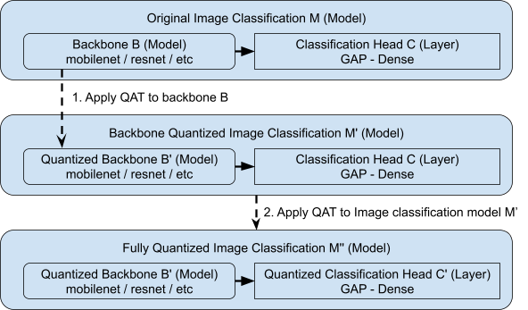
The previous QAT API assumed that the model only contained built-in layers. To support nested functional models, we apply the QAT method to different parts of the model individually. For example, to apply QAT to an image classification model (M) in the Model Garden that consists of two sub modules: the backbone network (B) and the classification head (C). Here B is a nested model within M, and C is a layer. Both B and C only contain built-in layers. Instead of directly quantizing the entire classification model M, we quantize the backbone B and classification head C individually. First, we apply QAT to backbone B only. Then we connect the quantized backbone B to its corresponding classification head C to form a new classification model, and annotate C to be quantized. Finally, we quantize the entire new model, which effectively applies QAT to the annotated classification head C.

When the backbone network also contains custom layers rather than built-in layers, we add quantized versions of those custom layers first. For example, if the backbone network (B) or the classification head (C) of the classification model (M) also contain a custom layer called MyLayer, we create its QAT counterpart called MyLayerQuantized and wrap any built-in layers within it by a quantize wrapper API. We do this recursively if there are any nested custom layers, until all built-in layers are properly wrapped.

The remaining part after applying quantize is loading the weights from the original model because the QAT-applied model contains more parameters due to additional quantization parameters. Our current solution is variable name filtering. We have added a logic to load the weights from the original model to filtered weight from the QAT-applied model to support fine-tuning from pre-trained models.

Pruning

Along with QAT, we provide two Model garden models with pruning, which is another in-training model optimization technique of MOT. Pruning sparsifies (forces a fixed portion of elements to zero) the given model’s weights during training for computation and storage efficiency.

Users can easily set pruning parameters in Model Garden configs. For better pruned model quality, starting pruning from a pre-trained dense model and careful tuning pruning schedule over training steps are well-known techniques. Both are available in Model Garden Pruning configs.

This work also provides an example of nested functional layer support in pruning. The way we used here using get_prunable_weight() is also applicable to any other Keras models with custom layers.

With the provided two Model Garden Pruning configs, users can quickly demonstrate pruning to ResNet50 and MobileNetV2 models for image classification. Understanding the practical usage of Pruning API and the pruning process by monitoring tensorboard are also another takeaways of this work.

Examples and Results

We support two tasks, image classification and semantic segmentation. Specifically, for QAT in image classification, we support the common MobileNet family, including MobileNetV2, MobileNetV3 (large), Multi-Hardware MobileNet (AVG), and ResNet (through quantization on common building blocks such as InvertedBottleneckBlockQuantized and BottleneckBlockQuantized). For QAT in semantic segmentation, we support MobileNetV2 backbone with DeepLab V3/V3+. For Pruning in image classification we support MobileNetV2 and ResNet. Please refer to the documentations of QAT and pruning for more details.

Create QAT Models using Model Garden

Using QAT with Model Garden is simple and straightforward. First, we train a floating point model following the standard process of training models using Model Garden. After training converges, we take the best checkpoint as our starting point to apply QAT, analogous to a finetuning stage. Soon, we will obtain a model that is more quantization friendly. Such model then can be converted to a TFLite model for on-device deployment.

For image classification, we evaluate the top-1 accuracy on the ImageNet validation set. As shown in Table 1, QAT model consistently outperforms PTQ model by a large margin, which achieves comparable latency. Notably, on models where PTQ fails to produce reasonable results (MobileNetV3), QAT is still capable of generating a strong quantized model with negligible accuracy drop.

Table 1. Accuracy and latency comparison of supported models for ImageNet classification. Latency is measured on a Samsung Galaxy S21 using 1-thread CPU. FP32 refers to the unquantized floating point TFLite model. PTQ INT8 refers to full integer post-training quantization. QAT INT8 refers to the quantized QAT model.

* PTQ fails to quantize MobileNet V3 properly due to hard-swish activation, thus leading to low accuracy.

We have a similar observation on semantic segmentation: PTQ introduces 1.3 mIoU drop, compared to FP32 model, while QAT model minimizes the drop to just 0.7 and maintains comparable latency. On average, we expect QAT will only introduce 0.5 top-1 accuracy drop for image classification and less than 1 mIoU drop for semantic segmentation.

Table 2. Accuracy and latency comparison of a MobileNet v2 + DeepLab v3 on Pascal VOC segmentation. Latency is measured on a Samsung Galaxy S21 using 1-thread CPU. FP32 refers to the unquantized floating point TFLite model. PTQ INT8 refers to full integer post-training quantization. QAT INT8 refers to the quantized QAT model.

Pruning Models in Model Garden

We support ResNet50 and MobileNet V2 for image classification. Pretrained dense models for each task are generated using the Model Garden training configs. The pruned model can be converted to the TFLite model. By simply setting a flag for sparsity in TFLite conversion, one can get a benefit of model size reduction through sparse data format.

For image classification, we again evaluate the top-1 accuracy on the ImageNet validation set, as well as the size of converted TFLite models. As sparsity level increases, the model size becomes more compact but accuracy degrades. The accuracy impact in high sparsity is more severe in parameter-efficient models like MobileNetV2.

Table 3. Accuracy and model size comparison of ResNet-50 and MobileNet v2 for ImageNet classification. Model size is measured by disk usage of saved TFLite models. Dense refers to the unpruned TFLite model, and 50% sparsity refers to the TFLite model with all prunable layers’ weights randomly pruned 50% of their elements.

Conclusions

We have presented an extension to TFMOT that offers QAT and pruning support for computer vision models in Model Garden. We highlight the ease of use and outstanding trade-offs about maintaining accuracy while keeping low latency or small model size.

While we believe this is a simple and user-friendly solution to enable QAT and pruning, we know this is just the beginning of streamlined works to provide even better usability.

Currently, supported tasks are limited to image classification and semantic segmentation. We will continue to add more support to other tasks, such as object detection and instance segmentation. We will also add more models, such as transformer based models, and improve the usability of TFMOT and Model Garden’s API. Thanks for your interest in this work.

Acknowledgements

We would like to thank everyone who contributed to this work, including Model Garden, Model Optimization, and our collaborators from Research. Special thanks to David Rim (emeritus), Ethan Kim (emeritus) from the Model Optimization team; Abdullah Rashwan, Xianzhi Du, Yeqing Li, Jaeyoun Kim, Jing Li from the Model Garden team; Yuqi Li from the on-device ML team.

Read More

Posted by Zhi An Ng and Marat Dukhan, Google

XNNPack is the default TensorFlow Lite CPU inference engine for floating-point models, and delivers meaningful speedups across mobile, desktop, and Web platforms. One of the optimizations employed in XNNPack is repacking the static weights of the Convolution, Depthwise Convolution, Transposed Convolution, and Fully Connected operators into an internal layout optimized for inference computations. During inference, the repacked weights are accessed in a sequential pattern that is friendly to the processors’ pipelines.

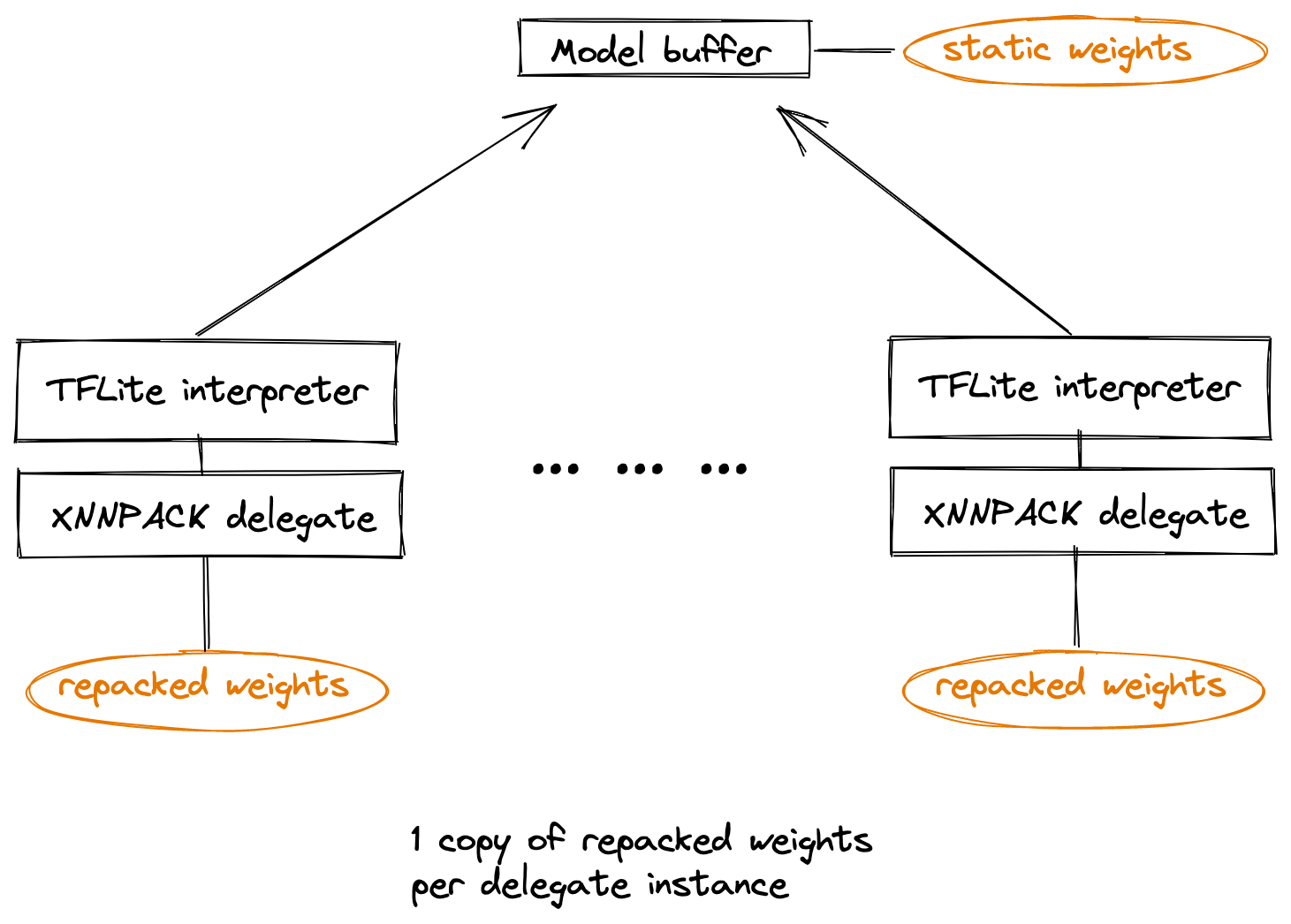
The inference latency reduction comes at a cost: repacking essentially creates an extra copy of the weights inside XNNPack. When the TensorFlow Lite model is memory-mapped, the operating system eventually releases the original copy of the weights and makes the overhead disappear. However, some use-cases require creating multiple copies of a TensorFlow Lite interpreter, each with its own XNNPack delegate, for the same model. As the XNNPack delegates belonging to different TensorFlow Lite interpreters are unaware of each other, every one of them creates its own copy of repacked weights, and the memory overhead grows linearly with the number of delegate instances. Furthermore, since the original weights in the model are static, the repacked weights in XNNPack are also the same across all instances, making these copies wasteful and unnecessary.

Weights cache is a mechanism that allows multiple instances of the XNNPack delegate accelerating the same model to optimize their memory usage for repacked weights. With a weights cache, all instances use the same underlying repacked weights, resulting in a constant memory usage, no matter how many interpreter instances are created. Moreover, elimination of duplicates due to weights cache may improve performance through increased efficiency of a processor’s cache hierarchy. Note: the weights cache is an opt-in feature available only via the C++ API.

The chart below shows the high water mark memory usage (vertical axis) of creating multiple instances (horizontal axis). It compares the baseline, which does not use weights cache, with using weights cache with soft finalization. The peak memory usage when using weights cache grows much slower with respect to the number of instances created. For this example, using weights cache allows you to double the number of instances created with the same peak memory budget.

The weights cache object is created by the TfLiteXNNPackDelegateWeightsCacheCreate function, and passed to the XNNPack delegate via the delegate options. XNNPack delegate will then use the weights cache to store repacked weights. Importantly, the weights cache must be finalized before any inference invocation.

// Example demonstrating how to create and finalize a weights cache.
std::unique_ptr<tflite::Interpreter> interpreter;
TfLiteXNNPackDelegateWeightsCache* weights_cache =
    TfLiteXNNPackDelegateWeightsCacheCreate();
TfLiteXNNPackDelegateOptions xnnpack_options =
    TfLiteXNNPackDelegateOptionsDefault();
xnnpack_options.weights_cache = weights_cache;
TfLiteDelegate* delegate =
    TfLiteXNNPackDelegateCreate(&xnnpack_options);
if (interpreter->ModifyGraphWithDelegate(delegate) != kTfLiteOk) {
    // Static weights will be packed and written into weights_cache.
}
TfLiteXNNPackDelegateWeightsCacheFinalizeHard(weights_cache);

// Calls to interpreter->Invoke and interpreter->AllocateTensors must
// be made here, between finalization and deletion of the cache.
// After the hard finalization any attempts to create a new XNNPack
// delegate instance using the same weights cache object will fail.

TfLiteXNNPackWeightsCacheDelete(weights_cache);

There are two ways to finalize a weights cache, and in the example above we use TfLiteXNNPackDelegateWeightsCacheFinalizeHard which performs hard finalization. The hard finalization has the least memory overhead, as it will trim the memory used by the weights cache to the absolute minimum. However, no new delegates can be created with this weights cache object after the hard finalization – the number of XNNPack delegate instances using this cache is fixed in advance. The other kind of finalization is a soft finalization. Soft finalization has higher memory overhead, as it leaves sufficient space in the weights cache for some internal bookkeeping. The advantage of the soft finalization is that the same weights cache can be used to create new XNNPack delegate instances, provided that the delegate instances use exactly the same model. This is useful if the number of delegate instances is not fixed or known beforehand.

// Example demonstrating soft finalization and creating multiple
// XNNPack delegate instances using the same weights cache.
std::unique_ptr<tflite::Interpreter> interpreter;
TfLiteXNNPackDelegateWeightsCache* weights_cache =
    TfLiteXNNPackDelegateWeightsCacheCreate();
TfLiteXNNPackDelegateOptions xnnpack_options =
    TfLiteXNNPackDelegateOptionsDefault();
xnnpack_options.weights_cache = weights_cache;
TfLiteDelegate* delegate =
    TfLiteXNNPackDelegateCreate(&xnnpack_options);
if (interpreter->ModifyGraphWithDelegate(delegate) != kTfLiteOk) {
    // Static weights will be packed and written into weights_cache.
}
TfLiteXNNPackDelegateWeightsCacheFinalizeSoft(weights_cache);

// Calls to interpreter->Invoke and interpreter->AllocateTensors can
// be made here, between finalization and deletion of the cache.
// Notably, new XNNPack delegate instances using the same cache can
// still be created, so long as they are used for the same model.

std::unique_ptr<tflite::Interpreter> new_interpreter;
TfLiteDelegate* new_delegate =
    TfLiteXNNPackDelegateCreate(&xnnpack_options);
if (new_interpreter->ModifyGraphWithDelegate(new_delegate) !=
    kTfLiteOk)
{
    // Repacked weights inside of the weights cache will be reused,
    // no growth in memory usage
}

// Calls to new_interpreter->Invoke and
// new_interpreter->AllocateTensors can be made here.
// More interpreters with XNNPack delegates can be created as needed.

TfLiteXNNPackWeightsCacheDelete(weights_cache);

Next steps

With the weights cache, using XNNPack for batch inference will reduce memory usage, leading to better performance. Read more about how to use weights cache with XNNPack at the README and report any issues at XNNPack’s GitHub page.

To stay up to date, you can read the TensorFlow blog, follow twitter.com/tensorflow, or subscribe to youtube.com/tensorflow. If you’ve built something you’d like to share, please submit it for our Community Spotlight at goo.gle/TFCS. For feedback, please file an issue on GitHub or post to the TensorFlow Forum. Thank you!

Read More

Posted by the TensorFlow team

As Google I/O took place, we published a lot of exciting new docs on tensorflow.org, including updates to model parallelism and model remediation, TensorFlow Lite, and the TensorFlow Model Garden. Let’s take a look at what new things you can learn about!

Counterfactual Logit Pairing

The Responsible AI team added a new model remediation technique as part of their Model Remediation library. The TensorFlow Model Remediation library provides training-time techniques to intervene on the model such as changing the model itself by introducing or altering model objectives. Originally, model remediation launched with its first technique, MinDiff, which minimizes the difference in performance between two slices of data.

New at I/O is Counterfactual Logit Pairing (CLP). This is a technique that seeks to ensure that a model’s prediction doesn’t change when a sensitive attribute referenced in an example is either removed or replaced. For example, in a toxicity classifier, examples such as “I am a man” and “I am a lesbian” should be equal and not classified as toxic.

Check out the basic tutorial, the Keras tutorial, and the API reference.

Model parallelism: DTensor

DTensor provides a global programming model that allows developers to operate on tensors globally while managing distribution across devices. DTensor distributes the program and tensors according to the sharding directives through a procedure called Single program, multiple data (SPMD) expansion.

By decoupling the overall application from sharding directives, DTensor enables running the same application on a single device, multiple devices, or even multiple clients, while preserving its global semantics. If you remember Mesh TensorFlow from TF1, DTensor can address the same issue that Mesh addressed: training models that may be larger than a single core.

With TensorFlow 2.9, we made DTensor, that had been in nightly builds, visible on tensorflow.org. Although DTensor is experimental, you’re welcome to try it out. Check out the DTensor Guide, the DTensor Keras Tutorial, and the API reference.

New in TensorFlow Lite

We made some big changes to the TensorFlow Lite site, including to the getting started docs.

Developer Journeys

First off, we now organize the developer journeys by platform (Android, iOS, and other edge devices) to make it easier to get started with your platform. Android gained a new learning roadmap and quickstart. We also earlier added a guide to the new beta for TensorFlow Lite in Google Play services. These quickstarts include examples in both Kotlin and Java, and upgrade our example code to CameraX, as recommended by our colleagues in Android developer relations!

If you want to immediately run an Android sample, one can now be imported directly from Android studio. When starting a new project, choose: New Project > Import Sample… and look for Artificial Intelligence > TensorFlow Lite in Play Services image classification example application. This is the sample that can help you find your mug…or other objects:

Model Maker

The TensorFlow Lite Model Maker library simplifies the process of training a TensorFlow Lite model using custom datasets. It uses transfer learning to reduce the amount of training data required and reduce training time, and comes pre-built with seven common tasks including image classification, object detection, and text search.

We added a new tutorial for text search. This type of model lets you take a text query and search for the most related entries in a text dataset, such as a database of web pages. On mobile, you might use this for auto reply or semantic document search.

We also published the full Python library reference.

TF Lite model page

Finding the right model for your use case can sometimes be confusing. We’ve written more guidance on how to choose the right model for your task, and what to consider to make that decision.You can also find links to models for common use cases.

Model Garden: State of the art models ready to go

The TensorFlow Model Garden provides implementations of many state-of-the-art machine learning (ML) models for vision and natural language processing (NLP), as well as workflow tools to let you quickly configure and run those models on standard datasets. The Model Garden covers both vision and text tasks, and a flexible training loop library called Orbit. Models come with pre-built configs to train to state-of-the-art, as well as many useful specialized ops.

We’re just getting started documenting all the great things you can do with the Model Garden. Your first stops should be the overview, lists of available models, and the image classification tutorial.

Other exciting things!

Don’t miss the crown-of-thorns starfish detector! Find your own COTS on real images from the Great Barrier reef. See the video, read the blog post, and try out the model in Colab yourself.

Also, there is a new tutorial on TensorFlow compression, which does lossy compression using neural networks. This example uses something like an autoencoder to compress and decompress MNIST.

And, of course, don’t miss all the great I/O talks you can watch on YouTube. Thank you!

Read More