Posts in category: Tensorflow

A guest post by Sandeep Mistry, Arm

Introduction

Emojis allow us to express emotions in the digital world, they are relatively easy to input on smartphone and tablet devices equipped with touch screen based virtual keyboards, but they are not as easy to input on traditional computing devices that have physical keyboards. To input emojis on these devices, users typically use a keyboard shortcut or mouse to bring up an on-screen emoji selector, and then use a mouse to select the desired emoji from a series of categories.

This blog will highlight an in-depth open-source guide that uses tinyML on an Arm Cortex-M based device to create a dedicated input device. This device will take real-time input from a camera and applies a machine learning (ML) image classification model to detect if the image from the camera contains a set of known hand gestures (✋, 👎, 👍, 👊). When the hand gesture is detected with high certainty, the device will then use the USB Human Interface Device (HID) protocol to “type” the emoji on the PC.

The TensorFlow Lite for Microcontrollers run-time with Arm CMSIS-NN is used as the on-device ML inferencing framework on the dedicated input device. On-device inferencing will allow us to reduce the latency of the system, as the image data will be processed at the source (instead of being transmitted to a cloud service). The user’s privacy will also be preserved, as no image data will leave the device at inference time.

Microcontrollers and Keyboards

Microcontroller Units (MCUs) are self-contained computing systems embedded in the devices you use every day, including your keyboard! Like all computing systems, they have inputs and outputs.

Block diagram of USB keyboard

Block diagram of computer vision based emoji “keyboard”

The OpenMV development platform

OpenMV is an open source (Micro) Python powered Machine Vision platform. The OpenMV product line-up consists of several Arm Cortex-M based development boards. Each board is equipped with an on-board camera and MCU. For this project, the OpenMV Cam H7 or OpenMV Cam H7 R2 board will suit our needs.

What we will need

OpenMV Cam H7 Camera (left) and microSD card (right)

• Hardware

• OpenMV Cam H7 or OpenMV Cam H7 R2 board
• MicroSD card with at least 2 MB of storage space
• USB micro cable
• Software
• OpenMV IDE
• Services
• Google Colab
• Kaggle Account

Dataset

The dataset contains ~23k image files of people performing various hand gestures over a 30 second period.

Images from the dataset will need to be relabeled as follows:

Since the swipe right and swipe left gestures in the Kaggle dataset do not correspond to any of these classes, any images in these classes will need to be discarded for our model.

Images in the Kaggle dataset are taken over a 30 second period, they might contain other gestures at the start or end of the series. For example, some of the people in the dataset started with their hands in a fist position before eventually going to the labeled gesture hand up, thumbs up and thumbs down. Other times the person in the dataset starts off with no hand gesture in frame.

We have gone ahead and manually re-labeled the images into the classes, it can be found in CSV format in the data folder on GitHub, and contains labels for ~14k images.

TensorFlow model

You can find more details on the training pipeline used here in this Colab Notebook.

Loading and Augmenting Images

Images from the dataset can be loaded as a TensorFlow Dataset using the tf.keras.utils.image_dataset_from_directory(…) API. This API supports adjusting the image’s color mode (to grayscale) and size (96×96 pixels) to meet the model’s desired input format. Built-in Keras layers for data augmentation (random: flipping, rotation, zooming, and contrast adjustments) will also be used during training.

Model Architecture

MobileNetV1 is a well-known model architecture used for image classification tasks, including the TensorLite for Microcontrollers Person detection example. This model architecture is trained on our dataset, with the same alpha (0.25) and image sizes (96x96x1) used in the Visual Wake Words Dataset paper. A MobileNetV1 model is composed of 28 layers, but a single call to the Keras tf.keras.applications.mobilenet.MobileNet(…) API can be used to easily create a MobileNetV1 model for 5 output classes and the desired alpha and input shape values:

Block Diagram of Application processing pipeline

1. Grab an image frame from the camera.
2. Get the ML model’s output for the captured image frame.
3. Filter the ML model’s output for high certainty predictions using “low activation” and “margin of confidence” techniques.
4. Use an exponential smoothing function to smooth the model’s noisy (Softmax) outputs.
5. Use the exponentially smoothed model outputs to determine if a new hand gesture is present.
6. Then “type” the associated emoji on a PC using the USB HID protocol.

Conclusion

Throughout this project we’ve covered an end-to-end flow of training a custom image classification model and how to deploy it locally to a Arm Cortex-M7 based OpenMV development board using TensorFlow Lite! TensorFlow was used in a Google Colab notebook to train the model on a re-labeled public dataset from Kaggle. After training, the model was converted into TensorFlow Lite format to run on the OpenMV board using the TensorFlow Lite for Microcontrollers run-time along with accelerated Arm CMSIS-NN kernels.

At inference time the model’s outputs were processed using model certainty techniques, and then fed output from the (Softmax) activation output into an exponential smoothing function to determine when to send keystrokes over USB HID to type emojis on a PC. The dedicated input device we created was able to capture and process grayscale 96×96 image data at just under 20 fps on an Arm Cortex-M7 processor running at 480 MHz. On-device inferencing provided a low latency response and preserved the privacy of the user by keeping all image data at the source and processing it locally.

Build one yourself by purchasing an OpenMV Cam H7 R2 board on openmv.io or a distributor. The project can be extended by fine tuning the model on your own data or applying transfer learning techniques and using the model we developed as base to train other hand gestures. Maybe you can find another public dataset for facial gestures and use it to type 😀 emojis when you smile!

A big thanks to Sparsh Gupta for sharing the Gesture Recognition dataset on Kaggle under a public domain license and my Arm colleagues Rod Crawford, Prathyusha Venkata, Elham Harirpoush, and Liliya Wu for their help in reviewing the material for this blog post and associated tutorial!

Read More

Posted by The Hugging Face Team 🤗

Language models have bloomed in the past few years thanks to the advent of the Transformer architecture. Although Transformers can be used in many NLP applications, one is particularly alluring: text generation. It caters to the practical goals of automating verbal tasks and to our dreams of future interactions with chatbots.

Text generation can significantly impact user experiences. So, optimizing the generation process for throughput and latency is crucial. On that end, XLA is a great choice for accelerating TensorFlow models. The caveat is that some tasks, like text generation, are not natively XLA-friendly.

The Hugging Face team recently added support for XLA-powered text generation in 🤗 transformers for the TensorFlow models. This post dives deeper into the design choices that had to be made in order to make the text generation models TensorFlow XLA-compatible. Through these changes to incorporate XLA compatibility, we were able to significantly improve the speed of the text generation models ~ 100x faster than before.

A Deeper Dive into Text Generation

To understand why XLA is non-trivial to implement for text generation, we need to understand text generation in more detail and identify the areas that would benefit the most from XLA.

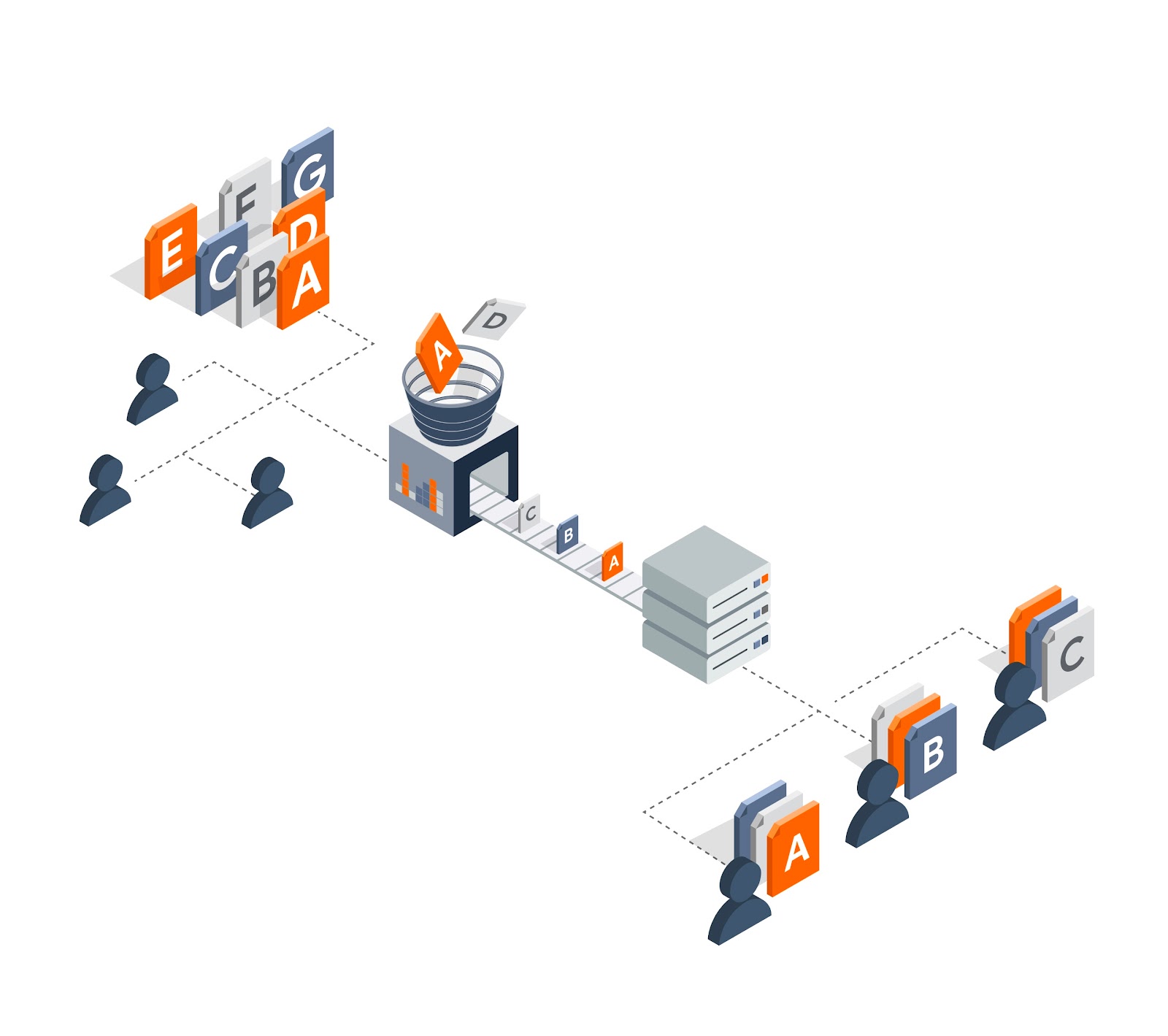
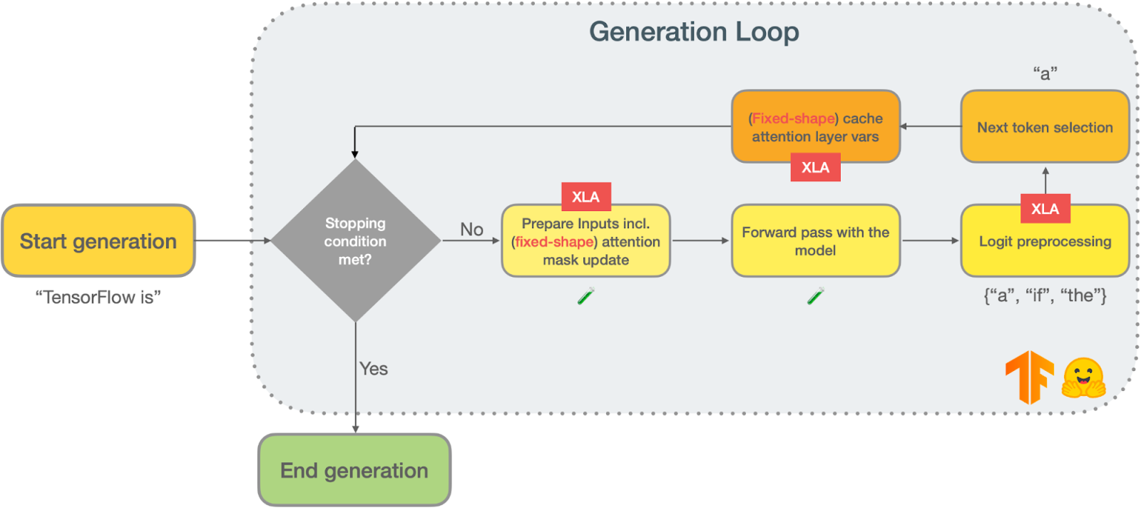
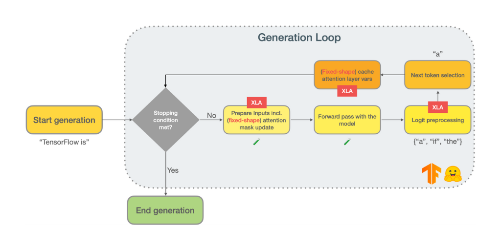
Popular models based on the Transformer architecture (such as GPT2) rely on autoregressive text generation to produce their outputs. Autoregressive text generation (also known as language modeling) is when a model is iteratively called to predict the next token, given the tokens generated so far, until some stopping criterion is reached. Below is a schematic of a typical text generation loop:

Any autoregressive text generation pipeline usually contains two main stages in addition to the model forward pass: logits processing and next token selection.

Next token selection

Next token selection is, as the name suggests, the process of selecting the token for the current iteration of text generation. There are a couple of strategies to perform next token selection:

• Greedy decoding. The simplest strategy, known as greedy decoding, simply picks the token with the highest probability as predicted by the underlying text generation model.
• Beam search. The quality of greedy decoding can be improved with beam search, where a predetermined number of best partial solutions are kept as candidates at the cost of additional resources. Beam search is particularly promising to obtain factual information from the language model, but it struggles with creative outputs.
• Sampling. For tasks that require creativity, a third strategy known as sampling is the most effective, where each subsequent input token is sampled from the probability distribution of the predicted tokens.

You can read more about these strategies in this blog post.

Logit preprocessing

Perhaps the least discussed step of text generation is what happens between the model forward pass and the next token selection. When performing a forward pass with a text generation model, you will obtain the unnormalized log probabilities for each token (also known as logits). At this stage, you can freely manipulate the logits to impart the desired behavior to text generation. Here are some examples:

• You can prevent certain tokens from being generated if you set their logits to a very large negative value;
• Token repetition can be reduced if you add a penalty to all tokens that have been previously generated;
• You can nudge sampling towards the most likely tokens if you multiply all logits by a constant smaller than one, also known as temperature scaling.

Before you move on to the XLA section of this blog post, there is one more technical aspect of autoregressive text generation that you should know about. The input to a language model is the sequence of tokens generated so far. So, if the input has N tokens, the current forward pass will repeat some attention-related computations from the previous N-1 tokens. The actual details behind these repeated computations deserve (and have) a blog post of their own, the illustrated GPT-2. In summary, you can (and should) cache the keys and the values from the masked self-attention layers where the size of the cache equals the number of input tokens obtained in the previous generation iteration.

Here we identified three keys areas that could benefit from XLA:

• Control flow
• Data structures
• Utilities accepting dynamically shaped inputs

Adjusting Text Generation for XLA

As a TensorFlow user, the first thing you must do if you want to compile your function with XLA is to ensure that it can be wrapped with a tf.function and handled with AutoGraph. There are many different paths you can follow to get it done for autoregressive text generation – this section will cover the design decisions made at Hugging Face 🤗, and is by no means prescriptive.

Switching between eager execution and XLA-enabled graph mode should come with as few surprises as possible. This design decision is paramount to the transformers library team. Eager execution provides an easy interface to the TensorFlow users for better interaction, greatly improving the user experience. To maintain a similar level of user experience, it is important for us to reduce the friction of XLA conversion.

Control flow

As mentioned earlier, text generation is an iterative process. You condition the inputs based on what has been generated, where the first generation is usually “seeded” with a start token. But, this continuity is not infinite – the generation process terminates with a stopping criterion.

For dealing with such a continuous process, we resort to while statements. AutoGraph can automatically handle most while statements with no changes, but if the while condition is a tensor, then it will be converted to a tf.while_loop in the function created by tf.function. With tf.while_loop, you can specify which variables will be used across iterations and if they are shape-invariant or not (which you can’t do with regular Python while statements, more on this later).

An advantage of using tf.while_loop for the text generation autoregressive loop is that the stopping conditions become clearly identifiable – they are the termination condition of the loop, corresponding to its cond argument. Here are two examples we resorted to tf.while_loop with explicit conditioning:

• Greedy search
• Beam search

Sometimes a for loop repeats the same operation for an array of inputs, such as in the processing of candidates for beam search. AutoGraph’s strategy will greatly depend on the type of the condition variable, but there are further alternatives that do not rely on AutoGraph. For instance, vectorization can be a powerful strategy – instead of applying a set of operations for each data point/slice, you apply the same operations across a dimension of your data. However, it has some drawbacks. Skipping operations is not desirable with vectorized operations, so it is a trade-off you should consider.

Data structures

In text generation, many data structures don’t have a static dimension that depends on how many tokens were generated up to that point. This includes:

• generated tokens themselves,
• attention masks for the tokens,
• and cached attention data as mentioned in the previous section,

among others. Although tf.while_loop allows you to use variables with varying shapes across iterations, this process will trigger re-tracing, which should be avoided whenever possible since it’s computationally expensive. You can refer to the official commentary on tracing in case you want to delve deeper.

The summary here is that if you constantly call your tf.function wrapped function with the same input tensor shape and type (even if they have different data), and do not use new non-tensor inputs, you will not incur tracing-related penalties.

At this point, you might have anticipated why loops with dynamic shapes are not desirable for text generation. In particular, the model forward pass would have to be retraced as more and more generated tokens are used as part of its input, which would be undesirable. As an alternative, our implementation of autoregressive text generation uses static shapes obtained from the maximum possible generation length. Those structures can be padded and easily ignored thanks to the attention masking mechanisms in the Transformer architecture. Similarly, tracing is also a problem when your function itself has different possible input shapes. For text generation, this problem is handled the same way: you can (and should) pad your input prompt to reduce the possible input lengths.

Transformer-based language models rely on positional embeddings for the input tokens since the Transformer architecture is permutation invariant. These positional embeddings are often derived from the size of the structures. With padded structures, that is no longer possible, as the length of the input sequences no longer matches the number of generated tokens. In fact, because different models have different ways of retrieving these positional embeddings given the position index, the most straightforward solution was to use explicit positional indexes for the tokens while generating and to perform some ad-hoc model surgery to handle them.

Here are a couple of example model surgeries that we made to make the underlying models XLA-compatible:

• T5 (pull request)
• GPT-J (pull request)

Finally, to make our users aware of the potential failure cases and limitations of XLA, we ensured adding informative in-code exceptions (an example).

To summarize, our journey from a naive TensorFlow text generation implementation to an XLA-powered one consisted of:

1. Replacing for/while Python loops conditional on tensors with tf.while_loop or vectorization;
2. Replacing if/else operations conditioned on tensors with tf.cond;
3. Creating fixed-size tensors for all tensors that had dynamic size;
4. Stopping relying on tensor shapes to obtain the positional embedding;
5. Documenting proper use of the XLA-enabled text generation.

What’s next?

The journey to XLA-accelerated TensorFlow text generation by Hugging Face 🤗 was full of learning opportunities. But more importantly, the results speak for themselves: with these changes, TensorFlow text generation can execute 100x faster than before! You can try it yourself in this Colab and can check out some benchmarks here.

Bringing XLA into your mission-critical application can greatly impact driving down costs and latency. The key to accessing these benefits lies in understanding how AutoGraph and tracing work to bring the most out of them. Have a look at the resources shared in this blog post and give it a go!

Acknowledgements

Thanks to the TensorFlow team for bringing support for XLA. Thanks to Joao Gante (Hugging Face) for spearheading the development of XLA-enabled text generation models for TensorFlow in 🤗 Transformers.

Read More

Posted by the Tensor Flow Team

TensorFlow 2.11 has been released! Highlights of this release include enhancements to DTensor, the completion of the Keras Optimizer migration, the introduction of an experimental StructuredTensor, a new warmstart embedding utility for Keras, a new group normalization Keras layer, native TF Serving support for TensorFlow Decision Forest models, and more. Let’s take a look at these new features.

TensorFlow Core

DTensor

DTensor is a TensorFlow API for distributed processing that allows models to seamlessly move from data parallelism to single program multiple data (SPMD) based model parallelism, including spatial partitioning. It gives you tools to easily train models where the model weights or inputs are so large they don’t fit on a single device. We’ve made several updates in TensorFlow v2.11.

Keras

The new Keras Optimizers API is ready

In TensorFlow 2.9, we released an experimental version of the new Keras Optimizer API, tf.keras.optimizers.experimental, to provide a more unified and expanded catalog of built-in optimizers which can be more easily customized and extended. In TensorFlow 2.11, we’re happy to share that the Optimizer migration is complete, and the new optimizers are on by default.

The old Keras Optimizers are available under tf.keras.optimizers.legacy. These will never be deleted, but they will not see any new feature additions. New optimizers will only be implemented based on tf.keras.optimizers.Optimizer, the new base class.

Most users won’t be affected by this change, but if you find your workflow failing, please check out the release notes for possible issues, and the API doc to see if any API used in your workflow has changed.

The new GroupNormalization layer

TensorFlow 2.11 adds a new group normalization layer, keras.layers.GroupNormalization. Group Normalization divides the channels into groups and computes within each group the mean and variance for normalization. Empirically, its accuracy can be more stable than batch norm in a wide range of small batch sizes, if learning rate is adjusted linearly with batch sizes. See the API doc for more details, and try it out!

A diagram showing the differences between normalization techniques.

Warmstart embedding utility

TensorFlow 2.11 includes a new utility function: keras.utils.warmstart_embedding_matrix. It lets you initialize embedding vectors for a new vocabulary from another set of embedding vectors, usually trained on a previous run.

TensorFlow Decision Forests

With the release of TensorFlow 2.11, TensorFlow Serving adds native support for TensorFlow Decision Forests models. This greatly simplifies serving TF-DF models in Google Cloud and other production systems. Check out the new TensorFlow Decision Forests and TensorFlow Serving tutorial, and the new Making predictions tutorial, to learn more.

And did you know that TF-DF comes preinstalled in Kaggle notebooks? Simply import TF-DF with import tensorflow_decision_forests as tfdf and start modeling.

TensorFlow Lite

TensorFlow Lite now supports new operations including tf.unsorted_segment_min, tf.atan2 and tf.sign. We’ve also updated tfl.mul to support complex32 inputs.

Structured Tensor

The tf.experimental.StructuredTensor class has been added. This class provides a flexible and TensorFlow-native way to encode structured data such as protocol buffers or pandas dataframes. StructuredTensor allows you to write readable code that can be used with tf.function, Keras, and tf.data. Here’s a quick example.

You can learn more in the API doc linked above.

Coming soon

Deprecating Estimator and Feature Column

Effective with the release of TensorFlow 2.12, TensorFlow 1’s Estimator and Feature Column APIs will be considered fully deprecated, in favor of their robust and complete equivalents in Keras. As modules running v1.Session-style code, Estimators and Feature Columns are difficult to write correctly and are especially prone to behave unexpectedly, especially when combined with code from TensorFlow 2.

As the primary gateways into most of the model development done in TensorFlow 1, we’ve taken care to ensure their replacements have feature parity and are actively supported. Going forward, model building with Estimator APIs should be migrated to Keras APIs, with feature preprocessing via Feature Columns specifically migrated to Keras’s preprocessing layers – either directly or through the TF 2.12 one-stop utility tf.keras.utils.FeatureSpace built on top of them.

Deprecation will be reflected throughout the TensorFlow documentation as well as via warnings raised at runtime, both detailing how to avoid the deprecated behavior and adopt its replacement.

Deprecating Python 3.7 Support after TF 2.11

TensorFlow 2.11 will be the last TF version to support Python 3.7. Since TensorFlow depends on NumPy, we are aiming to follow numpy’s Python version support policy which will benefit our internal and external users and keep our software secure. Additionally, a few vulnerabilities reported recently required that we bump our numpy version, which turned out not compatible with Python 3.7, further supporting the decision to drop support for Python 3.7.

Next steps

Check out the release notes for more information. To stay up to date, you can read the TensorFlow blog, follow twitter.com/tensorflow, or subscribe to youtube.com/tensorflow. If you’ve built something you’d like to share, please submit it for our Community Spotlight at goo.gle/TFCS. For feedback, please file an issue on GitHub or post to the TensorFlow Forum. Thank you!

Read More

Posted by The TensorFlow Team

We’re excited to announce that our Women in Machine Learning Symposium is back for the second year in a row! And you’re invited to join us virtually from 9AM – 1PM PT on December 7, 2022.

The Women in ML Symposium is an inclusive event for people to learn how to get started in machine learning and find a community of practitioners in the field. Last year, we highlighted career growth, finding community, and we also heard from leaders in the ML space.

This year, we’ll focus on coming together to learn the latest machine learning tools and techniques, get the scoop on the newest ML products from Google, and learn directly from influential women in ML. Our community strives to celebrate all intersections; as such, this event is open to everyone: practitioners, researchers, and learners alike.

Our event will have content for everyone with a keynote, special guest speakers, lightning talks, workshops and a fireside chat with Anitha Vijayakumar, Divya Jain, Joyce Shen, and Anne Simonds. We’ll feature stable diffusion with KerasCV, TensorFlow Lite for Android, Web ML, MediaPipe, and much more.

Read More

Posted by Jianhui Li, Zhoulong Jiang, Yiqiang Li from Intel, Penporn Koanantakool from Google

The ubiquity of deep learning motivates development and deployment of many new AI accelerators. However, enabling users to run existing AI applications efficiently on these hardware types is a significant challenge. To reach wide adoption, hardware vendors need to seamlessly integrate their low-level software stack with high-level AI frameworks. On the other hand, frameworks can only afford to add device-specific code for initial devices already prevalent in the market – a chicken-and-egg problem for new accelerators. Inability to upstream the integration means hardware vendors need to maintain their customized forks of the frameworks and re-integrate with the main repositories for every new version release, which is cumbersome and unsustainable.

Recognizing the need for a modular device integration interface in TensorFlow, Intel and Google co-architected PluggableDevice, a mechanism that lets hardware vendors independently release plug-in packages for new device support that can be installed alongside TensorFlow, without modifying the TensorFlow code base. PluggableDevice has been the only way to add a new device to TensorFlow since its release in TensorFlow 2.5. To bring feature-parity with native devices, Intel and Google also added a profiling C interface to TensorFlow 2.7. The TensorFlow community quickly adopted PluggableDevice and has been regularly submitting contributions to improve the mechanism together. Currently, there are 3 PluggableDevices. Today, we are excited to announce the latest PluggableDevice – Intel® Extension for TensorFlow*.

Figure 1. Intel Data Center GPU Flex Series

Intel® Extension for TensorFlow* accelerates TensorFlow-based applications on Intel platforms, focusing on Intel’s discrete graphics cards, including Intel® Data Center GPU Flex Series (Figure 1) and Intel® Arc™ graphics. It runs on Linux and Windows Subsystem for Linux (WSL2). Figure 2 illustrates how the plug-in implements PluggableDevice interfaces with oneAPI, an open, standard-based, unified programming model that delivers a common developer experience across accelerator architectures:

• Device management: We implemented TensorFlow’s StreamExecutor C API utilizing C++ with SYCL and some special support provided by the oneAPI SYCL runtime (DPC++ LLVM SYCL project). StreamExecutor C API defines stream, device, context, memory structure, and related functions, all of which have trivial mappings to corresponding implementations in the SYCL runtime.
• Op and kernel registration: TensorFlow’s kernel and op registration C API allows adding device-specific kernel implementations and custom operations. To ensure sufficient model coverage, we match TensorFlow native GPU device’s op coverage, implementing most performance critical ops by calling highly-optimized deep learning primitives from the oneAPI Deep Neural Network Library (oneDNN). Other ops are implemented with SYCL kernels or the Eigen math library. Our plug-in ports Eigen to C++ with SYCL so that it can generate programs to implement device ops.
• Graph optimization: The Flex Series GPU plug-in optimizes TensorFlow graphs in Grappler through Graph C API and offloads performance-critical graph partitions to the oneDNN library through oneDNN Graph API. It receives a protobuf-serialized graph from TensorFlow, deserializes the graph, identifies and replaces appropriate subgraphs with a custom op, and sends the graph back to TensorFlow. When TensorFlow executes the processed graph, the custom ops are mapped to oneDNN’s optimized implementation for their associated oneDNN Graph partitions.
• Profiler: The Profiler C API lets PluggableDevices communicate profiling data in TensorFlow’s native profiling format. The Flex Series GPU plug-in takes a serialized XSpace object from TensorFlow, fills the object with runtime data obtained through the oneAPI Level Zero low-level device interface, and returns the object back to TensorFlow. Users can display the execution profile of specific ops on The Flex Series GPU with TensorFlow’s profiling tools like TensorBoard.

Figure 2. How Intel® Extension for TensorFlow* implements PluggableDevice interfaces with oneAPI software components

Read More

A guest post by Matthias Hertel and Annie Tallund of Arm

Microcontrollers power the world around us. They come with low memory resources and high requirements for energy efficiency. At the same time, they are expected to perform advanced machine learning interference in real time. In the embedded space, countless engineers are working to solve this challenge. The powerful Arm Cortex-M-based microcontrollers are a dedicated platform, optimized to run energy-efficient ML. Arm and the TensorFlow Lite Micro (TFLM) team have a long-running collaboration to enable optimized inference of ML models on a variety of Arm microcontrollers.

Additionally, with well-established technologies like CMSIS-Pack, the TFLM library is ready to run on to 10000+ different Cortex-M microcontroller devices with almost no integration effort. Combining these two offers a great variety of platforms and configurations. In this article, we will describe how we have collaborated with the TFLM team to use Arm Virtual Hardware (AVH) as part of the TFLM projects open-source continuous integration (CI) framework to verify many Arm-based processors with TFLM. This enables developers to test their projects on Arm intellectual property IP without the additional complexity of maintaining hardware.

Arm Virtual Hardware – Models for all Cortex-M microcontrollers

Arm Virtual Hardware (AVH) is a new way to host Arm IP models that can be accessed remotely. In an ML context, it offers a platform to test models without requiring the actual hardware. The following Arm M-profile processors are currently available through AVH:

• Cortex-M0, Cortex-M0+
• Cortex-M3, Cortex-M4, Cortex-M7
• Cortex-M23, Cortex-M33

Arm Corstone is another virtualization technology, in the form of a silicon IP subsystem, helping developers verify and integrate their devices. The Corstone framework builds the foundation for many modern Cortex-M microcontrollers. AVH supports multiple platforms including Corstone-300, Corstone-310 and Corstone-1000. The full list of supported platforms can be found here.

Through Arm Virtual Hardware, these building blocks are available as Amazon Machine Image (AMI) on Amazon Web Services (AWS) Marketplace and locally through Keil MDK-Professional.

The Arm Virtual Hardware end-to-end workflow, from developer to the cloud.

GitHub Actions and Arm Virtual Hardware

GitHub Actions provides a popular CI solution for open-source projects, including TensorFlow Lite Micro. The AVH technology can be integrated with the GitHub Actions runner and that can be used to run tests on the different Arm platforms as natively compiled code without the need to have the hardware available.

Let’s get into how it’s done!

Defining a AVH use-case through a GitHub Actions workflow

Overview

Over the past year, we have made it possible to set up Arm IP verification in GitHub Actions. We will walk you through the steps needed to perform this integration with TFLM. The same process can be repeated for other open-source projects that use GitHub Actions as well.

A GitHub workflow file (such as Corstone-300 workflow in the TFLM repository) can be used to run code on an AWS EC2 instance, which has Arm IP installed. This workflow builds the TFLM project with Corstone-300 as a target, and runs the unit tests using both GCC and armclang, displaying the results directly in the GitHub UI via a hierarchical process as visualized below.

The workflow contains one or more jobs, which points to a file containing steps. The steps are defined in a separate file (cortex_m_corstone_300_avh.yml). In our example, the steps will then point to a test script (test_cortex_m_corstone_300.sh), which is sent using an Arm-provided API (AVH Client) to the AWS instance where it is then executed accordingly. The script will send back output, which is obtained by the AVH client and can be displayed in the GitHub Actions UI.

Depending on the nature of the use case, this can happen one or several times, which all depends on the number of jobs and steps defined. In the Corstone-300 case, we use a single job with steps that will only run one test script only. This is not a limitation however, as visualized in the flowchart above.

Connecting the GitHub Actions runner to the AWS EC2 instance running AVH

The AWS credentials are configured to allow the AVH client to connect to the AWS EC2 instance, though there are various other ways to authenticate with AWS services. These include adding the AWS keypair onto GitHub secrets, or using an allow-listed GitHub repository to ordinate a predefined role, as shown here.

Read More

Posted by the TensorFlow team

We’ve started planning the future of TensorFlow! In this article, we’d like to share our vision.

We open-sourced TensorFlow nearly seven years ago, on November 9, 2015. Since then, thanks to thousands of open-source contributors and our incredible community of Google Developer Experts, community organizers, researchers, and educators around the globe, TensorFlow has come to define its category. 

Today, TensorFlow is the most-used machine learning platform, adopted by millions of developers. It’s the 3rd most-starred software repository on GitHub (right behind Vue and React) and the most-downloaded machine learning package on PyPI. It has brought machine learning to the mobile ecosystem: TFLite now runs on four billion devices (maybe on yours, too!). TensorFlow has also brought machine learning to the Web: TensorFlow.js is now downloaded 170 thousand times weekly.

Across Google’s product lineup, TensorFlow powers virtually all production machine learning, from Search, GMail, YouTube, Maps, Play, Ads, Photos, and many more. Beyond Google, at other Alphabet companies, TensorFlow and Keras enable the machine intelligence in Waymo’s self-driving cars. 

In the broader industry, TensorFlow powers machine learning systems at thousands of companies, including most of the largest machine learning users in the world – Apple, ByteDance, Netflix, Tencent, Twitter, and countless more. And in the research world, every month, Google Scholar is indexing over 3,000 new scientific publications that mention TensorFlow or Keras.

Today, our user base and developer ecosystem are larger than ever, and growing!

We see the growth of TensorFlow not just as an achievement to celebrate, but as an opportunity to go further and deliver more value for the machine learning community.

Our goal is to provide the best machine learning platform on the planet. Software that will become a new superpower in the toolbox of every developer. Software that will turn machine learning from a niche craft into an industry as mature as web development.

To achieve this, we listen to the needs of our users, anticipate new industry trends, iterate on our APIs, and work to make it increasingly easy for you to innovate at scale. In the same way that TensorFlow originally helped the rise of deep learning, we want to continue to facilitate the evolution of machine learning by giving you the platform that lets you push the boundaries of what’s possible. Machine learning is evolving rapidly, and so is TensorFlow.

Today, we’re excited to announce we’ve started working on the next iteration of TensorFlow that will enable the next decade of machine learning development. We are building on TensorFlow’s class-leading capabilities, and focusing on four pillars.

Four pillars of TensorFlow

Fast and scalable

• XLA Compilation. We are focusing on XLA compilation and aim to make most model training and inference workflows faster on GPU and CPU, building on XLA’s performance wins on TPU. We intend for XLA to become the industry-standard deep learning compiler, and we’ve opened it up to open-source collaboration as part of the OpenXLA initiative.
• Distributed computing. We are investing in DTensor, a new API for large-scale model parallelism. DTensor unlocks the future of ultra-large model training and deployment and allows you to develop your model as if you were training on a single device, even while using multiple clients. DTensor will be unified with the tf.distribute API, allowing for flexible model and data parallelism.
• Performance optimization. Besides compilation, we are also further investing in algorithmic performance optimization techniques such as mixed-precision and reduced-precision computation, which can deliver considerable speed ups on GPUs and TPUs.

Applied ML

• New tools for CV and NLP. We are investing in our ecosystem for applied ML, in particular via the KerasCV and KerasNLP packages which offer modular and composable components for applied CV and NLP use cases, including a large array of state-of-the-art pretrained models.
• Developer resources. We are adding more code examples, guides, and documentation for popular and emerging applied ML use cases. We aim to increasingly reduce the barrier to entry of ML and turn it into a tool in the hands of every developer.

Ready to deploy

• Easier exporting. We are making it even easier to export to mobile (Android or iOS), edge (microcontrollers), server backends, or JavaScript. Exporting your model to TFLite and TF.js and optimizing its inference performance will be as easy as a call to `model.export()`.
• C++ API for applications. We are developing a public TF2 C++ API for native server-side inference as part of a C++ application.
• Deploy JAX models. We are making it easier for you to deploy models developed using JAX with TensorFlow Serving, and to mobile and the web with TensorFlow Lite and TensorFlow.js. 

Simplicity

• NumPy API. As the field of ML expanded over the last few years TensorFlow’s API surface also increased, not always in ways that are consistent or simple to understand. We are working actively on consolidating and simplifying these APIs. For example, we will be adopting the NumPy API standard for numerics. 
• Easier debugging. A framework isn’t just its API surface, it’s also its debugging experience. We aim at minimizing the time-to-solution for developing any applied ML system by focusing on better debugging capabilities.

The future of TensorFlow will be 100% backwards-compatible

We want TensorFlow to serve as a bedrock foundation for the machine learning industry to build upon. We see API stability as our most important feature. As an engineer who relies on TensorFlow as part of their product, as a builder of a TensorFlow ecosystem package, you should be able to upgrade to the latest TensorFlow version and immediately start benefiting from its new features and performance improvements – without fear that your existing codebase might break. As such, we commit to full backwards compatibility from TensorFlow 2 to the next version – your TensorFlow 2 code will run as-is. There will be no conversion script to run, no manual changes to apply.

Timeline

We plan to release a preview of the new TensorFlow capabilities in Q2 2023 and will release the production version later in the year. We will publish regular updates on our progress in the meantime. You can follow our progress via the TensorFlow blog, and on the TensorFlow YouTube channel.

Your feedback is welcome

We want to hear from you! For questions or feedback, please reach out via the TensorFlow forum.

Read More

Posted by Hannes Hapke and Robert Crowe

Startup companies building Machine Learning-based services and products require production-level infrastructure for training and serving their models. This can be especially challenging for small teams that are spread thin and need to innovate and grow quickly. TFX (TensorFlow Extended) provides a range of options to mitigate these challenges. In this blog post, you will learn how the San Francisco-based FinTech startup Digits has benefitted from applying TFX early, how TFX helps Digits grow, and how other startups can benefit from TFX too.

TFX is a set of libraries that streamline the development and deployment of production machine learning models, including implementing automated training pipelines. You might already be aware of major companies like Alphabet (including Google and Waze), Spotify, or Twitter successfully leveraging TFX to manage their machine learning pipelines. But TFX also has enormous benefits for medium-stage startups, like Digits.

Before we dive into how we are using TFX at Digits, let’s introduce a conceptual software design question that every startup will face: Choosing between tactical and strategic programming (introduced by John Ousterhout in “A Philosophy of Software Design”). In his analysis, Ousterhout shows that strategic programming is a much more sustainable approach for long-term success: even though it takes more time to get to an initial release, strategic programming will help make the complexity of a growing codebase more manageable.

Source: “A Philosophy of Software Design”, John Ousterhout, 2018

At Digits, we found that the same concept applies to machine learning. While we could train machine learning models in a minimal Jupyter notebooks-based setup, this system would become increasingly hard to manage as complexity increases. In this scenario, any initial wins of a rapidly trained machine learning model would dwindle as the company grows. Therefore, we invested heavily in our ML engineering setup from the start:

1. We developed ML-specific workflows and created a clear distinction between ML experiments and production-ready ML.
2. We invested heavily in ensuring we use tools like TFX, ML Metadata Store, and Google Cloud’s Vertex AI as efficiently as possible.
3. We automated our model deployment processes to remove human shortcuts and errors.

Ousterhout found that strategic programming requires more upfront time, but developers will benefit from lower system complexity. For example, we have spent roughly 2-3 months setting up all the ML tooling and workflows, and we recognize that it is a substantial investment.

While this might not be feasible for startups that are still trying to establish a product-market-fit, we believe that this ML strategy is the right path for startups with a growing customer base. Furthermore, it has been our experience that applying strategic programming to machine learning problems will add to the developers’ job satisfaction and increase retention among the data team in the long run (fewer rushed hotfixes, systematic model retraining, etc.).

Growing our business with TFX, we have identified three key benefits that have allowed us to optimize our ML model training and deployment in ways that have been crucial to our success as a startup:

Key benefit 1: Standardization

At Digits, we distinguish between machine learning experiments and production machine learning. The objective of an ML experiment is to develop a proof of concept model. Our engineers are free to use any framework and tooling for ML experiments as long as our security requirements are met.

When we bring a model to production and customers rely on consistent predictions, we convert these experiments to production ML models. Every time we create a production ML model, we follow a consistent project structure and use the same steps for data and model analysis as well as feature engineering. TFX is crucial in standardizing those aspects.

Because each production model follows the same standards, we can detect potential synergies between projects early. This approach enables us to share code between projects even in the earliest development stages. Standardization has increased code reusability, and new projects have a much faster ramp-up time.

Another benefit of standardizing our workflows with TFX is that we can now apply our software engineering and DevOps principles to ML projects: Pipelines that run non-periodically can be triggered by our continuous integration system. TFX pipelines then register the newly produced model with our model registry. Based on this, the continuous integration system can also update our ML-serving endpoints and automatically deploy our ML models. This way, all changes to our ML systems are tracked in our Git repository.

System components including CI

Key benefit 2: Growth

In contrast to Keras’ preprocessing layers, TFX supports feature engineering, model analysis, and data validation via Apache Beam tasks. This way we only need to implement the feature engineering once – with TFX, we can simply swap out the Apache Beam configuration when our datasets grow and we need more processing capabilities.

Startups can begin with the TFX default setup based on Apache Beam’s DirectRunner. The DirectRunner mode doesn’t allow any parallelized execution of pipeline tasks but is available without any setup time. As the startup grows, the engineering team can swap out the underlying Apache Beam Runner for a more performant system like Google Cloud’s Dataflow, Apache Spark, or Apache Flink, with minimal code changes – often only one line. While Dataflow is only available to Google Cloud customers, Apache Spark and Flink are open-source, and all major cloud providers offer managed services.

We successfully employed this strategy at Digits: We started out with Apache Beam’s DirectRunner for our initial pipelines, a setup that helped us understand how TFX can improve our ML workflows. As our company grew, the volume of data to process grew as well. To handle the increasing volume of data, TFX allowed us to switch to a different Beam runner without any friction. By building our pipelines in two phases, we didn’t have to implement TFX and the more performative and complex orchestration dependencies all at once, and saved our small initial team considerable strain.

Different Beam Runner options, depending on the data volume

Another advantage that was useful to us is how easily TFX integrates with the Google Cloud ecosystem. Google Cloud’s Vertex AI Pipeline natively supports TFX and provides all necessary pipeline infrastructure as a managed service. Instead of managing our own Kubernetes clusters, we can easily switch back and forth between pipeline runs in different Google Cloud projects. We are also not limited by cluster compute and memory limitations since we can access both GPUs and TPUs with Vertex Pipelines.

Key benefit 3: Reproducibility & Repeatability

Keeping track of all ML artifacts is key for the sustainable management of production ML models. Our goal was to track all relevant data points for all our production models. We needed to store artifacts like datasets, data splits, data validation results, feature transformations, trained models, and model analysis results. But we also didn’t want to slow down the ML team with extensive record keeping.

TFX is tightly integrated with the ML Metadata Store (MLMD) which helps us to keep track of all model details in one place. Under the hood, each TFX component in our ML pipelines records all intermediate pipeline results and metadata. We can generate model lineages for each model produced by our ML pipelines without any additional overhead. This has proven to be an indispensable tool when things move fast.

Model lineage

Digits’ Lessons Learned

While adapting TFX to our needs did take some time, we have seen this initial investment pay off over time. We are now able to convert machine learning experiments within minutes into production pipelines and continuously produce and deploy new versions of our models.

TFX helps us to make our ML codebase more modular. We have developed several custom TFX components (e.g. for model deployments, model annotations, or model tracking). Due to the modularity of the TFX components, all projects can benefit from enhancements made in a single project.

At the same time, we benefited from standardizing our production ML codebase with TFX. As a growing startup company, we found this standardization especially useful as it helped us stay on track as complexity increased. New projects now follow a highly optimized cookie-cutter approach, which has resulted in major time and labor savings. Those standardizations also allowed us to automate large parts of the model deployment processes, which in turn helped free up engineering capacities. We have found that these savings are vital for the small, flexible ML teams which are common in startups. 

Using TFX also has allowed us to future-proof our MLOps tooling. The fact that TFX uses Apache Beam under the hood gave us confidence that we don’t need to reengineer our MLOps setup as the company grows. 

TFX, its metadata store, and its Google Cloud integrations have helped us reproduce models from given artifacts and made it much easier to accurately recreate any previous ML models whenever needed.

The experience of growing Digits with TFX has convinced us that any company that is serious about machine learning can benefit from TFX – at every step along the way, from small startups to large corporations.

For more information

To learn more about TFX, check out the TFX website, join the TFX discussion group, dive into other posts in the TFX blog, watch our TFX playlist on YouTube, or subscribe to the TensorFlow channel.

Read More

Posted by Sujit Sanjeev, Product Manager, Robert Little, Sustainability Program Manager, Umair Sabir, Machine Learning Engineer

Have you ever been confused about how to file your taxes? Perplexed when assembling furniture? Unsure about how to understand your partner? It turns out that many of us find the act of recycling as more confusing than all of the above. As a result, we do a poor job of recycling right, with less than 10% of our global resources recycled, and tossing 1 of every 5 items (~17%) in a recycling bin that shouldn’t be there. That’s bad news for everyone — recycling facilities catch fire, we lose billions of dollars in recyclable material every year — and at an existential level, we miss an opportunity to leverage recycling as an impactful tool to combat climate change. With this context in mind, we asked ourselves – how might we use the power of technology to ensure that we recycle more and recycle right?

As the world population grows and urbanizes, waste production is estimated to reach 2.6 billion tons a year in 2030, an increase from its current level of around 2.1 billion tons. Efficient recycling strategies are critical to foster a sustainable future.

The facilities where our waste and recyclables are processed are called “Material Recovery Facilities” (MRFs). Each MRF processes tens of thousands of pounds of our societal “waste” every day, separating valuable recyclable materials like metals and plastics from non-recyclable materials. A key inefficiency within the current waste capture and sorting process is the inability to identify and segregate waste into high quality material streams. The accuracy of the sorting directly determines the quality of the recycled material; for high-quality, commercially viable recycling, the contamination levels need to be low. Even though the MRFs use various technologies alongside manual labor to separate materials into distinct and clean streams, the exceptionally cluttered and contaminated nature of the waste stream makes automated waste detection challenging to achieve, and the recycling rates and the profit margins stay at undesirably low levels.

Enter what we call “CircularNet”, a set of models that lowers barriers to AI/ML tech for waste identification and all the benefits this new level of transparency can offer.

Our goal with CircularNet is to develop a robust and data-efficient model for waste/recyclables detection, which can support the way we identify, sort, manage, and recycle materials across the waste management ecosystem. Models such as this could potentially help with:

Better understanding and capturing more value from recycling value chains

Increasing landfill diversion of materials

Identifying and reducing contamination in inbound and outbound material streams

Challenges

Processing tens of thousands of pounds of material every day, Material Recovery Facility waste streams present a unique and ever-changing challenge: a complex, cluttered, and diverse flow of materials at any given moment. Additionally, there is a lack of comprehensive and readily accessible waste imagery datasets to train and evaluate ML models.

The models should be able to accurately identify different types of waste in “real world” conditions of a MRF – meaning identifying items despite severe clutter and occlusions, high variability of foreground object shapes and textures, and severe object deformation.

In addition to these challenges, others that need to be addressed are visual diversity of foreground and background objects that are often severely deformed, and fine-grained differences between the object classes (e.g. brown paper vs. cardboard; or soft vs. rigid plastic).

There also needs to be consistency while tracking recyclables through the recycling value chain e.g. at point of disposal, within recycling bins and hauling trucks, and within material recovery facilities.

Solution

The CircularNet model is built to perform Instance Segmentation by training on thousands of images with the Mask R-CNN algorithm. Mask R-CNN was implemented from the TensorFlow Model Garden, which is a repository consisting of multiple models and modeling solutions for Tensorflow users.

By collaborating with experts in the recycling industry, we developed a customized and globally-applicable taxonomy of material types (e.g. “paper” “metal”,”plastic”, etc.) and material forms (e.g. “bag”, “bottle”, “can”, etc.), which is used to annotate training data for the model. Models were developed to identify material types, material forms and plastic types (HDPE, PETE, etc). Unique models were trained for different purposes, thus helping achieve better accuracy (when harmonized and flexibility to cater to different applications). The models are trained with various backbones such as ResNet, MobileNet and, SpineNet.

To train the model on distinct waste and recyclable items, we have collaborated with several MRFs and have started to accumulate real-world images. We plan to continue growing the number and geographic locations of our MRF and waste management ecosystem partnerships in order to continue training the model across diverse waste streams.

Here are a few details on how our model was trained.

• Data importing, cleaning and pre-processing
• Once the data was collected, the annotation files had to be converted into COCO JSON format. All noise, errors and incorrect labels were removed from the COCO JSON file. Corrupt images were also removed both from the COCO JSON and dataset to ensure smooth training.
• The final file is converted to the TFRecord format for faster training
• Training
• Mask RCNN was trained using the Model Garden repository on Google Cloud Platform.
• Hyper parameter optimization was done by changing image size, batch size, learning rate, training steps, epochs and data augmentation steps
• Model conversion 
• Final checkpoints achieved after training the model were converted to both saved model and TFLite model formats to support server side and edge side deployments
• Model deployment 
• We are deploying the model on Google Cloud for server side inferencing and on edge computing devices
• Visualization

Three ways in which the CircularNet model characterizes recyclables: Form, Material, & Plastic Type

• Model identifying the material type (Ex. “Plastic”)

• Model identifying the product form of the material (Ex. “Bottle”)

• Model identifying the types of plastics (Ex. “HDPE”)

How to use the CircularNet model

All the models are available with guides and their respective colab scripts for pre-processing, training, model conversion, inference and visualization are available in the Tensorflow Model Garden repository. Pre-trained models for direct use from servers, browsers or mobile devices are available on TensorFlow Hub.

Conclusion

We hope the model can be deployed by, tinkered with, and improved upon by various stakeholders across the waste management ecosystem. We are in the early days of model development. By collaborating with a diverse set of stakeholders throughout the material recovery value chain, we can better create a more globally applicable model. If you are interested in collaborating with us on this journey, please reach out to waste-innovation-external@google.com.

Acknowledgement

A huge thank you to everyone who’s hard work made this project possible! We couldn’t have done this without partnering with the recycling ecosystem.

Special thanks to Mark McDonald, Fan Yang, Vighnesh Birodkar and Jeff Rechtman

Read More

Posted by Wei Wei, Developer Advocate

In our previous blog post Building a board game app with TensorFlow: a new TensorFlow Lite reference app, we showed you how to use TensorFlow and TensorFlow Agents to train a reinforcement learning (RL) agent to play a simple board game ‘Plane Strike’. We also converted the trained model to TensorFlow Lite and then deployed it into a fully-functional Android app. In this blog, we will demonstrate a new path: train the same RL agent with Flax/JAX and deploy it into the same Android app we have built before. The complete code has been open sourced in the tensorflow/examples repository for your reference.

To refresh your memory, our RL-based agent needs to predict a strike position based on the human player’s board position so that it can finish the game before the human player does. For more detailed game rules, please refer to our previous blog.

Demo game play in ‘Plane Strike’

 

where:

• T: the number of timesteps per episode, which can vary per episode
• s_t: the state at timestep t
• a_t: chosen action at timestep t given state s
• π_θ: the policy parameterized by θ
• R(*): the reward gathered, given the policy

We define a 3-layer MLP as our policy network, which predicts the agent’s next strike position.

In our main training loop, in each iteration we use the neural network to play a round of the game, gather the trajectory information (game board positions, actions taken and rewards), discount the rewards, and then train the model with the trajectories.

Converting the Flax/JAX model to TensorFlow Lite and integrating with the Android app

After the model is trained, we use the jax2tf, a TensorFlow-JAX interoperation tool, to convert the JAX model into a TensorFlow concrete function. And the final step is to call TensorFlow Lite converter to convert the concrete function into a TFLite model.

Visualizing TFLite model converted from Flax/JAX using Netron

Read More