Posts in category: Tensorflow

Posted by Scott Main, Technical Writer, and the Coral team

In just a few years, ML models for mobile and embedded systems have come a very long way. With TensorFlow Lite (TFLite), you can now run sophisticated models that perform pose estimation and object segmentation, but these models still require a relatively powerful processor and a high-level OS in a mobile device or small computer like a Raspberry Pi. Alternatively, you can use TensorFlow Lite Micro (TFLM) on low-power microcontrollers (MCUs) to run simple models such as image and audio classification. However, the models for MCUs are much smaller, so they have limited capabilities and accuracy.

So there’s an opportunity cost when you must select between TFLM (low power but limited model performance) and regular TFLite (great model performance but higher power cost). Wouldn’t it be nice if you could get both on one board? Well, we’re happy to announce that the Coral Dev Board Micro is now available to provide exactly that.

A tiny board with big muscle

The Dev Board Micro is a microcontroller board (with a dual-core Cortex-M7 and Cortex-M4), so it’s small and power efficient, but it also includes the Coral Edge TPU™ on board, so it offers outstanding inferencing speeds for larger TFLite models. Plus, it has an on-board camera (324×324) and microphone. Naturally, there are plenty of GPIO pins and high-density connectors for add-on boards (such as our own Wireless Add-on and PoE Add-on).

The Dev Board Micro executes your models using TFLM, which supports only a subset of operations in TFLite. Even if TFLM did support all the same ops, the MCU would still be much too slow for practical applications that use complex models such as for object detection and pose estimation. However, when you compile a TFLite model for the Edge TPU, all the MCU needs to do is set the model’s input, delegate the model ops to the Edge TPU, and then read the output.

Get started

We built a new platform for the Dev Board Micro based on FreeRTOS and included compatibility with the Arduino programming language. So you can build a C++ app with CMake and flash it to the board with our command line tools, or you can write and upload an Arduino sketch with the Arduino IDE. We call this new platform coralmicro and it’s fully open sourced on GitHub.

If you choose to code with FreeRTOS, coralmicro includes all the core FreeRTOS APIs you need to build multi-tasking apps on the MCU, plus custom coralmicro APIs for interacting with GPIOs, capturing photos, listening to audio, performing multi-core processing, and much more.

Because coralmicro uses TensorFlow Lite for Microcontrollers for inferencing, running a TensorFlow Lite model on the Dev Board Micro works almost exactly the way you expect, if you’ve used TensorFlow Lite on other platforms. One difference with TFLM, compared to TFLite, is that you need to specify the ops used by your model by adding them to the MicroMutableOpResolver. For example, if your model uses 2D convolution, then you need to call AddConv2D(). This way, you conserve memory by compiling only the op kernels you actually need to run your model on the MCU. However, if your model is compiled to run on the Edge TPU, then you also need to add the Edge TPU custom op, which accounts for all the ops that run on the Edge TPU. For example, when using SSD MobileNet for object detection on the Edge TPU, only the dequantize and post-processing ops run on the MCU, and the rest are delegated to the Edge TPU custom op, so the code to set up the MicroInterpreter looks like this:

auto tpu_context = coralmicro::EdgeTpuManager::GetSingleton()->OpenDevice();
if (!tpu_context) {
  printf("ERROR: Failed to get EdgeTpu contextrn");
  vTaskSuspend(nullptr);
}

tflite::MicroErrorReporter error_reporter;
tflite::MicroMutableOpResolver<3> resolver;
resolver.AddDequantize();
resolver.AddDetectionPostprocess();
resolver.AddCustom(coralmicro::kCustomOp, coralmicro::RegisterCustomOp());

tflite::MicroInterpreter interpreter(tflite::GetModel(model.data()), resolver,
                                     tensor_arena, kTensorArenaSize,
                                     &error_reporter);

Notice that you also need to turn on the Edge TPU with OpenDevice(). Other than that and AddCustom(), the code to run an inference on the Dev Board Micro is pretty standard TensorFlow code. For more details, see our API reference for TFLM, and check out our code examples for FreeRTOS.

If you prefer to code with the Arduino IDE, we offer Arduino-style APIs for most of the same features available in FreeRTOS (multi-core processing is not available in Arduino). All you need to do is install the “Coral” boards package in the Arduino IDE’s Board Manager, select the Dev Board Micro board, and then you can browse all our examples for the Dev Board Micro in File > Examples.

You can learn more about the board and find a seller here, and start running the code examples by following our get started guide.

Read More

Posted by Shilpa Kancharla

Video data contains a rich amount of information, and has a more complex and large structure than image data. Being able to classify videos in a memory-efficient way using deep learning can help us better understand the contents within the data. On tensorflow.org, we have published a series of tutorials on how to load, preprocess, and classify video data. Here are quick links to each of these tutorials:

1. Load video data
2. Video classification with a 3D convolutional neural network
3. MoViNet for streaming action recognition
4. Transfer learning for video classification with MoViNet

Example of shape of video data, with the following dimensions: number of frames (time) x height x width x channels.

FrameGenerator to load video data

From the Load video data tutorial, let’s take the opportunity to talk about the main workhorse of the majority of these tutorials: the FrameGenerator class. Through this class, we are able to yield the tensor representation of the video and the label, or class, of the video.

Upon creating the generator class, we use the function from_generator() to feed in the data to our deep learning models. Specifically, the from_generator() API will create a dataset whose contents are generated by a generator. Using Python generators can be more memory-efficient than storing an entire sequence of data in memory. Consider creating a generator class similar to FrameGenerator and using the from_generator() API to load data into your TensorFlow and Keras models.

We use the functions parse_shape() and rearrange() from the einops library. The parse_shape() function used here maps the names of the axes to their corresponding lengths. It will return a dictionary containing this information, called old_shape. Next, we use the rearrange() function that allows you to reorder the axes for multidimensional tensors. Pass in the tensor, alongside the names of the axes you are trying to rearrange.

The notation b t h w c -> (b t) h w c here means we want to squeeze together the batch size (denoted by b) and time (denoted by t) dimensions to pass this data into the Keras Resizing layer object. When we instantiate the ResizeVideo class, we pass in the height and width values that we want to resize the frame to. Once this resizing is complete, we use the rearrange() function again to unsqueeze (using the notation (b t) h w c -> b t h w c) the batch size and time dimensions.

What’s next?

These are just a few ways you can leverage TensorFlow to work with video data in a memory-efficient manner, but such techniques aren’t just limited to video data. Medical data such as MRI scans or 3D image data also require efficient data loading and potential resizing of the shape of data. These techniques could prove useful when you are working with limited computational resources. We hope you find these tutorials helpful, and thank you for reading!

Read More

Posted by Chansung Park, Sayak Paul (ML and Cloud GDEs)

TensorFlow Extended (TFX) is a flexible framework allowing Machine Learning (ML) practitioners to iterate on production-grade ML workflows faster with reliability and resiliency. TFX’s power lies in its flexibility to run ML pipelines across different compatible orchestrators such as Kubeflow, Apache Airflow, Vertex AI Pipelines, etc., both locally and on the cloud.

In this blog post, we discuss the crucial details of building an end-to-end ML pipeline for Semantic Segmentation tasks with TFX and various Google Cloud services such as Dataflow, Vertex Pipelines, Vertex Training, and Vertex Endpoint. The pipeline also uses a custom TFX component that is integrated with Hugging Face 🤗 Hub – HFPusher. Finally, you will see how we implemented CI/CD into the mix by leveraging GitHub Actions.

Although we won’t go over all the bits of the pipeline, you can still find the code of the underlying project in this GitHub repository.

Architectural Overview

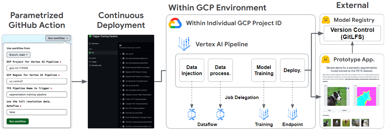
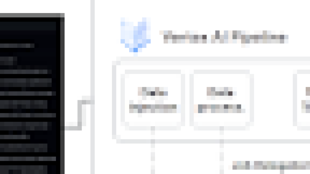
The system architecture of the project is divided into three main parts. The first part is all about the core TFX pipeline handling all the steps from data ingestion to model deployment. The second part concerns the integration between the pipeline and the external Hugging Face 🤗 Hub service. The last one is about automation and implementing CI/CD using GitHub Actions.

Figure 1. Overall system architecture (original)

It is common to open Pull Requests when proposing new features or code refactorings in separate branches. When it comes to ML projects, these changes usually affect the model and/or data. Besides running basic validation on the proposed changes (code quality, tests, etc.), we should also ensure that the changes produce a model that is better enough to replace the currently deployed model before merging (if the changes pertain to modeling). In this project, we developed a GitHub Action that is manually triggered on the merging branch with configurable parameters. This way, project stakeholders can validate performance-related changes and reliably ship the changes to production. In reality, there might be more critical measurements here, but we hope this GitHub Action proves to be a good starting point.

At the heart of any MLOps project, there is an ML pipeline. We built a simple yet complete ML pipeline with support for automatic data ingestion, data preprocessing, model training, model evaluation, and model deployment in TFX. The TFX pipeline could be run on a local environment, but we also ran it on the Vertex AI platform to replicate real-world production-grade environments.

Finally, the trained and qualified model from the ML pipeline is deployed to the Vertex AI Endpoint. The “blessed” model is also pushed to the Hugging Face Hub alongside an interactive demo via a custom HFPusher TFX component. Hugging Face Hub is a very popular place to store models and publish a fully working ML-powered interactive application for free. It is useful to showcase an application with the latest model to audit if it works as expected before going on a full production deployment.

Below, we discuss each of these components in a little more detail, discussing our design considerations and non-trivial technical aspects.

TFX Pipeline

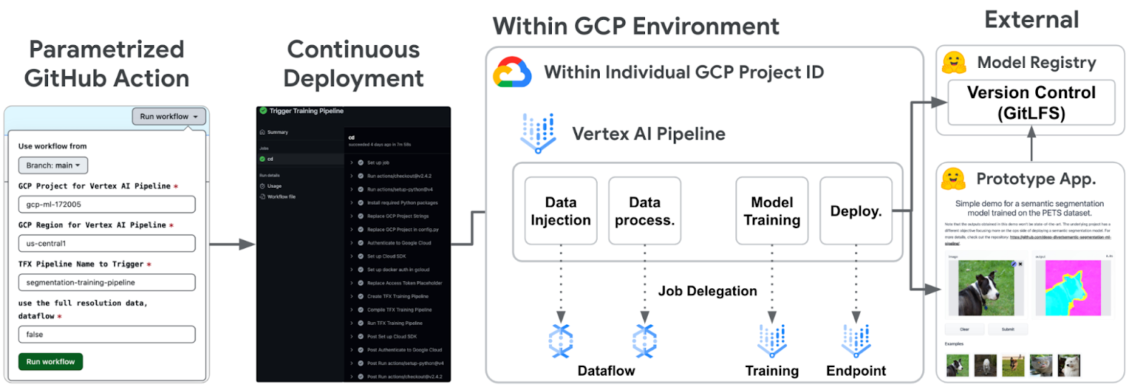
The ML pipeline is written entirely in TFX, from data ingestion to model deployment. Specifically, we used standard TFX components such as ExampleGen, ImportSchemaGen, Transform, Trainer, Evaluator, and Pusher, along with the custom HFPusher component. Let’s briefly look at the roles of each component in the context of our project.

Figure 2. Overview of the ML pipeline (original)

ExampleGen

In this project, we have prepared Pets dataset in TFRecord format with these scripts and stored them in Google Cloud Storage(GCS). ExampleGen brings the data files from GCS, splits them into training and evaluation datasets according to glob patterns, and stores them as TFRecords in GCS. Note that ExampleGen could take different data types such as CSV, TFRecord, or Parquet, then it generates datasets in a uniform format in TFRecord. It lets us handle the data uniformly inside the entire TFX pipeline. Note that since the Pets dataset is available from TF Datasets, you could also use a custom TFDS ExampleGen for this task.

ExampleGen can be integrated with Dataflow out of the box. All you need to do to benefit from Dataflow is to call with_beam_pipeline_args method with appropriate parameters such as machine type, disk size, the number of workers, and so on. For context, Dataflow is a managed service provided by Google Cloud that allows us to run Apache Beam pipelines efficiently in a fully distributed manner.

ImportSchemaGen

ImportSchemaGen imports a Protocol Buffer Text Format file that was previously automatically inferred by SchemaGen. It can also be hand-tuned to define the structure of the output data from ExampleGen.

In our case, the prepared Pets dataset has two features – image and segmentation map (label), and the size of each feature is 128×128. Therefore, we could define a schema like the one below.

Also note that in the float_domain section, we can set the value restrictions. In this project, the input data is standard RGB images, so each pixel value should be between 0 and 255. On the other hand, the pixel value of the label should be 0, 1, or 2, meaning outer, inner, and border of an object in an image, respectively.

Transform

With the help of ImportSchemaGen, the data is already shaped correctly in Transform and validated. Without ImportSchemaGen, we would have to write code to parse TFRecords and shape each feature manually inside Transform. Therefore, one line of code below is sufficient for the data preprocessing since the model in this project is built on top of MobileNetV2.

Since data preprocessing is a CPU and memory-intensive job, Transform also can be integrated with Dataflow. Just like in ExampleGen, the job could be seamlessly delegated to Dataflow by calling the with_beam_pipeline_args method.

Trainer

(Vertex) Trainer simply trains a model. We used a UNet architecture built on top of MobileNetV2 from the TensorFlow official tutorial. Since the model architecture is nothing new, let’s take a look at how it is modularized and some of the key pieces of code.

You place your modeling code in a separate file, which is supplied as a parameter to the Trainer. In this case, that file is named train.py. When the Trainer component is run, it looks for a starting point function with the name run_fn which is defined in train.py. The run_fn() function basically pulls in the training and evaluation datasets from the output of Transform, trains the UNet model ( defined in unet.py), then saves the trained model with appropriate signatures. The training process simply follows the standard Keras way – model.compile(), model.fit().

The Trainer component can be integrated with Vertex AI Training out of the box, which is a managed service to train models in a distributed system. By specifying how you would want to configure the training server clusters in the custom_config parameter of the Trainer, the training job is handled by Vertex AI Training automatically.

It is also important to notice which signatures the model exports in TensorFlow. Consider the following code snippet that saves a trained model (of the tf.keras.Model instance) into a SavedModel resource.

The signatures are functions that define how to handle given input data. For example, we have defined three different signatures. While serving_default is used during serving time, the other two are used during the model evaluation time.

• serving_default transforms a single or a batch of data points from user requests which is usually marshaled in JSON (base64 encoded) for HTTP or serialized Protocol Buffer messages for gRPC, then runs the model prediction on the data.
• transform_features applies a transformation graph obtained from the Transform component to the data produced by ExampleGen. This function will be used in the Evaluator component, so the raw evaluation inputs from ExampleGen can be appropriately transformed that the model could understand.
• from_examples performs data transformation and model prediction in a sequential manner. How data transformation is done is identical to the process of the transform_features function.

Note that the transform_features and from_examples signatures are used internally in the Evaluator component. In the next section, we explain their connections.

Evaluator

The performance of the trained model should be evaluated by certain criteria or metrics. Evaluator lets us define such metrics that not only evaluates the trained model itself but also compares the trained model to the last best model retrieved by Resolver. In other words, the trained model will be deployed only if it achieves performance above the baseline threshold and it is better than the previously deployed model. The full configurations for this project can be found here.

The reason that we had transform_features and from_examples signatures that are doing the same data preprocessing is that they are used in different situations. Evaluator runs the evaluate() method on an existing model while it runs a function (signature) specified in the signature_name on the currently trained model. Therefore, we not only need a function that transforms a given sample but also runs the evaluate() method at the same time.

Pusher

When the trained model is evaluated to be deployed, (Vertex) Pusher pushes the model to the Model Registry in Vertex AI. It also optionally creates an Endpoint and deploys the model to the endpoint out of the box. You can specify a number of different deployment-specific configurations to Pusher: machine type, GPU type, the number of GPUs, traffic splits etc.

Integration with Hugging Face 🤗 Hub

Hugging Face Hub offers ML practitioners a powerful way to store and share models, datasets, and ML applications. Since it supports seamless support for storing model artifacts with automatic version control, we developed a custom TFX component named HFPusher that:

• takes a model artifact (in the SavedModel format) and pushes that to the Hub in a separate branch for better segregation. The branch name is determined by time.time().
• creates and pushes a model card that includes attributes of the model enabling dıscovery of the models on the Hugging Face Hub platform.
• hosts an application with the model using Hugging Face Spaces given an application template referencing the branch where the model artifact was pushed to.

You can use this component anywhere after the Trainer component, but it’s recommended to use it at the end of a TFX pipeline. The HFPusher component only requires a handful of arguments consisting of two TFX artifacts and four Hugging Face specific configurations:

• Hugging Face user name
• Hugging Face access token for creating and modifying repositories on the Hugging Face Hub, which is automatically injected with GitHub Action (see the next section)
• Name of the repository to which the model artifacts will be pushed
• Model artifact as an output of a previous component such as Trainer
• Hugging Face Space specific configurations (optional)
  • Application template to host a Space application
  • Name of the repository to which the Space application will be pushed. It has the same name as the name of the model repository by default.
  • Space SDK. The default value is gradio, but it could be set to streamlit
• Model blessing artifact as an output of a previous component such as Evaluator (optional)

The Hugging Face Hub is primarily based on Git and Git-LFS. The Hugging Face team provides an easy-to-use huggingface_hub API toolkit to interact with it. That is how it provides seamless support for version control, large file storage, and interaction.

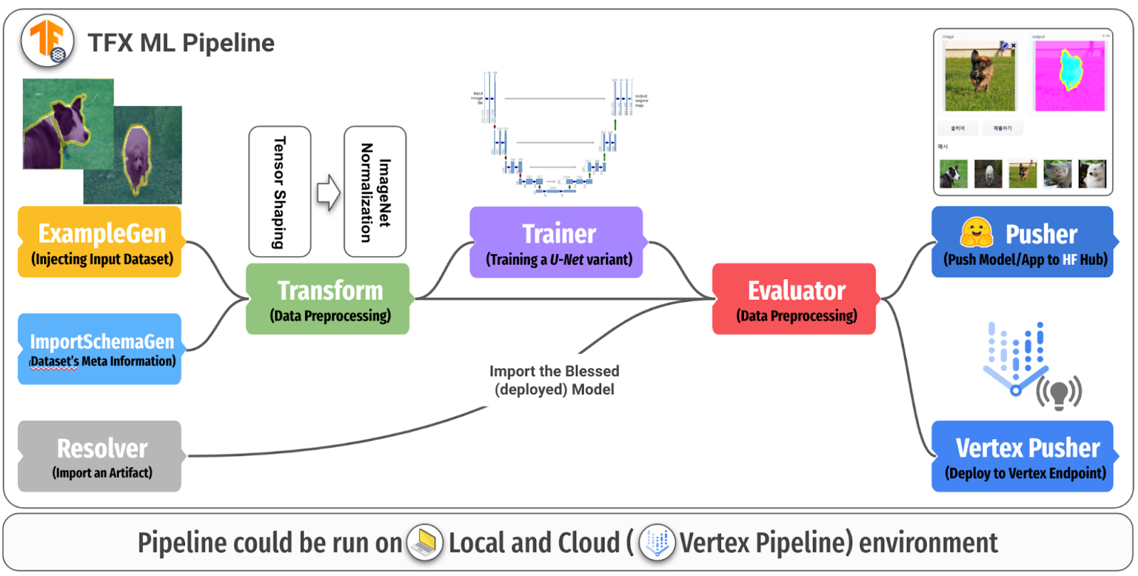
In Figures 3 and 4, we show how the model repository and the application repository (which were automatically created from a TFX pipeline) look like on the Hugging Face Hub.

Figure 3. Model versioning in Hugging Face Model Hub (original)

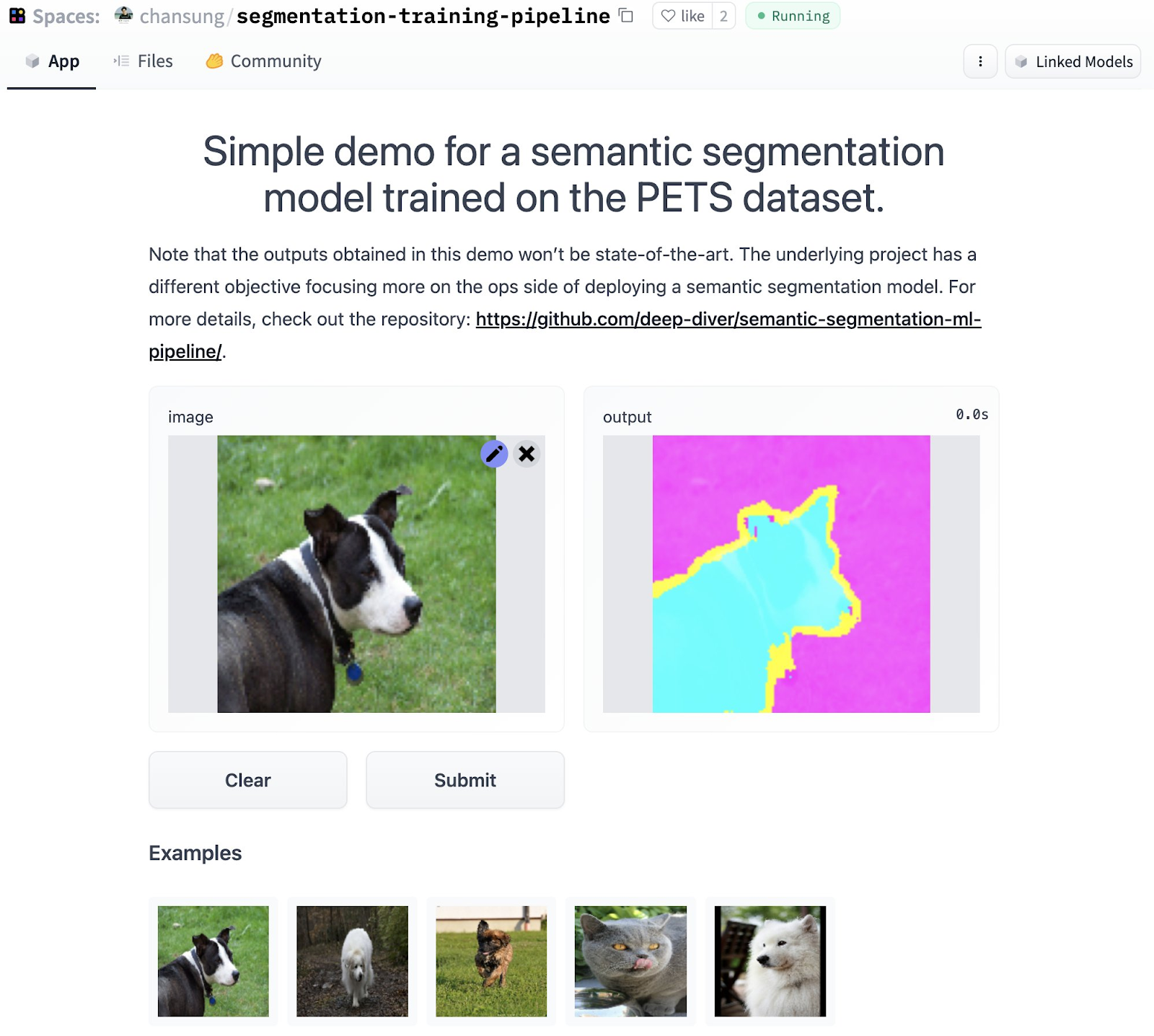
Figure 4. Automatically published application in Hugging Face Space Hub (original)

HFPusher has been contributed to the official TFX-Addons tfx-addons package. HFPusher will be available in version 0.4.0 and later in the tfx-addons package.

Automation with GitHub Actions

In the DevOps world, we usually run a number of tests on the changes introduced to ensure they’re valid enough to hit production. If the tests pass, the changes are merged and a new deployment is shipped automatically.

For an ML codebase, the changes are usually either related to data or model on a broad level. Validating these changes is quite application dependent but there could still be common grounds:

• Do the changes introduced on the modeling side lead to better performance metrics?
• Do the changes lead to faster training throughput?
• Do the data-related changes reflect some distribution better?

We focused on the first point in this project. We designed a GitHub Action workflow that can:

1. Google Cloud authentication and setup is done with google-github-actions/auth and google-github-actions/setup-gcloud GitHub Actions when a credential (JSON) is provided. In order to use appropriate credentials to the specified Google Cloud project ID, the workflow seeks for the credentials from GitHub Action Secret. Each credential is mapped to the name which is identical to the Google Cloud project ID.

2. Some of the sensitive information is replaced with envsubst command. In this project, it is required to provide a Hugging Face 🤗access token to the HFPusher component to create and update any repositories in Hugging Face 🤗 Hub. The access token is stored in GitHub Action Secret.

3. An environment variable enable_dataflow is set to “true” or “false” based on the specified parameter. By looking up the environment variable, the TFX pipeline conditionally defines dedicated parameters for Dataflow and passes them to ExampleGen and Transform components via with_beam_pipeline_args method.

4. The last part of the workflow compiles and runs the TFX pipeline on Vertex AI with the TFX CLIs as below. The tfx pipeline create CLI creates the pipeline and registers it to the local system. Furthermore, it is capable of building and pushing a Docker Image to Google Container Registry(GCR) based on a custom Dockerfile in the pipeline. Then tfx run create CLI runs the pipeline on Vertex AI with the specified Google Cloud Project ID and region.

In this case, we need to verify each PR if the suggested modification works well at the build and run times. Also, sometimes each collaborator wants to run the ML pipeline with their own Google Cloud account. Furthermore, it is better if we could conditionally delegate some heavy jobs in the ML pipeline to more dedicated Google Cloud services.

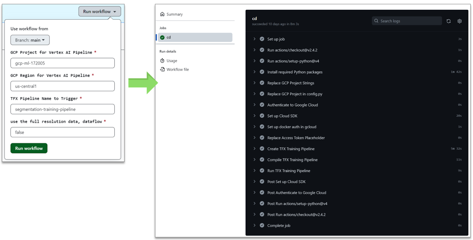
Figure 5. GitHub Action for CI/CD of ML pipeline (original)

As you may notice from Figure 5, the GitHub Action runs a workflow based on five different parameters – branch, Google Cloud project ID, cloud region, the name of TFX pipeline, and enabling the Dataflow integration.

Conclusion

In this post, we discussed how to build an end-to-end ML pipeline for semantic segmentation tasks. We leveraged TensorFlow, TFX, and Google Cloud services such as Dataflow and Vertex AI, GitHub Actions, and Hugging Face 🤗 Hub to develop a production-grade ML pipeline with external services along with semi-automatic CI/CD pipelines. We hope that you found this setup useful and reliable and that you will use this in your own ML pipeline projects.

As a future work, we will demonstrate a common MLOps scenario by extending this project. First, we’ll add more complexities to the data to simulate model performance degradation. Second, we’ll evaluate the currently deployed model to see if the model performance degradation actually happened. Last, we’ll verify the model performance is recovered after replacing the current model architecture with better ones such as DeepLabV3+ or SegFormer.

Acknowledgements

We are grateful to the ML Developer Programs team that provided Google Cloud credits to support our experiments. We thank Robert Crowe for providing us with helpful feedback and guidance. We also thank Merve Noyan who worked on integrating the model card utilities into the HFPusher component.

Read More

Posted by Ashraf Bhuiyan, AG Ramesh from Intel, Penporn Koanantakool from Google

TensorFlow 2.9.1 was the first release to include, by default, optimizations driven by the Intel® oneAPI Deep Neural Network (oneDNN) library, for 3rd Gen Intel ® 3^rd Xeon® processors (Cascade Lake). Since then, Intel and Google have continued our collaboration to introduce new TensorFlow optimizations for the next generation of Intel Xeon processors.

These optimizations accelerate TensorFlow models using the new matrix-based instructions set, Intel® Advanced Matrix Extension (AMX). The Intel AMX instructions are designed to accelerate deep learning operations such as matrix multiplication and convolutions that use Google’s bfloat16 and 8-bit low precision data types. Low precision data types are widely used and provide significant improvement over the default 32-bit floating format without significant loss in accuracy.

We are happy to announce that these features are now available as a preview in the nightly build of TensorFlow on Github, and also in the Intel optimized build. TensorFlow developers can now use Intel AMX on the 4^th Gen Intel® Xeon® Scalable processor (formerly known as Sapphire Rapids) using the existing mixed precision support available in TensorFlow. We are excited by the results – several popular AI models run up to 19x faster by moving from 3^rd Gen to 4^th Gen Intel Xeon processors using Intel AMX.

Intel’s Advanced Matrix Extension (AMX) Accelerations in 4^th Gen Intel Xeon Processor

The Intel® Advanced Matrix Extension (AMX) is an X86-based extension which introduces a new programming framework for dot products of two matrices. Intel AMX serves as an AI acceleration engine and builds on capabilities such as AVX-512 (for optimized vector operations) and Deep Learning Boost (through Vector Neural network Instructions for optimized resource utilization/caching and for lower precision AI optimizations) in previous generations of Intel Xeon processors.

In Intel AMX, a new type of 2-dimensional register file, called “tiles”, and a set of 12 new X86 instructions to operate on the tiles, are introduced. New instruction TDPBF16PS performs a dot product of bfloat16 tiles, and TDPBSSD performs dot product of signed 8-bit integer tiles. Other instructions include tile configuration and data movement to the Intel AMX unit. Further details can be found in the document published by Intel.

How to take advantage of AMX optimizations on 4^th Gen Intel Xeon.

Intel AMX optimizations are included in the official TensorFlow nightly releases. The latest stable release 2.11 includes preliminary support, however full support will be available in a subsequent stable release.

Users running TensorFlow on Intel 4^th gen Intel Xeon can take advantage of the optimizations with minimal changes:

a)    For bfloat16 mixed precision, developers can accelerate their models using Keras mixed precision API, as explained here. You can easily invoke auto mixed precision by including these lines in your code, that’s it! 

   

from tensorflow.keras import mixed_precisionpolicy = mixed_precision.Policy('mixed_bfloat16') mixed_precision.set_global_policy(policy)

b)    Using Intel AMX with 8-bit quantized models requires the models to be quantized to use int8. Any existing standard models, for example RN50, BERT, SSD-RN34 that have been previously quantized with Intel Neural Compressor will run with no changes needed.

Performance improvements

The following charts show performance improvement on a 2-socket, 56-core 4^th Gen Intel Xeon using Intel AMX low precision on various popular vision and language models, where the baseline is a 2-socket, 40-core 3^rd Gen Intel Xeon with FP32 precision. We use Intel Optimization for TensorFlow* preview and the launch_benchmark script from Model Zoo for Intel® Architecture .

Here in the chart, inference with mixed precision models on a 4^th Gen Intel Xeon was 1.9x to 9.6x faster than FP32 models on a 3^rd Gen Intel Xeon. (BS=x indicates a large batch size, depending on the model)

Training models with auto-mixed-precision on a 4th Gen Intel Xeon was 2.3x to 5.5x faster than FP32 models on a 3rd Gen Intel Xeon.

Similarly, quantized model inference on a 4^th Gen Intel Xeon was 3.3x to 19x faster than FP32 precision on a 3^rd Gen Intel Xeon.

In addition to the above popular models, we have tested 100s of other models to ensure that the performance gain is observed across the board.

Next Steps

We are working to continuously tune and improve the Intel AMX optimizations in future releases of TensorFlow. We encourage users to optimize their AI models with Intel AMX on Intel 4^th Gen processors to get a significant performance boost; not just for inference, but also for pre-training, fine tuning and transfer learning. We would like to hear from you, please provide feedback through the TensorFlow Github page or the oneAPI Deep Neural Network library GitHub page.

Acknowledgements

The results presented in this blog is the work of many people including the TensorFlow and oneDNN teams at Intel and our collaborators in Google’s TensorFlow team.

From Intel: Md Faijul Amin, Mahmoud Abuzaina, Gauri Deshpande, Ashiq Imran, Kanvi Khanna, Geetanjali Krishna, Sachin Muradi, Srinivasan Narayanamoorthy, Bhavani Subramanian, Yimei Sun, Om Thakkar, Jojimon Varghese, Tatyana Primak, Shamima Najnin, Mona Minakshi, Haihao Shen, Shufan Wu, Feng Tian, Chandan Damannagari.

From Google: Eugene Zhulenev, Antonio Sanchez, Emilio Cota.

*For configuration details see www.intel.com/performanceindex

Notices and Disclaimers:

Intel’s compilers may or may not optimize to the same degree for non-Intel microprocessors for optimizations that are not unique to Intel microprocessors. These optimizations include SSE2, SSE3, and SSSE3 instruction sets and other optimizations. Intel does not guarantee the availability, functionality, or effectiveness of any optimization on microprocessors not manufactured list by Intel. Microprocessor-dependent optimizations in this product are intended for use with Intel microprocessors. Certain optimizations not specific to Intel microarchitecture are reserved for Intel microprocessors. Please refer to the applicable product User and Reference Guides for more information regarding the specific instruction sets covered by this notice.

Read More

Posted by Jaehong Kim, Fan Yang, Shixin Luo, and Jiyang Kang

The TensorFlow Model Garden provides implementations of many state-of-the-art machine learning models for vision and natural language processing, and workflow tools to let you quickly configure and run those models on standard datasets. These models are implemented using modern best practices.

Previously, we have announced the quantization aware training (QAT) support for various on-device vision models using TensorFlow Model Optimization Toolkit (TFMOT). In this post, we introduce new SOTA models optimized using QAT in object detection, semantic segmentation, and natural language processing.

RetinaNet+MobileNetV2

A new QAT supported object detection model has been added to the Model Garden. Specifically, we use a MobileNetV2 with 1x depth multiplier as the backbone and a lightweight RetinaNet as the decoder. MobileNetV2 is a widely used mobile model backbone and we have provided QAT support since our last release. RetinaNet is the SOTA one-stage detection framework used for detection tasks and we make it more efficient on mobile devices by using separable convolution and reducing the number of filters. We train the model from scratch without any pre-trained checkpoints. 

Results show that with QAT, we can successfully preserve the model quality while reducing the latency significantly. In comparison, post-training quantization (PTQ) does not work out-of-the-box smoothly due to the complexity of the RetinaNet decoder, thus leading to low box average precision (AP).

MOSAIC

MOSAIC is a neural network architecture for efficient and accurate semantic image segmentation on mobile devices. With a simple asymmetric encoder-decoder structure which consists of an efficient multi-scale context encoder and a light-weight hybrid decoder to recover spatial details from aggregated information, MOSAIC achieves better balanced performance while considering accuracy and computational cost. MLCommons MLPerf adopted MOSAIC as the new industry standard model for mobile image segmentation benchmark.

We have added QAT support for MOSAIC as part of the open source release. In Table 2, we provide the benchmark comparison between DeepLabv3+ and MOSAIC. We can clearly observe that MOSAIC achieves better performance (mIoU: mean intersection-over-union) with significantly lower latency. The negligible gap between QAT INT8 and FP32 also demonstrates the effectiveness of QAT. Please refer to the paper for more benchmark results.

MobileBERT

MobileBERT is a thin version of BERT_LARGE, while equipped with bottleneck structures and a carefully designed balance between self-attentions and feed-forward networks. (code)

We applied QAT to the MobileBERT model to show our QAT toolkit can apply to the Transformer based mode, which has become very popular these days.

MobileBERT-EdgeTPU-XS model

Next steps

In this post, we expanded the coverage of QAT support and introduced new state-of-the-art quantized models in Model Garden for object detection, semantic segmentation, and natural language processing. TensorFlow practitioners can easily utilize these SOTA quantized models for their problems achieving lower latency or smaller model size with minimal accuracy loss.

To learn more about the Model Garden and its Model Optimization Toolkit support, check out the following blog posts:

• Introducing the Model Garden for TensorFlow 2
• Adding Quantization-aware Training and Pruning to the TensorFlow Model Garden

Model Garden provides implementation of various vision and language models, and the pipeline to train models from scratch or from checkpoints. To get started with Model Garden, you can check out the examples in the Model Garden Official repository. Model libraries in this repository are optimized for fast performance and actively maintained by Google engineers. Simple colab examples for training and inference using these models are also provided.

Acknowledgements

We would like to thank everyone who contributed to this work including the Model Garden team, Model Optimization team and Google Research team. Special thanks to Abdullah Rashwan, Yeqing Li, Hongkun Yu from the Model Garden team; Jaesung Chung from the Model Optimization team, Weijun Wang from the Google Research team.

Read More

Posted by Joana Carrasqueira, Developer Relations Program Manager

Thank you to everyone who joined us at the second Women in Machine Learning Symposium!

Last year we founded the Women in Machine Learning program, with the goal of building an inclusive space for all intersections of diversity and to give a voice and platform to women passionate about ML. Hundreds joined to share tips and insights for careers in ML, learned how to get involved in the community, contributed to open source, and much more.

This year, thousands of ML practitioners joined from all over the world. Everyone came together to learn the latest Machine Learning tools and techniques, get the scoop on the newest ML products from Google, and learn directly from several amazing women in the field.

During the keynote we announced:

• Simple ML for Sheets – Simple ML is an add-on, in beta, for Google Sheets from the TensorFlow team that helps make machine learning accessible to all. Anyone, even people without programming or ML expertise, can experiment and apply some of the power of machine learning to their data in Google Sheets with just a few clicks. Watch the demo here.
• MediaPipe Previews – We invited developers to preview low-code APIs that provide solutions to common on-device ML challenges across vision, natural language and audio. We also opened MediaPipe Studio, a web-based interface that provides a new way to prototype and benchmark ML solutions.
• TensorFlow Recommendation Systems Hub – We published a new dedicated page on TensorFlow.org where developers can find tools and guidance for building world-class recommendation systems with the TensorFlow ecosystem.
• Upcoming Sign Language AI Kaggle Competition – Our first Sign Language AI Competition to help the partners of deaf children learn to sign launches soon. Sign up to get notified when it launches.

Following is a quick recap, and workshops from the event. Thanks again.

Workshops:

This session gives participants a hands-on overview on how to get started in ML, covering various topics from introduction to ML models, to creating your first ML project. Learn how to use Codelabs and leverage technical documentation to help you getting started.

Watch Now

TensorFlow Lite in Android with Google Play Services

TensorFlow Lite is available in Google Play services runtime for all Android devices running Play services. Learn how to run ML models without statically bundling TensorFlow Lite libraries into your app and enable you to reduce the size of your apps and gain improved performance from the latest stable version of the libraries.

Watch Now

Advanced On-Device ML Made Easy with MediaPipe

Learn how MediaPipe can help you easily create custom cross-platform on-device ML solutions with low-code and no-code tools. In this session, you’ll see how to quickly try out on-device ML solutions on a web browser, then customize them in just a few lines of Python code, and easily deploy them across multiple platforms: web, Android and Python.

Watch Now

Generative Adversarial Networks (GANs) and Stable Diffusion

Watch Now

What’s Next? 

Subscribe to the TensorFlow channel on YouTube and check out the Women in Machine Learning Symposium 2022 playlist at your convenience!

Read More

Posted by Mathieu Guillame-Bert, Richard Stotz, Luiz GUStavo Martins, Ashley Oldacre, Jocelyn Becker, Glenn Cameron, and Jan Pfeifer

Today at the Women in ML Symposium thousands of ML developers and enthusiasts gathered to learn about the latest ML products from Google. Advances in machine learning (ML) technology continue to power breakthroughs in many fields. From helping to protect the Great Barrier Reef to helping amputees reclaim mobility. However, such work often requires deep ML expertise, programming experience, and time.

To make ML accessible beyond ML experts, we’ve been working on Simple ML for Sheets. Simple ML is an add-on, in beta, for Google Sheets from the TensorFlow team that helps make machine learning accessible to all. Anyone, even people without programming or ML expertise, can experiment and apply some of the power of machine learning to their data in Google Sheets with just a few clicks. From small business owners, scientists, and students to business analysts at large corporations, anyone familiar with Google Sheets can make valuable predictions automatically.

For example, if you’re a car repair shop owner who keeps records of past repairs with data points like car make, repair type, and mileage, you can use Simple ML to predict the number of hours necessary to fix a car. Scientists can also benefit from ML in countless domains. For example, if you are studying molecular aging, you can predict a person’s age based on DNA methylation data. In either use case, these ML-powered predictions are at your fingertips in just a few clicks, all via the familiar Sheets interface you use every day.

Simple ML works in three overall steps:

1. Open your data in Google Sheets.
2. Select and run the task that best describes what you want to do, like predicting missing values or spotting abnormal ones. Tasks are organized so you can use them even if you don’t know anything about Machine Learning.
3. After a few seconds, once the model has made a prediction, you can explore using the result to improve your business decisions, automate tasks, or do any of the seemingly endless applications that ML enables. If you are new to ML, remember these are just statistical predictions, of course, and may be inaccurate.

Predicting missing penguin species with Simple ML for Sheets

Even if you already know how to train and use machine learning models, Simple ML in Sheets can help make your life even easier. For instance, training, evaluating, interpreting, and exporting a model to Notebook takes only 5 clicks and as little as 10 seconds. Since Simple ML in Sheets is based on state-of-the-art ML technology that also powers TensorFlow Decision Forests , and pre-optimized, you might even get better models.

Of course, succeeding with ML involves far more than training a model and making a prediction. If you are new to ML, you should begin with Google’s free machine learning courses, including problem framing.

Because Simple ML runs on your browser your data stays right where you’re working – secure in your spreadsheet in Google Sheets. The models get automatically saved to Google Drive so you can easily share them with the rest of your team. And because Simple ML uses TensorFlow Decision Forests underneath, you can export models trained in SimpleML to the TensorFlow ecosystem!

Want to try it? Follow the introduction tutorial to get started. Then, try the add-on on your own data! Feedback is welcomed. And as always, use AI responsibly.

Read More

Posted by the TensorFlow Team

Join us tomorrow, Dec. 7, 2022, for Dr. Vivienne Ming’s session at the Women in Machine Learning Symposium at 10:25 AM PST. Register here.

Dr. Vivienne Ming explores maximizing human capacity as a theoretical neuroscientist, delusional inventor, and demented author. Over her career she’s founded 6 startups, been chief scientist at 2 others, and launched the “mad science incubator”, Socos Labs, where she explores seemingly intractable problems—from a lone child’s disability to global economic inclusion—for free.

A note from Dr. Vivienne Ming:

I have the coolest job in the whole world. People bring me problems:

• My daughter struggles with bipolar disorder, what can we do?
• What is the biggest untracked driver of productivity in our company?
• Our country’s standardized test scores go up every year; why are our citizens still underemployed?

If I think my team and I can make a meaningful difference, I pay for everything, and if we come up with a solution, we give it away. It’s possibly the worst business idea ever, but I get to nerd out with machine learning, economic modeling, neurotechnologies, and any other science or technology just to help someone. For lack of a more grown up title I call this job professional mad scientist and I hope to do it for the rest of my life.

The path to this absurd career wound through academia, entrepreneurship, parenthood, and philanthropy. In fact, my very first machine learning project as an undergrad in 1999 (yes, we were partying like it was) concerned building a lie detection system for the CIA using face tracking and expression recognition. This was, to say the least, rather morally gray, but years later I used what I’d first learned on that project to build a “game” to reunite orphaned refugees with their extended family. Later still, I helped develop an expression recognition system on Google Glass for autisttic children learning to read facial expressions.

As a grad student I told prospective advisors that I wanted to build cyborgs. Most (quite justifiably) thought I was crazy, but not all. At CMU I developed a convolutional generative model of hearing and used it to develop ML-driven improvements in cochlear implant design. Now I’m helping launch 3 separate startups mashing up ML and neurotech to augment creativity, treat Alzhiemers, and prevent postpartum depression of other neglected hormonal health challenges.

I’ve built ML systems to treat my son’s type 1 diabetes, predict manic episodes, and model causal effects in public policy questions (like, which policies improve job and patent creation by women entrepreneurs?). I’ve dragged you through all of the above absurd bragging not because I’m special but to explain why I do what I do. It is because none of this should have happened—no inventions invented, companies launched, or lives saved…mine least of all.

Just a few years before that CIA face analysis project I was homeless. Despite having every advantage, despite all of the expectations of my family and school, I had simply given up on life. The years in between taught me the most important lesson I could ever learn, which had nothing to do with inverse Wishart Distributions or Variational Autoencoder. What I learned is that life is not about me. It’s not about my happiness and supposed brilliance. Life is about our opportunities to build something bigger than ourselves. I just happen to get to build using the most overhyped and yet underappreciated technology of our time.

There’s a paradox that comes from realizing that life isn’t about you: you finally get to be yourself. For me that meant becoming a better person, a person that just happened to be a woman. (Estrogen is the greatest drug ever invented—I highly recommend it!) It meant being willing to launch products not because I thought they’d pay my rent but because I believed they should happen no matter the cost. And every year my life got better…and the AI and cooler 🙂

Machine learning is an astonishingly powerful tool, and I’m so lucky to have found it just at the dawn of my career. It is a tool that goes beyond my scifi dreams or nerd aesthetics. It’s a tool I use to help others do what I did for myself: build a better person. I’ve run ML models over trillions of data points from hundreds of millions of people and it all points at a simple truth: if you want an amazing life, you have to give it to someone else.

So, build something amazing with your ML skills. Build something no one else in the world would build because no one else can see the world the same as you. And know that every life you touch with your AI superpower will go on to touch innumerable other lives.

Read More

Posted by Wei Wei, Developer Advocate

Recommendation systems, often called recommenders as well, are a type of machine learning systems that can give users highly relevant suggestions based on the user’s interests. From recommending movies or restaurants, to highlighting news articles or entertaining videos, they help you surface compelling content from a large pool of candidates to your users, which boosts the likelihood your users interact with your products or services, broadens the content your users may consume, and increases the time your users spend within your app. To help developers better leverage our offerings in the TensorFlow ecosystem, today we are very excited to launch a new dedicated page that gathers all the tooling and learning resources for creating recommendation systems, and provides a guided path for you to choose the right products to build with.

While it is relatively straightforward to follow the Wide & Deep Learning paper and build a simple recommender using the TensorFlow WideDeepModel API, modern large scale recommenders in production usually have strict latency requirements, and thus, are more sophisticated and require a lot more than just a single API or model. The generated recommendations from these recommenders are typically a result of a complex dance of many individual ML models and components seamlessly working together. Over the years Google has open sourced a suite of TensorFlow-based tools and frameworks, such as TensorFlow Recommenders, which powers all major YouTube and Google Play recommendation surfaces, to help developers create powerful in-house recommendation systems to better serve their users. These tools are based upon Google’s cutting-edge research, extensive engineering experience, and best practices in building large scale recommenders that power a number of Google apps with billions of users.

You can start with the elegant TensorFlow Recommenders library, deploy with TensorFlow Serving, and enhance with TensorFlow Ranking and Google ScaNN. If you encounter specific challenges such as large embedding tables or user privacy protection, you will be able to find suitable solutions to overcome them from the new recommendation system page. And if you want to experiment with more advanced models such as graph neural networks or reinforcement learning, we have listed additional libraries for you as well.

This unified page is now the entry point to building recommendation systems with TensorFlow and we will keep updating it as more tools and resources become available. We’d love to hear your feedback on this initiative, please don’t hesitate to reach out via the TensorFlow forum.

Read More

A guest post by Roberta Duarte, IAG/USP

Astronomy is the science of trying to answer the Universe’s biggest mysteries. How did the Universe begin? How will it end? What is a black hole? What are galaxies and how did they form? Is life a common piece in the Universe’s puzzle? There are so many questions without answers. Machine learning can be a vital tool to answer those questions and help us unfold the Universe.

Astronomy is one of the oldest sciences. The reason is simple: we just have to look at the sky and start questioning what we are seeing. It is what astronomers have been doing for centuries. Galileo discovered a series of celestial objects after he observed the sky through the lenses of his new invention: the telescope. A few years later, Isaac Newton used Galileo’s contributions to find the Law of Universal Gravitation. With Newton’s results, we could not only understand better how the Sun affects Earth and other planets but also why we are trapped on Earth’s surface. Centuries later, Edwin Hubble found that galaxies are moving away from us and that further galaxies are moving faster than closer ones. Hubble’s findings showed that the Universe is expanding and is accelerated. These are a few examples of how studying the sky can give us some answers about the universe.

What all of them have in common is that they record data obtained from observations. The data can be a star’s luminosity, planets’ positions, or even galaxies’ distances. With technology improving the observations, more data is available to help us understand the Universe around us. Recently, the most advanced telescope, James Webb Space Telescope (JWST), was launched to study the early Universe in infrared. JWST is expected to transmit 57.2 gigabytes per day of data containing information about early galaxies, exoplanets, and the Universe’s structure.

While this is excellent news for astronomers, it also comes with a high cost. A high computational cost. In 2020, Nature published an article about big data and how Astronomy is now in an era of big data. JWST is one of the examples of how those powerful telescopes are producing huge amounts of data every day. Vera Rubin Observatory is expected to collect 20 terabytes per night. Large Arrays collect petabytes of data every year, and next-generation Large Arrays will collect hundreds of petabytes per year. In 2019, several Astro White Papers were published with the goals and obstacles in the Astronomy field predicted for the 2020s. They outlined how Astronomy needs to change in order to be prepared for the huge volume of data expected during the 2020s. New methods are required since the traditional cannot deal with the expressive number. We see problems showing up when talking about storage, software, and processing.

The storage problem may have a solution in cloud computing, eg. GCP, as noted by Nature. However, processing does not have a simple solution. The methods used to process and analyze the data need to change. It is important to note that Astronomy is a science based on finding patterns. Stars with the same redshift – an estimation of the distance of stars in space relative to us by measuring the shift of the star’s light waves towards higher frequencies – and similar composition can be considered candidates for the same population. Galaxies with the same morphology and activity or spectrum originating in the nucleus usually show the presence of black holes with similar behavior. We can even calculate the Universe’s expansion rate by studying the pattern in the spectra of different Type I Supernovae. And, what is the best tool we have to learn patterns in a lot of data? Machine Learning.

Machine learning is a tool that Astronomy can use to deal with the computational problems cited above. A data-driven approach offered by machine learning techniques may help to get analysis and results faster than traditional methods such as numerical simulations or MCMC – a statistical method of sampling from a probability distribution. In the past few years, we are seeing an interesting increase in the interaction between Astronomy and machine learning. To quantify, the keyword machine learning presented in Astronomy’s papers increased four times from 2015 to 2020 while deep learning increased 3 times each year. More specifically, machine learning was widely used to classify celestial objects and to predict spectra from given properties. Today, we see a large range of applications since discovering exoplanets, simulations of the Universe’s cosmic web, and searching for gravitational waves.

If you start adding complexity, such as electromagnetism equations to understand the magnetic fields around a black hole and general relativity equations to realistically explain the space-time there, the time can increase significantly. We are slowly reaching a barrier in black hole physics due to computational limitations where it is becoming harder and harder to realistically simulate a black hole.

Black hole research

That is where my advisor, Rodrigo Nemmen, and I started to think about a new method to accelerate black hole physics. In other words, a new method that could accelerate the numerical simulations we needed to study these extreme objects. From the beginning machine learning seems like the method with the best perspective for us. We had the data to feed into a machine learning algorithm and there were successful cases in the literature simulating fluids using machine learning. But never around a black hole. It was worth giving it a shot. We began a collaboration with João Navarro from Nvidia Brazil and then we started solving the problem. Carefully, we chose an architecture that we would be based on while building our own scheme. Since we wanted a data-driven approach, we decided to go with supervised learning, more specifically, we decided to use deep learning linked with the great performance of convolutional neural networks.

How we built it

Just out of curiosity, we tested a direct prediction from a system where the accretion flow around the black hole has high variability. It’s a really beautiful result to see how the model could follow the turbulent behavior of the accretion flow.

This work demonstrates the power of using deep learning techniques in Astronomy to speed up scientific research. All the work was done using only TensorFlow tools to preprocess, train and predict. How great is that?

Conclusion

Read More